Efficient Computation For Hyper Elliptic Curve Based Cryptography

(1)

University of Windsor University of Windsor

Scholarship at UWindsor

Electronic Theses and Dissertations Theses, Dissertations, and Major Papers

2016

Efficient Computation For Hyper Elliptic Curve Based

Cryptography

Raqib Ahmed Asif University of Windsor

Follow this and additional works at: https://scholar.uwindsor.ca/etd

Recommended Citation Recommended Citation

Asif, Raqib Ahmed, "Efficient Computation For Hyper Elliptic Curve Based Cryptography" (2016). Electronic Theses and Dissertations. 5719.

https://scholar.uwindsor.ca/etd/5719

This online database contains the full-text of PhD dissertations and Masters’ theses of University of Windsor students from 1954 forward. These documents are made available for personal study and research purposes only, in accordance with the Canadian Copyright Act and the Creative Commons license—CC BY-NC-ND (Attribution, Non-Commercial, No Derivative Works). Under this license, works must always be attributed to the copyright holder (original author), cannot be used for any commercial purposes, and may not be altered. Any other use would require the permission of the copyright holder. Students may inquire about withdrawing their dissertation and/or thesis from this database. For additional inquiries, please contact the repository administrator via email

(2)

EFFICIENT COMPUTATION FOR HYPER ELLIPTIC CURVE

BASED CRYPTOGRAPHY

by

RAQIB AHMED ASIF

A Thesis

Submitted to the Faculty of Graduate Studies

through Electrical and Computer Engineering in

Partial Fulfillment of the Requirements

for the Degree of Master of Applied Science

at the University of Windsor

Windsor, Ontario, Canada

2016

(3)

EFFICIENT COMPUTATION FOR HYPER ELLIPTIC CURVE

BASED CRYPTOGRAPHY

by

RAQIB AHMED ASIF

APPROVED BY:

______________________________________________ Dr. Dan Wu, Outside Department Reader

School of Computer Science

______________________________________________ Dr. Rashid Rashidzadeh, Department Reader Department of Electrical and Computer Engineering

______________________________________________ Dr. Huapeng Wu, Advisor

Department of Electrical and Computer Engineering

(4)

Author’s Declaration of Originality

I hereby certify that I am sole author of this thesis and that no part of this thesis has been published

or submitted for publication.

I certify that, to the best of my knowledge, my thesis does not infringe upon anyone’s

copyright nor violate any propriety rights and that any ideas, techniques, quotations, or any other

material from the work of other people included in my thesis, published or otherwise, are fully

acknowledged in accordance with the standard referencing practices. Furthermore, to the extent

that I have included copyrighted material that surpasses the bounds of fair dealing within the

meaning of the Canada Copyright Act, I certify that I have obtained a written permission from the

copyright owner(s) to include such material(s) in my thesis.

I declare that this is a true copy of my thesis, including any final revisions as approved by

my thesis committee and the Graduate Studies office, and that this thesis has not been submitted

(5)

Abstract

In this thesis we have proposed explicit formulae for group operation such as addition and doubling

on the Jacobians of Hyper Elliptic Curves genus 2, 3 and 4. The Cantor Algorithm generally

involves to perform arithmetic operations in the polynomial ring . The explicit method

performs the arithmetic operation in the integer ring of . Significant improvement has been made

in the explicit formulae algorithm proposed here. Other explicit formulae used Montgomery trick

to derive efficient formulae for faster group computation. The method used in this thesis to develop

an efficient explicit formula was inspired by the geometric properties in the hyper elliptic curves

of genus and by keeping the Jacobian variety curve constant. This formulae take Mumford

coordinates as input. The explicit formulae here performs the computation in affine space of genus

2, 3 and 4 of Hyper Elliptic Curves in general form, which can be used to develop Hyper Elliptic

Curve Cryptosystem.

Key Words: Hyper Elliptic Curve, Hyper Elliptic Curve Cryptosystem, Jacobian Curve, genus 2,

(6)

Dedication

To my mother (Mrs. Israt Jahan) and father (Mr. Iqbal Ahmed), for nurturing and raising me to

the place where I stand.

To my wife (Mrs. Minnatul Fatema), for her companionship and love.

(7)

Acknowledgements

I would like to thank my supervisor Dr. Huapeng Wu, Professor of Electrical and Computer

Engineering at University of Windsor, for introducing me to the world of cyber – security and

cryptography. His broad knowledge and logical way of thinking have been of great value; without

his detailed and constructive comments on my research, none of this thesis would be possible.

Finally, I wish to extend my gratitude to everyone at the UWindsor’s Faculty of ECE, for their

(8)

List of Figures

2.1 Venn Diagram Representation on types of Homomorphism . . . 8

2.2 Elliptic Curve over . . . 17

2.3 Hyper Elliptic Curve over . . . 21

2.4 Elliptic curve . . . 23

2.5 Hyper Elliptic curve . . . 23

3.1 Point Addition on an Elliptic Curve over . . . 29

3.2 Point doubling on an Elliptic Curve over . . . 30

3.3 Group operation on the HEC of genus 2 over , , deg 5 and is monic for ⨁ . . . 33

3.4 Hyper Elliptic Curve of genus 2 and Jacobian variety curve . . . 36

5.4 Hyper Elliptic Curve of genus 2 as it touch the Jacobian variety curve . . . . 83

5.5 Hyper Elliptic Curve of genus 3 as it touch the Jacobian variety curve . . . . 90

(13)

List of Tables

2.1 PSEUDO CODE FOR CALCULATING: . . . 17

2.2 PSEUDO CODE FOR CALCULATING: mod . . . 18

2.3 PSEUDO CODE TO DETERMINE THE POINTS ON EC . . . 18

2.4 Finite Field and its corresponding number of valid points . . . 19

2.5 PSEUDO CODE TO DETERMINE THE POINTS ON HEC . . . 22

4.1 Cantor Algorithm (Composition) . . . 42

4.2 Cantor Algorithm (Reduction) . . . 43

4.3 Complexity of the Cantor Algorithm of the hyper elliptic curve of genus 4 45 4.4 Subexpression Algorithm (Addition) . . . 46

4.5 Subexpression Algorithm (Doubling) . . . 47

5.1 Complexity comparison between the explicit formulae for HEC of genus 2 for different curve property . . . ₅₇

5.2 Comparison between the explicit formulas for (genus = 2) curves over of previous work and the present work . . . ₅₈

5.3 Corresponding conversion of the Cartesian points to Mumford form . . . 62

5.4 Complexity comparison between the explicit formulae for HEC of genus 3 for different curve property . . . . 67

5.5 Comparison between the explicit formulas for (genus = 3) curves over of previous work and the present work . . . 68

5.6 Complexity comparison between the explicit formulae for HEC of genus 4 for different curve property . . . . 78

5.7 Comparison between the explicit formulas for (genus = 4) curves over of previous work and the present work . . . ₇₈

5.8 Comparison between the explicit formulas (doubling) for (genus = 2) curves over of previous work and the present work . . . 88

(14)

5.11 Corresponding conversion of the Cartesian points to Mumford form for genus 4 . 100

5.12 Comparison between the explicit formulae’s (doubling) for (genus = 4) curves

(15)

List of Algorithms

I EXPLICIT FORMULA FOR ADDITION ON A HYPER ELLIPTIC CURVE

OF GENUS 2, HEC:

OVER THE GALOIS FIELD . NUMBER OF

COORDINATES: 6 . . . .

59

II EXPLICIT FORMULA FOR ADDITION ON A HYPER ELLIPTIC CURVE

OF GENUS 2, HEC: OVER THE

GALOIS FIELD . NUMBER OF COORDINATES: 6 . . . .

60

III EXPLICIT FORMULA FOR ADDITION ON A HYPER ELLIPTIC CURVE

OF GENUS 3, HEC:

OVER THE GALOIS FIELD .

NUMBER OF COORDINATES: 8 . . . 69

IV EXPLICIT FORMULA FOR ADDITION ON A HYPER ELLIPTIC CURVE

OF GENUS 3, HEC:

OVER THE GALOIS FIELD . NUMBER OF COORDINATES: 8. .

70

V EXPLICIT FORMULA FOR ADDITION ON A HYPER ELLIPTIC CURVE

OF GENUS 4, HEC:

OVER THE GALOIS FIELD

. NUMBER OF COORDINATES: 10 . . . .

(16)

VI EXPLICIT FORMULA FOR ADDITION ON A HYPER ELLIPTIC CURVE

OF GENUS 4, HEC:

COORDINATES: 10 . . . 81

VII EXPLICIT FORMULA FOR ADDITION ON A HYPER ELLIPTIC CURVE

OF GENUS 2, HEC: OVER THE

GALOIS FIELD . NUMBER OF COORDINATES: 4 . . . 89

VIII EXPLICIT FORMULA FOR ADDITION ON A HYPER ELLIPTIC CURVE

OF GENUS 3, HEC:

OVER THE GALOIS FIELD . NUMBER OF COORDINATES: 6 . . 97

IX EXPLICIT FORMULA FOR ADDITION ON A HYPER ELLIPTIC CURVE

OF GENUS 4, HEC:

(17)

List of Acronyms

GF Finite Field or Galois Field

EC Elliptic Curve

ECC Elliptic Curve Cryptography

HEC Hyper Elliptic Curve

RSA Rivest, Shamir, Adleman

DLP Discrete Logarithm Problem

ECDLP Elliptic Curve Discrete Logarithm Problem

HECDLP Hyper Elliptic Curve Discrete Logarithm Problem

DH Diffie – Hellman

PKI Public Key Infrastructure

CA Cantor Algorithm

SA Subexpression Algorithm

JC Jacobian Curve

Real Field

(18)

Chapter 1 Introduction

Cybersecurity plays a very important role in our daily lives. For example, we would like to protect our data in our personal electronic devices, such as laptop and smart phone. To have a secure communication over the unsafe internet, using communication application such as Skype, WhatsApp and many more. To protect out data in cloud storage services offered by Dropbox, Google Drive and etc. or we would like to do online banking services and paying bills, or we purchase online and enjoy Electronic Commerce services offered by Amazon, EBay, Alibaba and many more. All those are made possible with the implementation and improvement of cybersecurity. The field of cryptography, as the core technology to achieve cybersecurity for the things mentioned above, can provide crucial security services such as Privacy, Authentication, Key Establishment and Data Integrity.

Higher security strength, faster implementation and low power consumption, this is what we are after in the area of cryptography engineering. There are already many cryptographic algorithms available which are able to satisfy these requirements. However, the new communication gadgets are smaller in size, which has very limited processing power and storage. The key size of the RSA [9] is quite large and RSA implementation in small devices takes long processing time and consumes a lot power. So cryptosystems that use smaller key size are favored in practice, such like those rely on the discrete logarithm problem over multiplicative group of elliptic curve defined in finite fields.

(19)

Elliptic Curve Cryptography (ECC) can provide the same level of security as RSA or discreet logarithm problem (DLP) based systems such as Diffie Hellman Key Exchange (DHKE) and ElGamal public key cryptosystem at much smaller key size. On the hand, the complexity of the mathematics of the elliptic curves are more involved than those of the RSA and DLP based systems. Hyper Elliptic Curve Cryptography (HECC) is one of the late members of the established public-key algorithms: DHKE, RSA, ElGamal and ECC [6], [7], [8] [10].

In 1989, Koblitz [2] introduced discrete logarithm problem on hyper elliptic curves (HEC) and the cryptosystem constructed over the Jacobian of Hyper elliptic curves and based on this hard problem. This research subject is called hyper elliptic curve cryptography (HECC). Note that hyper elliptic curves can also be viewed as a special type of elliptic curves with genus ≥ 2. The advantage of using HECC is the smaller key size for the same level of security, even compared to ECC. Moreover, it has no sub exponential algorithms to solve HEC DLP, similar to that for ECC. The smaller size of the base field also makes hyper elliptic curves a good choice for the light weight cryptosystems.

Hyper Elliptic Curve Cryptography (HECC) offers theoretically higher level of security than all the established public key cryptosystem [5]. This is due to the high level of mathematical complexity even compare to Elliptic Curve Cryptosystems with the same key lengths size. In this thesis the mathematical background of HECC is discussed in detail and efficient methods for performing group operation are studied.

In hyper elliptic curve cryptosystem, the group law includes addition and doubling in the Jacobian of the curve. The algorithm for the group operation was given by the Cantor [3]. Since then there have many improvements on efficient computation of group operations and also very active research works in the field of HECC. One of the earliest attempt made to efficient algorithm for group operation for HECC was obtained by Harley [11]. The Harley’s algorithm is an explicit representation of the Cantor Algorithm [3]. Later works presented more efficient algorithm for performing group operations we done by Lange [12], Matsuo, Chao and Tsujii [13], Miyamoto, Doi, Matsuo, Chao and Tsujii [14] and Takahashi [15].

(20)

1. For the curves with larger genus, the existing algorithms for group operation are still relatively difficult to perform. It is a challenging task to develop faster algorithms for the group operation, which makes the study of HECC interesting.

1.1 Objective

The objective of the thesis can be listed as follow:

1. Understand the group laws of Hyper Elliptic Curve over the finite field.

2. Explain and discuss Mumford Representation of the intersecting Cartesian points between the Jacobian Variety Curve and Hyper Elliptic Curve over the finite field.

3. Discuss the group operations in Cantor Algorithm and Subexpression Algorithm for point addition and doubling.

4. Develop an explicit formulae algorithm for efficient group operation such as addition and doubling.

1.2 Overview

The following is an outline of the rest of the thesis.

Chapter 2: Mathematical Fundamentals.

In this chapter we will discuss the basic abstract algebra, such as the definitions of groups, Abelian group, subgroup, Homomorphism, Kernel, Rings, Polynomial Rings, Fields, Field Extension and etc. Later in this chapter, we will discuss the basic properties of Elliptic and Hyper Elliptic Curves. The fundamental difference between Elliptic and Hyper Elliptic Curve with pictorial examples.

Chapter 3: Hyper Elliptic Curve Cryptography.

(21)

Cryptography. The group operation such as addition and scalar multiplication (generally better known as doubling) is very fundamental. Here we discuss in detail with example on how to convert the Cartesian points on the hyper elliptic curve over a field to Mumford Representation, which is polynomial representation of the co-ordinates. Definitions like Divisor Class, Divisor Class Group would be discussed.

Chapter 4: An overview of Hyper Elliptic Curve Computational Method.

In this chapter, we present how we can perform group operation such as addition and doubling by applying Cantor Algorithm. Later in the same section we intended to make it clear by presenting an example on how to apply this algorithm, the advantages and disadvantages of using Cantor Algorithm. Here we also discuss another method for performing group operation: Subexpression Algorithm. We try to make it clear with an example and its limitation (such as it advantages and disadvantages). Later in the same chapter we introduces efficient method for computing group operation with Explicit Formulae Algorithm. Its benefit and its limitation.

Chapter 5: Proposed efficient computation for Hyper Elliptic Curve Cryptography.

In this chapter, we will present with an efficient algorithm for group operation. Later in this chapter we discuss theorems and proposition used to build an efficient explicit formulae algorithm. Separate explicit formula algorithm for addition and doubling for specific hyper elliptic curve with different number of genus.

Chapter 6: Discussions and possible future works.

(22)

Chapter 2 Mathematical Background

2.1 Elementary Algebraic Background

There are good reference book for the study of basic abstract algebra. The two books used for references are by Gallian [16], Herstein [17] and for the field theory is by Roman [18]. The area of study for abstract algebra is vast and to give a concise background is very difficult. The three books I have mentioned above is a good place to start. The definitions I give in abstract algebra which will be useful for the study of hyperelliptic curves.

2.1.1 Groups

Definition 1 (Law of Composition)

A law of composition on a set is a rule for performing an operation between any two elements in the set , let it be and . The result of the operation, let it be . Where is also an element of the set .

Definition 2 (Group)

A group is a set G together with the law of composition under this operation if the following three properties are satisfied.

1. Associativity: The operation is said to be associative; that is ∘ ∘ ∘ ∘ for all

, , ∈ .

(23)

3. Inverse: For every element ∈ , there is an element ∈ (called an inverse of ) such that ∘ ∘

Definition 3 (Abelian/Commutative Group)

A group is called an Abelian group if and only if , ∈ where ∘ ∘ for all elements in the

group .

Definition 4 (Subgroup)

A subset of a group is called a subgroup of containing the identity element and such that it all satisfies the all the properties of a group.

1. For all , ∈ , ∘ , where ∈

2. If ∈ then ∈

Definition 5 (Cyclic Group)

A group is called cyclic if there is an element ∈ such that | ∈ . Such an element is

called a generator of . We can represent the cyclic nature of as .

Definition 6 (Order of a Group)

The number of elements of a group is called the order. If the group is finite, then the group is called a finite group. | | is denoted as the order of the group .

Definition 7 (Order of an Element)

(24)

Definition 8 (Equivalence Relation)

An equivalence relation on a set is a set of ordered pairs of elements of such that

1. , ∈ for all ∈ (reflexive property).

2. , ∈ implies , ∈ (symmetric property).

3. , ∈ and , ∈ imply , ∈ (transitive property).

Definition 9 (Cosets)

If is a subgroup of the group , and an element of the group . Then | is an element of

} is called the left coset of in , | is an element of } is called the right coset of in .

Properties of Cosets:

Let be a subgroup of , where the element and ∈ . Then,

1. ∈ .

2. iff ∈ .

3. and .

4. iff ∈ .

5. or ∩ ∅.

6. iff ∈ .

7. | | | |.

8. iff .

9. ⊂ , iff ∈ .

Theorem 10 (Lagrange)

(25)

Definition 11 (Homomorphism)

If ,∙ and ,∘ are two groups, a homomorphism from to is a function : → that satisfies, for all , ∈ .

⋅ ∘

If is a one – to – one (INJECTIVE) → monomorphism. If is a onto (SURJECTIVE) → epimorphism. If is a bijective (BIJECTIVE) → isomorphism.

Figure 2.1: Venn diagram Representation on types of Homomorphism

Definition 12 (Kernel)

If is a homomorphism from the group → , then the kernel of is defined by ∈ |

, and is the identity element of the group .

Definition 13 (Normal Subgroup)

(26)

Definition 14 (Quotient Group)

The subgroup of is normal, then the set of left (or right) cosets of in is by itself is a group – called the factor group (or quotient group) of by . Let be a group and let be a normal subgroup of .

The set / = | ∈ is a group under the operation .

2.1.2 Rings

Definition 15 (Rings)

A set is said to form a ring with respect to the binary operations addition (+) and multiplication (·) provided the elements , , ∈ holds the following properties.

Properties 16 (Rings)

1. Associative law of addition: 2. Commutative law of addition:

3. Presence of additive identity: there exists ∈ such that

4. Presence of additive inverse: for every element ∈ , there exists ∈ such that .

5. Associative law of multiplication: ∙ ∙ ∙ ∙

6. Distributive law: ∙ ∙ ∙ or ∙ ∙ ∙

Definition 17 (Subrings)

(27)

Definition 18 (Commutative Ring)

A ring for which multiplication is commutative is called a commutative ring.

For all the elements in the ring . , ∈ .

∙ ∙ (Commutative law of multiplication)

Definition 19 (Ring with identity element or ring with unity)

A ring with a multiplicative identity is called a ring with identity element or ring with unity For all the elements in the ring . , ∈ .

. (Multiplicative identity element)

Definition 20 (Zero - Divisors)

Let be a ring and let , ∈ such that 0 and 0. If 0, then and are called Zero –

Divisors.

Definition 21 (Integral Domain)

An integral domain is a commutative ring with unity 1 (assuming 1 ≠ 0) and no zero – divisor.

Definition 22 (Ideals)

Let be a ring, a non – empty subset of is called an Ideal ring. For a ring to be an Ideal the conditions below has to be fulfilled.

Conditions:

1. is an additive subgroup of .

2. For every elements, ∈ and ∈ . | ∈ ⊆ and | ∈ ⊆ for all ∈

(28)

Definition 23 (Principal Ideals)

If is an ideal of the ring such that the ring is generated by one element. That is for some ∈ , then is said to be a principle ideal of .

Definition 24 (Prime Ideals)

An ideal if a ring is called a prime ideal if ∈ implies either ∈ or ∈ .

Definition 25 (Maximal Ideals)

Let be an ideal of a ring with . Then is called a maximal ideal of if there exists an ideal of

with ⊂ ⊂ and .

Definition 26 (Ring Homomorphism)

A ring homomorphism from a ring to a ring is a mapping from to that preserves the two ring operations; that is, for all , in

and

A ring homomorphism that is both one – to – one and onto is called a ring isomorphism. [16]

Properties 27 (Ring Homomorphism) [16]

Let be a ring homomorphism from a ring to a ring . Let be a subring of and let be an ideal of .

(29)

3. If is an ideal and is onto , then is an ideal.

4. ∈ | ∈ is an ideal of .

5. If is a commutative, then is commutative.

6. If has a unity 1, 0 , and is onto, then 1 is the unity of .

7. is an isomorphism if and only if is onto and ∈ | 0 0 .

8. If is an isomorphism from onto , then is an isomorphism from onto .

2.1.3 Fields

Definition 28 (Fields)

A ring is a field, let be the field. It forms an Abelian group under addition and multiplication and satisfies the distributive laws under addition:

(i) and (ii)

The field as satisfies the following three conditions below:

1. Multiplicative identity, unity (or 1), which is defined by for every ∈ .

2. Multiplicative inverse, , exists for every ∈ , where 0, such that .

3. Multiplicative commutativity, for every , ∈ .

2.1.4 Polynomial Rings

Definition 29 (Polynomial Rings over R)

Let R be a commutative ring. Where ⋯ | ∈ is called the

(30)

Definition 30 (Addition and Multiplication in )

Let R be a commutative ring and let ⋯ and

⋯ belong to . So,

⋯ . 0 for , and 0 for .

Also, ⋯ , where ⋯

for 0, … , .

Theorem 31 (Integral Domain)

If the ring is an integral domain, then is an integral domain.

Theorem 32 (Division Algorithm)

If is a field and and ∈ with 0. Then there exists unique polynomial and

in such that and either 0 or deg deg .

Theorem 33 (Remainder Theorem)

If is a field, ∈ , and ∈ . Then (a) is the remainder in the division of by .

Theorem 34 (Factor Theorem)

If is a field, ∈ , and ∈ . Then is a zero of (x) if and only if is a factor of

Definition 35 (Principal Ideal Domain)

A principal ideal domain is an integral domain in which every ideal has the form | ∈

(31)

Theorem 36 ( )

If is a field, a non zero ideal in , and is a nonzero polynomial of minimum degree in .

Definition 37 (Irreducible or Prime Polynomial)

Let be an integral domain. A polynomial ∈ which is neither a zero polynomial nor a unit in

is an irreducible polynomial if the expression cannot be represented as factor of two or more

polynomials such as .

Definition 38 (Reducible Polynomial)

Let be an integral domain. A polynomial ∈ , where the expression can be represented

as factor of two or more polynomials such as .

2.1.5 Extension Fields

Definition (Extension Field)

(32)

2.2 Basics of Hyper Elliptic Curve

In the area of cryptology, hyperelliptic curves are eagerly studied. Since it gives the same level of security with a smaller key length as compared to cryptosystems using elliptic curves. In 1987 Koblitz proposed that Jacobians of the hyperelliptic curves can produce abelian groups which will be suitable for cryptography. Hyperelliptic curves are a special group of algebraic curves and can be seen as a generalization of the elliptic curves. A hyperelliptic curve of genus 1 is also called an elliptic curves. Therefore, all the curves of every genus 1 are hyperelliptic curves. In this chapter, we will briefly introduce hyperelliptic curve cryptography and provide an overview of the parameters involved. In the following section, hyperelliptic curve cryptography or cryptosystem will always be abbreviated as HECC.

Definition 1 (Hyperelliptic Curves)

Let be a field and let be the algebraic closure of the field . A hyperelliptic curve of genus 1 over is an equation of the form

: in ,

Where ∈ is a polynomial of degree at most , ∈ and a monic polynomial of degree

2 1 and there is no solution , ∈ , which simultaneously satisfies the equations

2 0

0

(33)

Definition 2 (Extension field of )

Let be an extension field of . The set of is the rational points on the curve , denoted by

, ∈ : ∪ , where is a special point, called the point at infinity.

Definition 3 (Rational Points, Points at infinity, Finite Points)

To make the definition 2 to be clearer, the set of points in are the rational points , ∈

which satisfies the main general expression of the hyperelliptic curve. The point is a special point, called the point at infinity. All the points in the curve except are finite points.

Definition 4 (Opposite, Special Points)

The opposite of a finite point , on the curve is defined to be the point , . The

opposite of is itself. A special point is a point if it is equal to its opposite. Like the point , it is a special point. Otherwise is an ordinary point.

2.2.1 Hyper Elliptic Curve – An example

2.2.1.1 Graphical representation of an elliptic curve over the real field

, : 17 .

To represent the curve in the graph, the curve has to be drawn over the real number field . Therefore,

(34)

Figure 2.2: Elliptic Curve over

2.2.1.2 Determining the Cartesian points in an elliptic curve over the real field

When (or more generally, when is a finite field), the elliptic curves over will be a finite set.

Here we take an equation of an elliptic curve with and consider

, : 17 ∪

Now we want to know what points are on the curve . To do that, we first compute the square table over , which tells us what element in can have a square root. This can be done by using power and mod

function in MATLAB. Below shows the pseudo code for calculating 17.

Table 2.1 PSEUDO CODE FOR CALCULATING:

, : mod

INPUT: Range of ; Mod of ;

(35)

Output in the tabular form:

y 0 1 2 3 4 5 6 7 8 9 10 11 12 13 14 15 16

0 1 4 9 16 8 2 15 13 13 15 2 8 16 9 4 1

Then, we compute 0,1,2, . . . , 16 to solve the equation in . First, we compute the

in table over .

Table 2.2 PSEUDO CODE FOR CALCULATING:

, : mod

INPUT: Range of ; Mod of ;

OUTPUT: mod ;

Output in the tabular form:

0 1 2 3 4 5 6 7 8 9 10 11 12 13 14 15 16

0 2 10 13 0 11 1 10 10 7 7 16 6 0 4 7 15

For 1, 1 1 and so the square root table gives 6. Hence 1, 6 ∈ , For 2, we

have 8 2 10, the square root table tell us that there is no solution, and so we move to the case 3. The following MATLAB code computes all the needed information.

Table 2.3 PSEUDO CODE TO DETERMINE THE POINTS ON EC

, : mod

INPUT: Range of ; Range of ; Mod of ;

A = y.^2 mod p;

B = x.^3 + x mod p;

for b = [1:p]

for a = [1:p]

(36)

print “Valid Points”;

end

OUTPUT: Points , ;

In this way we have all the valid points of the curve: , : 17 ∪

0,0 , 1,6 , 1,11 , 3,8 , 3,9 , 4,0 , 6,1 , 6.16 , 11,4 , 11,13 , 13,0 14,2 , 14,15 , 16,7 , 16,10 ,

For the curve with the equation , : 17 has 16 valid points. If we perform

the calculation in a larger finite field we will be able to work with greater number of valid points.

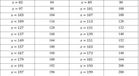
For the curve with equation , : .

Number of Valid Points on the curve over the field of

2 3 3 4

5 4 7 8

11 12 13 20

17 16 19 20

23 24 29 20

31 32 37 36

41 32 43 44

47 48 53 68

59 60 61 52

67 68 71 72

(37)

83 84 89 80

97 80 101 100

103 104 107 108

109 116 113 128

127 128 131 132

137 160 139 140

149 164 151 152

157 180 163 164

167 168 173 148

179 180 181 164

191 192 193 208

197 196 199 200

(38)

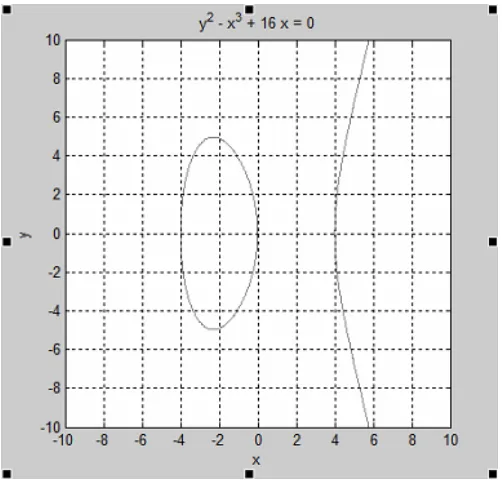
2.2.1.3 Graphical representation of Hyper Elliptic Curve over the real field

, : 2 1 1 2 .

To represent the curve in the graph, the curve has to be drawn over the real number field . Therefore,

, : 2 1 1 2 over

Figure 2.3: Hyper Elliptic Curve over

2.2.1.4 Determining the Cartesian points in a hyper elliptic curve over the real field

When (or more generally, when is a finite field), the elliptic curves over will be a finite set.

Here we take an equation of an elliptic curve with and consider

(39)

Now we want to know what points are on the curve . To do that, we first compute the square table over , which tells us what element in can have a square root. This can be done by using power and mod function in MATLAB.

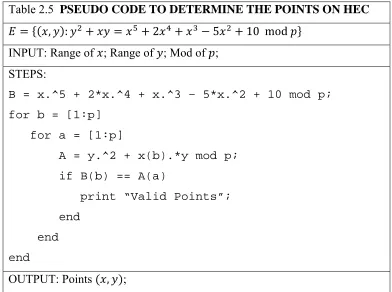
Table 2.5 PSEUDO CODE TO DETERMINE THE POINTS ON HEC

, : 2 5 10 mod

INPUT: Range of ; Range of ; Mod of ; STEPS:

B = x.^5 + 2*x.^4 + x.^3 – 5*x.^2 + 10 mod p;

for b = [1:p]

for a = [1:p]

A = y.^2 + x(b).*y mod p;

if B(b) == A(a)

print “Valid Points”;

end

OUTPUT: Points , ;

In this way we have all the valid points of the curve:

, : 2 5 10 11 ∪

1,4 , 1,6 , 4,2 , 4,5 , 5,7 , 5,10 , 8,0 , 8.3 , 9,5 , 9,8 ,

For the curve with the equation , : 2 5 10 11 has 11

(40)

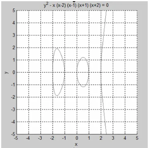
2.2.1.5 Comparing the curves: Elliptic Curves and Hyper Elliptic Curve

Elliptic curve: , : 16 over

Hyper Elliptic curve: , : 2 1 1 2 over

Figure 2.4: Elliptic curve Figure 2.5: Hyper Elliptic curve

By comparing the table 1 and 2, the figure 5 and 6. Hyper elliptic curves to have more number of valid points compare to Elliptic curve. For the field , the curve has 196 valid points, whereas for the

field , , the curve has 206 valid points. Approximate we can comment that have more 10

valid points to . Figure 5 represents an elliptic curve of genus – 1. Genus in plain English means number of loops or holes. Figure 6 represents a hyperelliptic curve. Hyperelliptic curve is also a type elliptic curve with genus – 2, a curve with two holes or two loops.

2.2.1.6 Finding the points on the Hyper Elliptic Curve over large prime field

Let’s take a hyperelliptic curve over a field. The curve : 1184 1846 956 560

over , 2003.

(41)

Here are some of the valid points on the curve: (4,1712), (8,168), (257,1895), (258,783), (1000,1529), (1002,519), (1502,1293), (1505,388), (1999,1232), (2000,818).

2.2.2 Polynomial and Rational Function

Definition 5 (Coordinate Ring, Quotient Ring and Polynomial Function)

If be the ideal of , which is generated by the polynomial , that is

. The quotient ring of , / is also called the coordinate ring of over , denoted by . Elements in the is also called the polynomial functions of over .

It is easy to check that every polynomial, let it be , ∈ , can be uniquely represented in the

form of

,

where the polynomial , ∈ .

Definition 6 (Function Field, Rational Functions)

The function field of over is the field of all fractions of polynomial functions in . An

element of is called a rational function on . A polynomial function is also a rational function. We

have to make a note that is a subring of .

Definition 7 (Degree of a Polynomial Function)

Let , be a polynomial and also a non – zero one in . The degree of the

polynomial is defined to be

(42)

Properties 8 (Degree of a Polynomial Function)

Let , ∈ .

1. deg

2. deg deg deg

3. deg deg ̅

2.2.3 Zeroes and Poles

Definition 12 (Zeros and Poles)

Let ∈ and ∈ . If 0, then is a zero at . If is not defined at , then has a pole at

. Where we write it as ∞.

Definition 13 (Special Point, Zeros)

Let , be a point on the curve C. Let us suppose that the polynomial function ,

∈ has a zero at and is not a root of both and . The ̅ 0 iff is a special

point.

Definition 14 (Ordinary Point, Zeros and Poles)

Let , be an ordinary point on the curve , and , ∈ . Assuming that

0 and is not a root of both of the polynomials and . Then can be written in the form

of , where is the highest power of which divides , and ∈ does not have

(43)

Definition 15 (Special Point, Zeros and Pole)

Let , be a special point on the curve . Then can be written in the form .

(44)

Chapter 3 Hyper Elliptic Curve Cryptography

To realize secure communication over the unsafe internet, cyber security techniques are indispensable such as privacy and authentication. Among these techniques, public key cryptography is an essential in our daily life. This cyber – security technology supports one of the fundamental aspect, like electronic payment infrastructure.

(45)

3.1 Elliptic and Hyper Elliptic Curve Group Law

3.1.1 Arithmetic of Elliptic Curve

Definition 1 (Properties – Elliptic Curve)

An elliptic curve over the field , denoted by / where 3, is given by the Weierstrass

equation.

:

Where the coefficients , , , , ∈ and for the each point , on the curves, the coordinate

, ∈ together with an imaginary point . All the points on the curve must also satisfy the partial

derivatives 2 and 3 2 equals to zero at the same time.

The partial derivative conditions says whether the elliptic curve is non-singular or singular. A point on a curve is called singular if both of the partial derivatives equals to zero.

Definition 2 (Discriminant – Elliptic Curve) [34]

Smoothness of the curves can also be figured out by finding the discriminant of the curve. Let expressions.

4 2 4

4

Let be a curve defined over and let , , and . The discriminant of the curve denoted by ∆

(46)

∆ 8 27 9

3.1.1.1 Group Operations on Elliptic Curve

Definition 3 (Point Addition – Elliptic Curve)

Point Addition P + Q. Denoting the group operation with the symbol " ". “Addition” means that given

two points and their coordinates lies in the curve , say , and , . In this this case

we computer and . A tangent is drawn through the points and and obtain a third

point of intersection. The point of intersection is reflected on the axis to obtain the point on the curve. The figure 1 below shows the point addition on an elliptic curve over .

It is important to define sum of the two points with the same coordinate such as , and , .

In such case it is important to find a neutral element of the group. A further point called the point at infinity or . It can be understood that a point lying far out on the axis such that the line

which is parallel to the axis and passed through the point or . This point at the infinity is called the neutral point or element of the group. Therefore we can conclude that the line passing through ,

and , also passes through or .

(47)

, , , i.e.. ,

Definition 4 (Point Doubling – Elliptic Curve)

Point Doubling P + P. Given two points and their coordinates lies in the curve , say , and

, . In this this case we computer and . Making 2 . A tangent

is drawn through the point and obtain a second point of intersection. The point of intersection is reflected on the axis to obtain the point on the curve. The figure 2 below shows the point addition on an elliptic curve over .

3.1.1.2 Point Addition and Doubling in Elliptic Curve

Point Addition

The simplest form of an elliptic curve is given by the equation

(48)

Let , , , and , . , let the straight line passing through the point

and be: , where, is the gradient of the line and is the – intercept.

The gradient of the line: . The – intercept: at – axis, 0, Therefore,

A point , lies in the elliptic curve if and only if: ,

, , 2

.

Let L.H.S ≡ R.H.S ( )

Or,

Substituting into , .

≡ , , : .

Reflecting the co-ordinate on the – axis. Therefore, ≡ , ,

. Therefore, . .

where, ; if

Point Doubling

The simplest form of an elliptic curve is given by the equation

(49)

Let the line tangent to the curve at be: where, is the gradient of the line tangent and is

the – intercept. The gradient of the line: . The – intercept: at – axis, 0. Or,

, , . Therefore,

A point , lies in the elliptic curve if and only if: ,

, , 2

2 2

Let L.H.S ≡ R.H.S ( ): 2 , 2

Substituting into , . ≡ , .

: 2 ,

Reflecting the co-ordinate on the – axis. Therefore, ≡ , 2 , .

Therefore, 2 , . Where,

3.1.2 Arithmetic of Hyper Elliptic Curves

3.1.2.1 Group Operations on Hyper Elliptic Curves

In elliptic curves we can take the points on the curve with the point of infinity to form a group. However for the hyper elliptic curves, if we take the points on the curve and with the points of infinity cannot no longer form a group. To form a group with respect to the points of hyper elliptic curve, we need to take

sum of points as group elements and then we can perform addition like ⨁

(50)

If we start to form group by this expression ⨁ , then we would end up with an infinite group and larger and larger representation of the group elements. In this case we use the quotient group of the group based on the all sum of points that lie on the curve.

Below we give a graphical representation of a hyper elliptic curve for a genus 2 over the finite field

given by the equation . This equation of the curve must fulfill the five conditions

before we can perform group operation.

Hyper elliptic curve of genus over the finite field in the set of points in such that:

C: .

Conditions:

1. , ∈ .

2. → monic, and deg 2 1 is odd.

3. deg , if 2; 0 if 2.

4. The curve HEC doesn’t have any singular point over .

5. 2: , where is monic, odd – degree and square free.

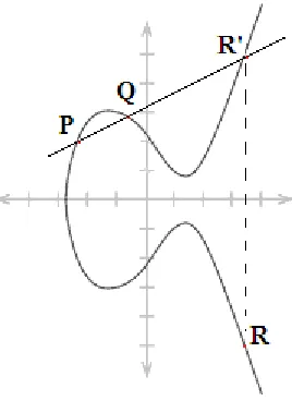
Figure 3.3: Group operation on the HEC of genus 2 over , ,

deg 5 and is monic for ⨁ .

(51)

As discussed before that the chord and tangent method in the elliptic curve cannot be used. The curve which intersects with the hyper elliptic curve of genus 2 shown above is called Jacobian variety curve. The Jacobian curve intersects in 5 points instead of 3 points unlike chord and tangent method in elliptic curve. In order to build a group we take the quotient group; which is the sum of the intersecting points of the Jacobian variety curve with the hyper elliptic curve by the subset of the points which lie on the HEC.

The six points , , , and on the HE curve adds upto zero in the quotient group. The point

, and , lie on the curve. Similarly, ⨁ 0. The points and

are the reflection of the points and on the HE curve respectively. And the resulting group

operation ⨁ .

3.1.2.2 Divisor and Divisor Class Group. [37], [38]

Definition 5 (Divisor)

The rational points of a hyper elliptic curve do not form a group, unlike the points on an elliptic curve. The group which provides by the hyper elliptic curve for cryptography is a subgroup of the random group generated by the set of points on the curve. If the curve is the hyper elliptic curve of genus over the finite field . The elements of is known as divisors.

∑ , ∈ and ∈

Definition 6 (Group of divisors)

For the hyper elliptic curve of genus over the finite field given by an equation of the form C:

. The group of divisors of the curve of degree 0 is given by

∑ ∈ | ∈ , 0, for most of the points on the curve ∈ .

(52)

into the divisor class group. Since in this thesis we are considering the hyper elliptic curve of deg

odd. Therefore, there is only a single point at the infinity. However, if we were working on the hyper elliptic curve of def even, then there would have been two point of infinity. To visualize this we can imagine a point far on the axis such that any line which is parallel to it passes through the point

.

Definition 7 (Divisor Class Group)

The divisor class group of is the quotient group of the group of divisors . In the divisor class group, each divisor class can be represented by

∑ , ∈ including the point , .

By using the definition above. The individual divisor class can be represented for implementation purpose. The divisor class group of is isomorphic to the finite field of of the Jacobian of the hyper

elliptic curve .

3.1.2.3 Jacobian variety of Hyper Elliptic Curve

Definition 8 (Jacobian) [39], [40]

The Jacobian of the curve is defined by the quotient group:

/

Hence, , ∈ are equivalent if ∈ . In every equivalence class there’s only one divisor

, called the reduced divisor:

(53)

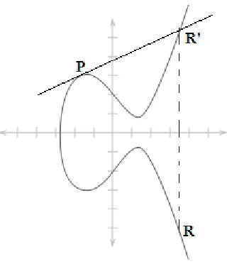
Jacobian variety curve in a specific curve based on the Jacobian . In simple form, the intersection points between the Jacobian variety curve with the hyper elliptic curve forms a group including the point at the infinity . Where the sum of the all the intersecting point sums up to zero. The figure below is the graphical representation of the Jacobian variety and the hyper elliptic curve of genus 2.

Figure 3.4: Hyper Elliptic Curve of genus 2 and Jacobian Variety Curve.

Since the intersection points between the Jacobian variety curve with the hyper elliptic curve sums up to zero. Therefore:

0.

.

The Cartesian or affine space points and could be transformed to individual divisor class group based on Mumford Representation, which is to be discussed in a separate section.

The divisor class, , ∪ , . Similarly , ∪

, and , ∪ , . The expression and are the

(54)

3.2 Point Representation - Divisor

The definition of the divisor group is the simplest form of representation. However, we can represent the divisors just as the sum of points with the order of the points .

∈

The disadvantage of representing the divisor is that we cannot use this for computational purposes. To represent the points in the form of divisor the best option in the Mumford Representation.

3.2.1 Mumford Representation [35], [36]

Mumford representation is the clearest representation of the Cartesian points into polynomial divisor form.

The divisor can be represented with two polynomial as and . Let be the individual reduced

divisor of the divisor class group of .

One fundamental reason for using the Mumford Representation is that this representation can be used for computing purpose. Let consider a hyper elliptic curve of genus , where the curve is

represented as:

where the polynomial expressions and ∈ the polynomial field , the deg 2 1

and the deg . As discussed before that the divisor class over the field can be represented by a

pair of polynomials and , where this polynomials , ∈ .

Although the polynomials and belongs to the polynomial field of . However this

(55)

Conditions:

1. must a monic polynomial.

2.deg deg .

3. | .

The polynomial expression of of the divisor class is represented by:

Where the divisor class is represented as shown below.

The point , and the points , lies on the curve. If the points on the curve occurs

number of times then

0

Where and 0 1. In the hyper elliptic curve of genus 2, each divisor class can be

represented by the 4 coefficients , , , of the polynomials and . The divisor class

represented by the polynomials and as , .

However, the divisor class group of is the quotient group of the group of divisors . So the

identify or neutral elements, in this case its neutral divisor class of the group is represented as 1,0 .

(56)

3.2.2 Mumford Representation – An example

In this example we consider the hyper elliptic curve : 3 2 3 of genus 2 over

the field . The Cartesian points 3,0 , 1,2 , 4,1 and 3,0 . The divisor class

group of is the quotient group of the group of divisors . Each divisor class can be

represented by including the point , .

Taking the points 3,0 , 1,2 , where 3 and 1. The polynomial expression of

of the divisor class is represented by:

Therefore, ∏ and ∏ 3 1

4 3 3 over the polynomial field of . The polynomial 3 ∈

.

The condition for finding the polynomial expression must satisfy the second and the third condition

(2). deg deg and (3). | respectively. Since the degree of

is less than the degree of , the polynomial expression of would appear as

.

The number of combinations of , where ∈ 0.1.2.3.4 . The possible combinations we can

get for , are:

0,0 1,0 2,0 3,0 4,0

(57)

0,3 1,3 2,3 3,3 4,3 0,4 1,4 2,4 3,4 4,4

Any of the combination of , will satisfy the third condition | . In this

case the combination , 4,3 satisfies the condition mentioned above.

Therefore, the Mumford representation of the point 3,0 and 1,2 on the hyper elliptic curve

: 3 2 3 of genus 2 over the field is:

3,4 3

Similarly, the Cartesian points 4,1 and 3,0 can be represented in Mumford form.

(58)

Chapter 4 An Overview of Hyper Elliptic Curve

Computation Method

In this chapter we will discuss Hyper Elliptic Curve Computation Methods for performing group operations, such as addition and doubling of the divisor classes of hyper elliptic curves discussed in the previous chapter. The purpose of this chapter is to discuss in detail on how we perform the group operations of the divisor class group obtained from the Jacobians of the hyper elliptic curves. The intersecting points of the Jacobian variety curve with the hyper elliptic curves seems to form a group [19].

However, the arithmetic operations of the divisor classes in the hyper elliptic curve was usually performed by using Cantor Algorithm. Cantor algorithm has been optimized by Harley, and the first to obtain subexpression and explicit formulas for the hyper elliptic curves of genus 2 and later in was extended by Lange and others.

Here we concentrate on the hyper elliptic curves of genus 2, 3 and 4 and provide an efficient explicit formulae for performing the arithmetic operations such as addition and doubling in HEC. The first explicit formula for genus 4 curves in to be found in this chapter.

4.1 Cantor Algorithm

(59)

4.1.1 Composition and Reduction Stage

Let consider a hyper elliptic curve of genus , where the curve is represented as [1]:

where the polynomial expressions and ∈ the polynomial field , the deg 2 1

and the deg . As discussed before that the divisor class over the field can be represented by a

pair of polynomials and , where this polynomials , ∈ .

Here the polynomials and of the divisor class are the representation of the intersection points between the Jacobian variety curve and the hyper elliptic curve in Mumford form. The divisor class

, .

In the composition section of the Cantor Algorithm, the algorithm takes the polynomial expression

and ∈ . The Mumford representation of the points , and , in the divisor class:

, & , . Here the polynomials , , , ∈ . The

algorithm below performs the calculation for: .

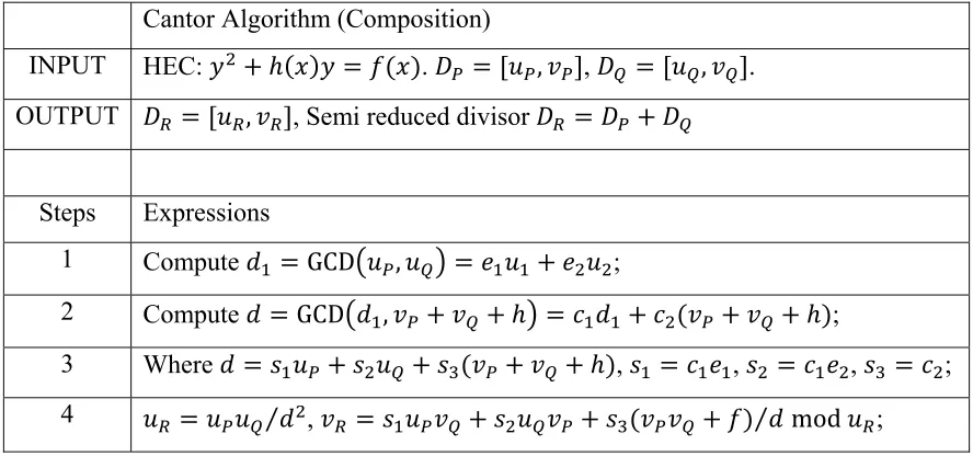
Cantor Algorithm (Composition)

INPUT HEC: . , , , .

OUTPUT , , Semi reduced divisor

Steps Expressions

1 Compute GCD , ;

2 Compute GCD , ;

3 Where , , , ;

4 _⁄ _, _⁄ _mod _;

(60)

In the step 1, is the resultant polynomial expression found by calculating the greatest

common divisor GCD of the two polynomials and . In the step 2,

resultant polynomial expression found by calculating the GCD of the two polynomials and the sum of

the polynomials . The expression in the step 2 can be represented as , and . The step

4 calculates the expression for and reduced expression of mod .

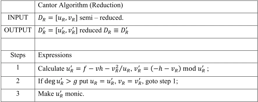
Cantor Algorithm (Reduction)

INPUT , semi – reduced.

OUTPUT , reduced ≡

Steps Expressions

1 _Calculate ⁄ , mod ;

2 If deg put , , goto step 1;

3 Make monic.

Table 4.2: Cantor Algorithm (Reduction)

The divisor is known as semi reduced as calculated in the composition section. That means

it is possible for further reduction. The second part of the Cantor Algorithm (Reduction) can be used to further reduce the polynomials expression of and . The result of the composition section can be used to perform further calculation. However it is better in practice to reduce the two polynomial expressions. In the section below, we have presented an example which will clear the mathematical steps in the Cantor Algorithm.

4.1.2 Cantor Algorithm – An example

In this example we consider the hyper elliptic curve : 3 7 2 of genus 2 over the

field . The divisor , 7 10, 9 and , 10, 7 9 .

Here the polynomial expression 3 7 2, , , and ∈ . The step

(61)

compute GCD , . So we can rewrite this expression as GCD 7

10, 10 .

Here, the GCD is calculated by using Extended Euclidean Algorithm as shown below:

7 10 10 GCD 7 10, 10

1 0 7 10

0 1 10 1

1 1 7 8

3 8 1 10 4

0

Therefore, 3 7 10 8 1 10 . In step 2, we need to

compute GCD , . So we can rewrite this expression as

GCD 10,8 10 . Here, the GCD is calculated by using Extended Euclidean Algorithm as shown below:

8 7 10 gcd 10, 8 7

1 0 8 7

0 1 10 3 4

0

Therefore, 1 10 0 8 7 . In the step 3, we need to represent the

result of step 3 as . Where we need to calculate 1

3 3 , 1 8 1 8 1 and 0. In the step 4, ⁄

(62)

⁄ mod 4 7 5. So, the semi reduced divisor

7 9 4 1, 4 7 5 . In the step 1 of the Cantor Algorithm (Reduction), we

calculate ⁄ 10 and mod 6. Working on the step 2 and

3 of the algorithm the reduced divisor . 10,6 in Mumford Representation.

4.1.3 Advantages and Disadvantages of using Cantor Algorithm

Cantor Algorithm was the first solid algorithm to perform the computations in the Jacobian groups of hyper elliptic curves over the fields of odd characteristics. The biggest advantage of the Cantor Algorithm is that we can apply this algorithm for any hyper elliptic curve of any genus over any field. Although the Cantor Algorithm is very computationally intensive, it can perform divisor class operations on hyper elliptic curves of any properties. The disadvantage lies in its computationally intensiveness. In the step 1 and 2 of its composition section, both of the steps uses Extended Euclidean Algorithm to calculate the GCD, which is computationally very intensive. Calculating GCD requires polynomial multiplication and especially polynomial inverses, which is computationally intensive. Other steps also requires polynomial multiplication and inverses. The Cantor Algorithm only offers the addition operation. For the scalar multiplication or doubling, the algorithm needs to be repeated. The table below shows the complexity of the Cantor Algorithm for genus 4 hyper elliptic curve over the field .

Algorithm Inversion Addition Operation

(I) Multiplication

(M)

Squaring (S)

Cantor [23] 6 386 M/S

(63)

4.2 Subexpression Algorithm

Similarly like the Cantor Algorithm, Subexpression Algorithm [11] considers a hyper elliptic curve of

genus , where the curve is represented as: where the polynomial expressions

and ∈ the polynomial field , the deg 2 1 and the deg . As discussed before

that the divisor class over the field can be represented by a pair of polynomials and , where

this polynomials , ∈ . The divisor class , . The algorithm below performs

the calculation for: .

Subexpression Algorithm [24]

INPUT Genus = 2, HEC: . , , , .

, ; ,

;

OUTPUT , , , ;

Steps Expressions

1 ⁄ ;

2 ⁄ mod ;

3 ∙ ;

4 ⁄ ;

5 made monic;

6 _mod _;

(64)

The algorithm above performs addition operation between the two divisor classes. Similar algorithm

below performs the doubling operation for: 2 .

Subexpression Algorithm [24]

INPUT Genus = 2, HEC: . , , ,

;

OUTPUT 2 , ;

Steps Expressions Steps Expression

1 ⁄ 4 2 ⁄

2 ⁄ 2 mod 5 made monic

3 ⋅ 6 ≡ mod

Table 4.5: Subexpression Algorithm (Doubling)

4.2.1 Subexpression Algorithm – An example

Using the same example used in the section of Cantor Algorithm – An example. Considering the hyper

elliptic curve : 3 7 2 of genus 2 over the field . The divisor ,

7 10, 9 and , 10, 7 9 . Here the polynomial expression

3 7 2, , , and ∈ .

In the step 1, we calculate the expression, ⁄ ;

3 7 2 7 9 ⋅ 0 7 9 ⁄ 10

Therefore, 4 2.

(65)

9 7 9 ⁄ 10 mod 7 10

Therefore, 4.

In the step 3,4 and 5. We calculate the expression, ∙ 4 7, the expression

⁄ 10 and the expression made monic 10.

Finally in the step 6, we calculate the expression, mod 6.

10,6 in Mumford Representation.

4.2.2 Advantages and Disadvantages of using Subexpression Algorithm

The algorithms takes the polynomial representation of the divisor class of Cartesian points in Mumford

Representation and also the polynomial expression of and . The biggest advantage of the

Subexpression Algorithm is that, unlike the Cantor Algorithm which uses Extended Euclidean Algorithm twice to calculate GCD. In this algorithm, we don’t have to compute GCD, which saves a lot of computationally intensive calculations such as polynomial inverses and multiplication.

The disadvantage lies in its computationally intensiveness. All the steps requires polynomial multiplication and especially polynomial inverses, which is computationally intensive. Unlike Cantor Algorithm, which can be applied to any hyper elliptic curve of any number of genus’s, this algorithm is limited to the hyper elliptic curve of genus 2.

4.3 Explicit Formulae Algorithm

(66)

explicit formula for genus 2 and for odd characteristics was made by Harley [11] and later was derived to have an explicit formula for even characteristics by Lange [9].

Matsuo, Chao and Tsujii [13] has already presented an explicit formulae for addition and doubling operation. To reduce the number of inversions to 1, Miyamoto, Doi, Matsuo, Chao and Tsujii [14] and the work by Takahashi [15] had obtained by using Montgomery trick.

4.3.1 Advantages and Disadvantages on Explicit Formulae Algorithm

Unlike Cantor Algorithm and Subexpression, which uses computationally intensive polynomial multiplication and inverses. Explicit formula only takes the co-efficient of the input polynomial and perform integer multiplication, inverses and squaring.

The only disadvantage of Explicit Formulae over the Cantor Algorithm is we need to derive separate explicit formula for the hyper elliptic curve of genus 2, 3, 4 and further. Unlike Cantor Algorithm, where we can use the same algorithm for performing group operation such as addition and doubling. Explicit formula has separate algorithms for addition and doubling operation.

(67)

Chapter 5 Proposed Efficient Computation for Hyper

Elliptic Curve Cryptography

In this chapter, we will discuss the proposed efficient explicit formulae algorithm for group operation. Also the theorems and proposition used to build an efficient explicit formulae algorithm. Separate explicit formula algorithm for addition and doubling for specific hyper elliptic curve with different number of genus.

5.1 Explicit Formulae Algorithm for Hyper Elliptic Curve for genus 2

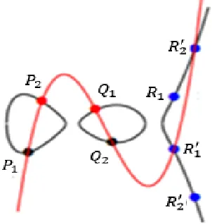
As discuss before that the group law operations in the Jacobian. The intersecting points of the Jacobian variety curve with the hyper elliptic curve form a group. In the section 3.1.2.3 of Jacobian variety of Hyper Elliptic Curve, we have mentioned that that Jacobian variety curve is a specific curve and its intersecting points with the hyper elliptic curve for a group including the point at the infinity . Where the intersecting points sums to zero. The figure below is the graphical representation of the Jacobian variety curve and the hyper elliptic curve of genus 2.

(68)

Since the intersection points between the Jacobian variety curve with the hyper elliptic curve sums up to zero. Therefore:

0.

.

The Cartesian or affine space points and could be transformed to individual divisor class group based on Mumford Representation, which is to be discussed in a separate section.

In the section 3.2.2 Mumford Representation – An example, we have shown how we can convert the Cartesian points on the curve into polynomial expression based on Mumford. By applying Mumford Representation, we can convert all the Cartesian points into divisors, after the conversion we can obtain

the equation for the Jacobian Variety curve. Here we denote the Jacobian curve as .

5.1.1 Generating General Addition Explicit Formula for HEC of genus 2

Let’s consider a general Hyper Elliptic Curve of genus 2 over the finite field :

HEC:

The intersecting coordinates , and , would be converted to polynomial

expression using Mumford.

The divisor class group, for the point , , for the point , and for the point , as

shown below:

2 ,

(69)

2 ,

From the figure 1 above we can assert the polynomial expression of to be

. The Jacobian curve is a cubic function since we can see in the graph that the function has two extreme points and intersecting with the hyper elliptic curve with six Cartesian points.

At the intersecting points the y-coordinates are same. Therefore we can write, at the intersection points

or ≡ 0 since we have to perform polynomial reduction.

For the intersecting points and , we can write it in the form of ≡ 0 .

≡ 0 mod

Or, ≡ mod

By reducing the L.H.S with the polynomial expression and comparing with the R.H.S,

we get four simultaneous equations.

≡ EQN 1

≡ EQN 2

≡ EQN 3

≡ EQN 4

Subtracting the EQN 1 from EQN 3, we get: