University of Windsor University of Windsor
Scholarship at UWindsor
Scholarship at UWindsor
Electronic Theses and Dissertations Theses, Dissertations, and Major Papers
2012
Fast Modular Reduction for Large-Integer Multiplication
Fast Modular Reduction for Large-Integer Multiplication
Suhas Sreehari University of Windsor
Follow this and additional works at: https://scholar.uwindsor.ca/etd
Recommended Citation Recommended Citation
Sreehari, Suhas, "Fast Modular Reduction for Large-Integer Multiplication" (2012). Electronic Theses and Dissertations. 5360.
https://scholar.uwindsor.ca/etd/5360
Fast Modular Reduction for Large-Integer Multiplication
by
Suhas Sreehari
A Thesis
Submitted to the Faculty of Graduate Studies through Electrical and Computer Engineering in Partial Fulfillment of the Requirements for the Degree of Master of Applied Science at the
University of Windsor
Windsor, Ontario, Canada
2012
Fast Modular Reduction for Large-Integer Multiplication
by
Suhas Sreehari
APPROVED BY:
______________________________________________ Dr. A. Reza Riahi
Department of Mechanical, Automotive and Materials Engineering
______________________________________________ Dr. Mohammed A.S. Khalid
Department of Electrical and Computer Engineering
______________________________________________ Dr. Majid Ahmadi, Co-Advisor
Department of Electrical and Computer Engineering
______________________________________________ Dr. Huapeng Wu, Co-Advisor
Department of Electrical and Computer Engineering
______________________________________________ Dr. Govinda Raju, Chair of Defense
Department of Electrical and Computer Engineering
DECLARATION OF ORIGINALITY
I hereby certify that I am the sole author of this thesis and that no part of this thesis has
been published or submitted for publication.
I certify that, to the best of my knowledge, my thesis does not infringe upon anyone’s
copyright nor violate any proprietary rights and that any ideas, techniques, quotations, or
any other material from the work of other people included in my thesis, published or
otherwise, are fully acknowledged in accordance with the standard referencing practices.
Furthermore, to the extent that I have included copyrighted material that surpasses the
bounds of fair dealing within the meaning of the Canada Copyright Act, I certify that I
have obtained a written permission from the copyright owner(s) to include such
material(s) in my thesis and have included copies of such copyright clearances to my
appendix.
I declare that this is a true copy of my thesis, including any final revisions, as approved
by my thesis committee and the Graduate Studies office, and that this thesis has not been
ABSTRACT
The work contained in this thesis is a representation of the successful attempt to speed-up
the modular reduction as an independent step of modular multiplication, which is the
central operation in public-key cryptosystems. Based on the properties of Mersenne and
Quasi-Mersenne primes, four distinct sets of moduli have been described, which are
responsible for converting the single-precision multiplication prevalent in many of
today's techniques into an addition operation and a few simple shift operations. A novel
algorithm has been proposed for modular folding. With the backing of the special moduli
sets, the proposed algorithm is shown to outperform (speed-wise) the Modified Barrett
algorithm by 80% for operands of length 700 bits, the least speed-up being around 70%
ACKNOWLEDGEMENTS
“No stream or gas drives anything until it is confined. No Niagara is ever turned into light
and power until it is tunneled. No effort ever grows great until it is focused, channeled,
dedicated and disciplined.” This is what one of my undergraduate professors always says.
I realized that first hand during the two years I spent at the University of Windsor. I still
remember how I was at the beginning of my MASc program. I was excited, but clueless.
I had studied several courses during my undergraduate years too, but it was the first time
I was about to conduct research. It meant I had to find out something, do something,
however tiny – that no one else had done before. Not just that, whatever I do has to be
useful. That is where my supervisors came into picture.
Dr. Huapeng Wu (my supervisor) taught me a lot about feasibility. He showed me the
importance of always staying on top of literature, and made sure my research did not
become obsolete. Dr. Majid Ahmadi (my co-supervisor) spent a lot of time motivating
me, and always encouraged me to try new things. Without the constant support and
supervision of these two professors, I would not have put together the work contained in
this thesis. I also would like to thank Dr. Reza Riahi (my external program reader) and
Dr. Mohammed Khalid (my department reader) for their time and constructive
Payal Khanwani deserves my heartfelt gratitude for all her support and love. Ms. Andria
Ballo (ECE graduate secretary) and Ms. Rachelle Marchand (ECE undergraduate
secretary) have been thoroughly patient (I have run to them all the time for every small
thing) and have indirectly helped me graduate with success.
Finally, I would like to mention the continuous support from my family, and their faith in
TABLE OF CONTENTS
DECLARATION OF ORIGINALITY iii
ABSTRACT iv
DEDICATION v
ACKNOWLEDGEMENTS vi
LIST OF FIGURES x
Chapter I: Introduction 1
1.1 Defining Large 1
1.2 Motivation 2
1.3 The big picture 4
1.4 Organization of the thesis 5
Chapter II: Preliminaries 7
2.1 Recapitulating abstract algebra 7
2.2 Finite fields and arithmetic 14
2.3 Prime numbers 16
2.4 Public-key cryptography 18
2.5 RSA cryptography 21
Chapter III: Historical overview and technical survey 25
3.1 Large-integer multiplication 25
3.2 Modular multiplication/reduction techniques 38
Chapter IV: Proposed method and results 50
4.2 Results 59
Chapter V: Conclusion and future work 63
5.1 A summarized view of the thesis 63
5.2 Scope for future work 66
REFERENCES 67
LIST OF FIGURES
Figure 1: The Big Picture 4
Figure 2: A simplified illustration of public-key cryptography (for data security) 21
Figure 3: A brief timeline of the some important works pertaining to modular
reduction geared towards multiplication 40
Figure 4: Time delay comparison 62
Figure 5: Time delay comparison – smoothed graph 62
CHAPTER I
INTRODUCTION
“Lots of people working in cryptography have no deep concern with real application
issues. They are trying to discover things clever enough to write papers about.”
- Whitfield Diffie (of the Diffie-Hellman Key Exchange fame)
I hope and believe my work presented in this thesis does not put me with those “lots of
people”.
1.1Defining “large”
Arithmetic operations are the often thought of to be the most understood concepts. While
this seems to be true for smaller bit-lengths, the situation gets trickier in that the
school-book method that works so well in implementing smaller operand-arithmetic suddenly
seems slower and cumbersome in implementing the arithmetic for large operands. Now,
“large” is a subjective qualifier, and it is hard to put a number on it in generic terms.
What is large for one application could be not-so-large or even small for another. So it is
important that we outline the application we are targeting the development of the current
arithmetic towards. The operation in question throughout this thesis is the
multiplier-based modular reduction of a large integer. Application-wise, this would be a typical step
in modular exponentiation – which is routinely carried out in RSA cryptography. In this
the lower end and up to a 200-bit tail at the upper end making the extended range much
wider, from 150 to 700 bits in length. However, in this thesis, when not explicitly
mentioned, a safe assumption is that a large integer is around 500 bits long, on an
average.
Now that there is some clarity as to what constitutes a large integer for our purposes, let
us see where the problem tackled in this thesis fits (in the big picture) and more
importantly, what the problem I have solved is.
1.2Motivation
Very simply put, the problem this thesis sets out to solve, and subsequently solved, is to
speed up the computation of the product of two large integers modulo a prime modulus
half the bit-length of the product. Now, there exist many solutions (some of which are
neat and elegant) to multiply two large integers – whatever way, be it bit-serially, or
word-serially, or in parallel, depending on the time, area, and power considerations and
based on the available restrictions and resources.
Then we have algorithms which multiply and modulo-reduce integers alternatively,
taking small chunks of the operands, in a sliding windowed fashion. This method is
generally word-serial.
There are very famous algorithms to reduce large integers. It came to my notice early on
compared to amount of time and effort spent by the research community on improving
multiplier designs.
After recognizing these three broad categories, it was decided to investigate the merits
and demerits of all three approaches before adopting one for this thesis work. Not to put
too fine a point upon it, let us see the high-level factors which helped in deciding which
stream to choose.
Based on [30], the word-serial multiply-reduce alternation scheme was ruled out because
there is almost no speed gain in this method compared to first multiplying the large
integers, and following it up with reduction. However, in separating multiplication and
reduction, the freedom gained in terms of using algorithms independently of each other
(for multiplication and reduction) – as long as there is basic I/O compatibility – is
enormous. This shines the spotlight on three possibilities – (i) working on the multiplier
unit, or (ii) working on the reduction unit, or (iii) working on both. Time restrictions on
master’s degree took care of eliminating the third option. As for working on the
multiplier, there exist many innovative algorithms and seems to be the general focus of
researchers. The scope for improvement is bigger in the reduction unit camp, and it was
felt that this research area is somewhat neglected, if not abandoned. These realizations
provided enough clarity and motivation to work mainly on the reduction unit, while
adopting the best multiplier unit to go with it, to build a complete modular multiplier
1.3The big picture
To remain sufficiently motivated and clear about the problem (and the corresponding
solution proposed in this thesis), it is essential we resort to the big picture.
Fig. 1: The Big Picture
As we can see in Fig. 1, Modular Reduction forms an integral part of Modular
Multiplication, which in turn is an important step in carrying out Modular Exponentiation
operations. Modular Exponentiation operations are the backbone of any RSA
cryptosystem implementation, but are very expensive in terms of hardware complexity.
Therefore, speeding up Modular Reduction at the lowest level has far reaching
1.4Organization of the thesis
The thesis is organized in such a way to retain maximum clarity and focus on the problem
of central importance. As we have already seen, Chapter 1 (the introductory chapter) has
been kept relatively succinct to the point of highlighting the motivation and academic
justification for choosing the problem this thesis has indeed succeeded in bringing about
the desired solution for.
Chapter 2 is solely dedicated to rapidly bring any novice reader up to the technical
comfort, that is required to not only grasp the implications of the work and results
presented in this thesis, but also to fully appreciate and add to the existing richness by
way of constructive critiques and/or augmenting the work as suggested in the last chapter,
under the section which delineates possibilities for future work. To achieve this clear-cut
objective, crisp explanations of certain well-known and required mathematical models,
slowly built up from more accessible mathematical foundations, have been included. As a
result, any scholar in this area might find it tempting (and justifiably so) to skip this
chapter.
Chapter 3 makes best use of the knowledge built up in Chapter 2, by introducing the
state-of-the-art work in this area, in a phased manner. Now, what is meant by a phased
overview of the evolution of this research area, and is seamlessly merged into the most
modern work, in a blurred boundary fashion.
Chapter 4 is a portrayal of the original work and contribution of this thesis to extending
the envelope of the state-of-the-art technique in speeding up Modular Reduction, in a
backwards compatibility mode with the most widely used classic multiplication
algorithms. The theoretical formulation of the solution is immediately backed by FPGA
implementation results of the proposed algorithm, and the chapter concludes with the
concurrence of the expected result (from the theoretical side) and the achieved results
(from the implementation side), thus validating the claims made in this thesis.
Chapter 5 is a rather short, but tight stitch-up of the myriad ideas scattered throughout the
thesis, so as to form one self-contained block which encompasses the problem, the
deficiencies of existing solutions, my proposed solution, why my solution works, and
CHAPTER II
PRELIMINARIES
In this portion of the thesis, a narrow down strategy is adopted to get to the problem
definition. Actually, it is only in the next section that the problem would be defined in
explicit terms, but the role of the current section is to provide the reader with ample
mathematical and conceptual background in order to better understand the future sections
lined up.
To that end, the basics of abstract algebra would be covered, brushing along group
theory, and diving into finite fields and their arithmetic. Once we are done with the
special arithmetic defined within finite fields, the platform would be set for a general
introduction to the working of the public-key cryptographical technique outlined by
Rivest, Shamir, and Adleman, now widely known as “RSA cryptography”.
2.1Recapitulating abstract algebra
The study of algebraic structures like groups, fields, rings, and vector spaces fall into the
purview of “abstract algebra”. The term abstract algebra came into being at the
beginning of the 20th century and it helped distinguish this area from elementary algebra
which deals with the algebraic expressions, their solutions, with real and imaginary
Major themes handled in abstract algebra range from solution of systems of linear
equations, which lead to linear algebra to closed form expressions representing the
solutions of general polynomial equations of higher degree that resulted in discovery of
groups as abstract manifestations of symmetry. Beyond this, arithmetical investigations
of quadratic and higher degree forms and Diophantine equations have been carried out in
this area of mathematics. There are several problems that figure in the grasp of abstract
algebra, but we will stop here as the point of how important and influential this branch of
modern mathematics is, is made well.
Now, we shall begin the exploration from basic set theory, and then move on to groups.
2.1.1Sets
A “set” simply is a collection of well-defined entities/objects, which are connected
together by some common thread – which would serve as the characteristic of the set.
The members of a set are called elements of the set. Basic examples of sets could be,
W = {Violet, Indigo, Blue, Green, Yellow, Orange, Red}, where W is the set of all the
colours in white light.
In a lot of cases, enumeration of the elements of a set is often impractical, and tedious.
Some sets are even infinite, in which case enumeration is not even possible. In all those
situations, stating the rule which governs the set is the best way to describe the set.
Suppose E is an element of set A. Then, it is represented by E ∈ A (read “E belongs to
A”). However, if an element F (which is an element of another set C) is not an element of
set A, then we write F ∉ A (read “F does not belong to A”).
It is possible that one could identify one set as being fully a part of another. In set theory
language, this is the concept of “sub-sets”. If A and B are two sets, and if A is fully
encompassed in B, then we say that A is a subset of B, denoted by A ⊆ B. This means
that all the elements of set A are also elements of set B. Now, if set B has elements that
are not found in set A, A is called a proper subset of B, denoted by A ⊂ B. A very simple
example would be,
A = {2, 3, 5, 7}, where A is the set of prime numbers between 0 and 9.
B = {2, 3, 5, 7, 11, 13, 17}, where B is the set of prime numbers between 0 and 19.
It is fairly easy to see that the elements of A are completely contained in set B, and also
set B has more elements that set A does not. In other words, A ⊂ B.
Further, the number of elements in any set is called the “cardinality” of the set, or simply
the cardinal number. The reader may wish to recall the operations that are usually defined
over sets, such as unions, intersections, Cartesian products, and inversions (generally
It is time to move on to the topic of primary importance in modern algebra – “algebraic
structures”. We come across various types of structures, and let us see what those are.
2.1.2Algebraic structures
An algebraic structure contains multiple sets, closed under certain operations. Groups,
fields, and rings are all structures. Broadly, structures are divided into two kinds – those
whose axioms are identities, and those in which some axioms may not be identities.
Group-like structures belong to the former category, while field-like structures belong to
the latter category. We will touch upon groups and fields later. All the axioms mentioned
hereunder are taken from Peter Cameron’s course notes on algebraic structures [1].
2.1.3Groups
A group is an algebraic structure with just one binary operation, and it satisfies four
axioms:
(G0) (Closure law) For any g,h ∈ G, we have g * h ∈ G.
(G1) (Associative law) For any g,h,k ∈ G, we have (g * h) * k = g * (h * k).
(G2) (Identity law) There is an element e ∈ G with the property that g*e=e*g=g for all g
∈ G. (The element e is called the identity element of G.)
(G3) (Inverse law) For any element g ∈ G, there is an element h ∈ G satisfying g * h = h
Additionally, if the group G satisfies the following law, then it is termed an “Abelian
Group”:
(G4) (Commutative law) For any g,h ∈ G, we have g * h = h * g.
2.1.4 Rings
A ring is defined by two operations: addition (+) and multiplication (.). Sometimes, we
ignore the “.” In the multiplication, and simply concatenate the operands. We define a
ring to be a set R with two binary operations satisfying the following axioms.
Axioms for addition:
(A0) (Closure law) For any a,b ∈ R, we have a+b ∈ R.
(A1) (Associative law) For any a,b,c ∈ R, we have (a+b)+c = a+(b+c).
(A2) (Identity law) There is an element 0 ∈ R with the property that a+0 =
0+a = a for all a ∈ R. (The element 0 is called the identity element of
R.)
(A3) (Inverse law) For any element a ∈ R, there is an element b ∈ R satisfying
a+b = b+a = 0. (This element is −a, and we call it the additive inverse of a.)
(M0) (Closure law) For any a,b ∈ R, we have ab ∈ R.
(M1) (Associative law) For any a,b,c ∈ R, we have (ab)c = a(bc)
Apart from those, we do have a mixed axiom as well:
(D) (Distributive laws) For any a,b,c ∈ R, we have (a+b)c = ac+bc and
c(a+b) = ca+cb.
These are the basic axioms in place. However, there are further multiplicative properties
listed below:
(M2) (Identity law) There is an element 1 ∈ R such that a1 = 1a = a, for all a ∈ R. (The
element 1 is called the identity element of R.)
(M3) (Inverse law) For any a ∈ R, if a=0, then there exists an element b ∈ R such that ab
= ba = 1. (We denote this element b by a−1, and call it the multiplicative inverse of a.)
(M4) (Commutative law) For all a,b ∈ R, we have ab = ba.
A ring which satisfies (M2) is termed a ring with identity; a ring which satisfies (M2) and
(M3) is termed a division ring; and a ring which satisfies (M4) is termed a commutative
ring.
A ring which satisfies all (M2), (M3), and (M4), is called a “field”. A ring can have
2.1.5Fields
In modern algebra, fields are a class of rings. Perhaps the simplest definition of a field is
that it is a commutative ring, the non-zero elements of which form a group under
multiplication. What this immediately means is that a ring has a looser existence than a
field. A field is expected to have more than one element, thus ruling out the trivial
solution that comes from a zero element ring. The specific advantage of a field comes in
the form of division by non-zero elements, which is not allowed in a ring.
A field has a useful feature of being capable as a scalar for a vector space, which is the
standard general context for linear algebra. The theory of field extensions (which
includes Galois theory) involves polynomial roots with coefficients in a field. In modern
mathematics, number theory is greatly benefitted by field theory. There are several other
areas within mathematics depending on fields, rendering the theory of fields extremely
important.
The easiest way to check if a set F is a field is by checking for the following:
1. Closure of F under addition and multiplication:
For any a, b ∈ F, a+b ∈ F and ab ∈ F.
2. Associativity under addition and multiplication:
For any a, b, c ∈ F, we have, a+(b+c) = (a+b)+c and a(bc) = (ab)c.
3. Commutativity under addition and multiplication:
For any a, b ∈ F, we have, a+b = b+a and ab = ba.
There exists an element, 0 ∈ F, such that for any a ∈ F, a+0 = a. “0” is called the additive
identity element of F. On similar lines, there exists an element, 1 ∈ F, such that for any a
in F, a1 = a. “1” is called the multiplicative identity element of F. In order to exclude the
trivial ring, the additive identity and the multiplicative identity are required to be distinct.
5. Additive and multiplicative inverse elements:
For any a ∈ F, there exists an element −a ∈ F, such that a+(−a) = 0 ∈ F. Similarly, for any
non-zero a ∈ F, there exists an element a−1∈ F, such that aa−1 = 1 ∈ F.
The existence of additive and multiplicative inverse elements allow for subtraction and
division within the field, respectively.
6. Distributive property:
For any a, b c ∈ F, the following equality holds: a(b+c) = (ab)+(ac).
F is Abelian under addition, and F\{0} is Abelian under multiplication.
2.2Finite fields and arithmetic
Describing a finite field could not get easier than stating that finite field is a field with
finite cardinality.
The order of a finite field is by definition the same as the number of elements it has, or
simply the cardinality. If q is the order of the finite field in question, then it is to be noted
that there is a hard constraint on q, in that q must be a prime power. In other words, q =
px, where p is a prime number, and x is a positive integer. Typically, p is referred to as the
“characteristic of the finite field”. In the case where x = 1, F is termed a “prime field”.
and are termed “isomorphic”, represented either by Fq or GF(q). This thesis would stick
with the latter notation throughout. GF stands for “Galois Field”.
Let us first look at prime fields. In prime fields, x = 1, and therefore, q = p. That makes
GF(q) = GF(p).
In general, GF(p) = {0, 1, 2, 3, ……, p-2, p-1}. One important thing to remember in all
our dealings with prime finite fields is that the arithmetic followed within the finite fields
is modular in nature. The results of all operations in the finite field are reduced to a
number between 0 and p-1 (including both 0 and p-1).
An example would be GF(17) = {0, 1, 2, 3, 4, 5, 6, 7, 8, 9, 10, 11, 12, 13, 14, 15, 16}.
Then we have the extension fields, where x > 1, and therefore, q = px. That makes GF(q)
= GF(px).
In general, GF(px) = {a0 + a1n + a2n2 + …. + ax-1nx-1}. Here, {a0, a1, …., ax-1} are
co-efficients, and their values range from 0 to p-1. All the polynomials in an extension field
are reduced to below nx. The most widely used value of p in an extension field is 2,
giving rise to the name, binary extension field. Clearly, in a binary extension field, the
coefficients can only take two values, 0 or 1.
An irreducible polynomial f(n) of degree x is chosen (such a polynomial exists for any
value of x and can be efficiently found). Irreducibility of f(n) means that f(n) cannot be
factored as a product of binary polynomials each of degree less than x. Addition of field
elements is the usual addition of polynomials, with coefficient arithmetic performed
f(n). For any binary polynomial a(n), a(n) mod f(n) shall denote the unique remainder
polynomial r(n) of degree less than x obtained upon long division of a(n) by f(n); this
operation is called reduction modulo f(n).
An example of a binary extension field would be GF(25) = {a0 + a1n + a2n2 + a3n3 + a4n4}.
Here a0, a1, a2, a3, and a4 are all binary numbers, meaning they can be 0 or 1 only.
2.3Prime numbers
It is also important that we briefly understand certain types of prime numbers to fully
appreciate the formulation of the proposed methodology, which is set to be unfolded
later.
In their most basic, yet sufficient, definition, prime numbers are those integers (bigger
than unity) whose integral divisors are unity (one) and the number itself. However, even
with this simple definition, there does not exist a formula for generating prime numbers,
and a number when claimed to be prime has only to be verified by ruling out all other
factor-candidates other than the trivial ones indicated above, i.e., one and the number
itself.
That said, there are several types of prime numbers – based on how they can be
expressed, and on what form they appear. There are quite a few useful and intriguing
theorems and hypotheses (the most famous being the Riemann hypothesis) regarding the
Let us look into three types of prime numbers, which will surface again during
formulation of the proposed methodology.
(1) Proth Primes: It is a prime number which can be expressed as =
) ) . If we denote the odd number generated by (2h+1) by q, then q has to be bigger than , n being a positive integer. Divisors of Fermat numbers satisfy this condition, unless h is negative or non-integer – with a magnitude of
) or bigger.
Proth primes satisfy what is known as the Proth's theorem, i.e., “a number of this form is prime iff there exists a number a such that ) is congruent to -1 modulo N. This provides an easy computational test for Proth primes. Yves Gallot has written a downloadable program for testing Proth primes and many of the largest currently known primes have been found with this program.” [2]
(2) Solinas Primes: It is a slight deviation from the to-be-introduced Mersenne primes. It is named after Jerome Solinas, and takes the form . It is essential that both x and y be positive integers, and that x be bigger than y.
(3) Mersenne Primes: These are perhaps more famous than the two types above. Mersenne numbers are of the form Now, these Mersenne numbers, because of their convenient unit-shortage of a power of two, can be especially useful in any mathematical operation which is trivially inexpensive on a power of two; the results on the power of two can be typically extended by a simple addition or an equally inexpensive operation to the Mersenne number.
2.4Public-key cryptography
To understand the role modular multiplication plays in modern day cryptography, it is
imperative to understand how cryptography is operated. The two main forms are the
“symmetric-key cryptography” and the “public-key cryptography”.
Public-key cryptography is a secure system that operates differently from traditional
cryptosystems in the requirements of the keys. While traditional methods (like the
popular Caesar cipher) operate with just one key – for both encryption and corresponding
decryption, public-key cryptography demands the usage of two separate keys – the first
one to encrypt the plaintext, and second to decrypt the cipher-text. Therefore, the keys no
longer have the same function. Now, the genius of this type of key usage lies in fact that
only one of these keys is made public, while the other is maintained in full secrecy. The
former is called the “public key” – thus giving name to the system of cryptography, and
the latter is termed the “private key”. These keys actually form a dual-purpose system.
This will be discussed later. For now the only purpose we are concerned with is the data
security, for which the public key is the one used for encryption and the private key for
decryption.
The above methodology employs asymmetry in the way these keys are put to use. This is
a stark contrast from symmetric-key cryptography which as mentioned earlier uses a
from the knowledge of the public key. So, what make the system hard to crack are just
not the keys, but the intricate, extremely convoluted relationship between them – causing
most efforts to hack futile within reasonable limits of time.
The public key is advertised, so to say, and it is the job of the sender to use this public
key of the recipient to “wrap up” his/her message in a form that is “un-wrappable” only
by the intended recipient. By making the encryption key public, the key publisher enables
anyone to send him/her messages securely. The only pre-requisite is that the sender
should have the public key of the receiver, but it is never a problem since the receiver
public key is openly available to everyone. When anyone desires to send a secret message
to a particular person, the sender encrypts it using the intended recipient's public key. At
the receiver’s end, the corresponding private key is made use of in order to decrypt the
secret message. This way it is secure. In fact it is so secure that the sender himself/herself
cannot break his/her own encrypted message!
Hence, public-key cryptography successfully eliminates completely the need for the
initial exchange of the key in a secure manner. The asymmetry applies also to the
difficulty involved in hacking and genuinely receiving the messages. The way these types
of crypto-systems work is that the receiver can easily set up his system. By system, we
mean the configuration of the public and private keys. The relationship between the
private and public keys however is largely convoluted, making it extremely difficult for
anyone to figure out the private key based on their knowledge of the public key. The
relationship between the public key and the private key is mathematical, and guessing (or
working out the details of the private key with the knowledge of the public key) usually
have any efficient solutions within polynomial time. It is this feature that makes
public-key crypto-systems next to impossible to hack.
However, with all these features in place, security attack is still a threat, forcing the usage
of increasingly larger keys.
We still need to visit the other possibility afforded by these public-key systems: the case
where the role of the private key and the public key are interchanged. This finds
application to provide authentication – to determine that the message has indeed been
sent by the intended sender.
This technique is called “Digital Signature”. The concept is simple in that the sender
encrypts the message with his/her own private key. This message is not secure, since
anyone can un-wrap the message using the senders public key (which is easily available).
The point of digital signatures is not data security, it is merely authentication. The
authentication is made possible because when a certain message in encrypted by the
sender’s private key, only the corresponding public key can decrypt the message.
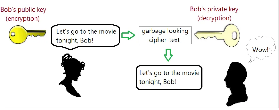
Fig. 2: A simplified illustration of public-key cryptography (for data security).
These are just the basics of how public-key cryptography works. To understand where the
proposed work fits in, one needs to go into the workings of the RSA cryptography
specifically. It does not mean to limit the application of the proposed work (or any that
figure in the technical survey) to just RSA cryptography. The applications go beyond
RSA crypto-systems, but it is just that if anyone were to name one application it would
probably be RSA crypto-systems.
2.5RSA cryptography
Before beginning the description of RSA encryption, it would be helpful to review three
well-known theorems: Fermat’s Little theorem, Fermat’s Extended Theorem, and the
A. Fermat’s Little Theorem
Let p be a prime number, and a be an integer co-prime with p. This can happen if
a is not an integral multiple of p. That is, GCD(a, p) = 1. Note that GCD is the Greatest Common Divisor. Then,
ap−1 = 1 mod p.
B. Fermat’s Theorem Extension
If GCD(p,q) = 1, then pϕ(q) = 1 mod q, where ϕ(q) represents the number of integers less than m that are co-prime with m – which is essentially the Euler-Totient function. The number m is not necessarily prime.
C. Chinese Remainder Theorem
Let p and q be two numbers (not necessarily primes), but such that GCD(p,q) = 1. Then if a = b mod p and a = b mod q, we have,
a = b mod pq.
TheRSAalgorithm
The main intention of the RSA algorithm is to encrypt the message so as to keep it from
everybody except the one with the proper key to decrypt the message. Now, this forms
the core idea of any cryptosystem is the same. Unlike steganography where the very
existence of the message is hid, all cryptographic techniques rely on strong scrambling of
the message. The challenge lies in scrambling the message in such a way that it is
by way of working out the decryption key systematically) within the useful confines of
time and resources.
Rivest, Shamir, and Adleman (RSA being the most common abbreviation for the trio) put
forth an algorithm for carrying out cryptography asymmetrically. In other words, the
RSA algorithm was a public-key technique, and therefore the algorithm does not include
key-sharing.
There are two main stages in carrying out RSA cryptography. The primary part deals
with the generation of private and public keys, followed by the part that deals with the
actual encryption and decryption.
Algorithm for generating the keys:
Step 0: Come up with two large prime numbers (say p1 and p2), not too disparate in size.
Step 1: Let n = pq, and it follows that the Euler-Totient function, ϕ = (p − 1)(q − 1).
Step 2: Choose randomly an integer e (1 < e < ϕ), such that GCD(e,ϕ) = 1. [e is co-prime
with ϕ.]
Step 3: Compute an integer d (1<d< ϕ ) using the Extended Euclidean algorithm, such
that d is the inverse of e modulo ϕ. In other words, ed = 1 mod ϕ.
Next, let us look at the algorithm which specifically represents the encryption and
decryption parts.
Algorithm for encryption and decryption:
A. Encryption
Premise: Alice is the sender, Bob is the recipient.
Step 1: Alice obtains Bob’s public key, {n,e}.
Step 2: The message m is formulated, such that 0 ≤ m < n. Step 3: Send c (ciphertext) = me mod n, to Bob.
B. Decryption
Step 1: Bob receives the ciphertext, c.
CHAPTER III
HISTORICAL OVERVIEW AND TECHNICAL SURVEY
3.1Large-integer multiplication
It is considered best to start this survey of literature in the area of large integer
multiplication via two parts. In the first (which is essentially section 3.1.2), an attempt is
made to make a compilation of the important multiplier designs and multiplication
algorithms chronologically. In the second part (section 3.1.3), an outline of the papers
and patents that make an impact on this research is presented, again chronologically.
Apart from this chronological placement and the sectioning, this thesis introduces a
“Match Grade” for each piece of work that is referred to in this survey chapter. Grade A
indicates a very close resemblance to this research topic and/or a high degree of impact it
bears upon the proposed work. Grade B is work that has been carried out in this area, and
is very relevant to the proposed work. Grade C is for the foundational work that has been
done leading into this area of research, and is distinctly different form central thesis
problem definition.
Finally, after covering both sections of the literature survey, this thesis specifies the
Before beginning with the aforementioned two sections, completeness demands an
introduction of the topic from a distance – so that we better appreciate the scope of the
work and the motivations, for it is very easy to lose track of the broader picture as we
delve into the finer contributions of the many articles showcased in this report. Let us
begin with a bird's eye view of multiplication, and swoop in to the problem statement by
the end of this report.
3.1.1Multiplication and Basic Multipliers
Multiplication at the most basic level is simply accumulating a number upon zero for a
given number of times. The cost of realizing this innocuous looking operation cannot be
underestimated.
Let us define a cost function C(n) which estimates the number of smaller multiplication
and addition operations needed to accomplish the bigger multiplication. Without loss of
generality, and out of customary practice, we can consider that both operands of the
bigger multiplication are both of the same length of n bits. To put the research activity in
this area succinctly, all efforts to optimize multiplication has centered around reducing
the degree and the coefficients of this function, C(n).
The elementary school method of carrying out multiplication may be the easiest to
As an example, consider, A = a1x + a0, and B = b1x + b0. C = A*B = (a1*b1)x2 + (a1*b0 +
b1*a0)x + a0*b0. Expanding the original multiplication this way is indeed the elementary
school method. This method requires 4 smaller multiplication operations, and 3 addition
operations. In general, this method requires n2 multiplications, and (n-1)2 additions. This
can be thought of to be the upper limit of C(n) of all multiplication algorithms.
Since all coefficients are binary in nature, these multiplication operations are realized by
way of building digital circuits. Therefore, reducing the number of gates directly
decreases the chip area, while parallelizing the structure decreases the time delay. There
are many hardware multipliers based on popular algorithms (like the Booth algorithms,
BMK method, Wallace tree approach, and so on), but these work economically only for
small operands. Let us look at some algorithms that are better suited for large integer
multiplication.
3.1.2Fast multiplication algorithms for large integer operands
3.1.2.1Karatsuba Algorithm
[Match Grade: B+]
Put forth by Anatolii Karatsuba [3] in 1962, the basic principle of this algorithm is to
reduce the number of single-digit multiplications needed to achieve an nxn multiplication
– from n2
to m, where m is at most 3nlog23. For the specific case where n is a power of 2,
m reduces to nlog23. Hence the Karatsuba algorithm has an asymptotic complexity of
Θ(n1.585
Consider two numbers of n-digits represented in some base b (which typically is 2), x and
y. Then we can represent them as a sum of smaller segments:
x = x1bp + x0
y = y1bp + y0
It is to be noted that p is less than n, and x0 and y0 are each lesser than bp.
Then,
xy = b2p(x1y1) + bp(x1y0 + x0y1) + (x0y0)
We can replace xy by z, x1y1 by z2, (x1y0 + x0y1) by z1, and x0y0 by z0. Karatsuba replaced
the two multiplications involved in the computation of z1 by a single multiplication
operation and just a few more addition operations (which are way cheaper than
multiplication).
Retaining z2 and z0 as they are, z1 = (x1 + x0)(y1 + y0) – z2 – z0. By doing this, Karatsuba
successfully eliminated one multiplication operation. Though this algorithms works for
any value of n and p, it is to be noted that the value of m hits the minimum when n = 2a
and p = n/2 (where a is a positive integer).
The Karatsuba algorithm is not very useful when dealing with operands of length smaller
than 128 bits [4]. This is a rough number and it depends on the platform being used for
3.1.2.2Toom-Cook Algorithm
[Match Grade: B+]
Now, let us move on to the more general Tom-Cook algorithm (whose special case is the
Karatsuba algorithm) [3]. Introduced first by Andrei Toom in 1963, and subsequently
improved by Stephen Cook in 1966, this algorithm involves splitting the operands into k
smaller numbers of length p each. As we can readily see, Karatsuba algorithm is the case
where k = 2. k = 3 is also a very famous case (generally referred to as Toom-3), and it
operates at a complexity of Θ(n1.465
). At this point, it is also good to observe that the
elementary school method that I have mentioned in section 2 is also a case of Toom-Cook
algorithm with k = 1. And hence, it is sometimes known as Toom-1 as well, and it
operates at Θ(n2
). Since we shall be seeing a much better algorithm next, the
implementation details of this algorithm will not be discussed.
3.1.2.3Schönhage-Strassen Algorithm
[Match Grade: C]
This is not a new algorithm. But surely, this has been one of the most powerful algorithm
since 1971, when it was introduced by Arnold Schonhage and Volker Strassen [5]. The
This algorithms recursively calls the FFT in algebraic rings of size 22^n + 1. Without
going very deep, let us see a quick overview of the working and advantage/disadvantage
of the Schonhage-Strassen algorithm.
Consider two numbers A and B to be multiplied. Let A and B have n digits each. Then,
their cyclic convolution will also have n entries (although every entry need not be a digit
anymore). If carrying is performed leftward from the LSB, then we arrive at the modular
product of A and B.
So what we get is P = A*B mod (bn – 1). However, if we route the procedure via
negacyclic convolution, we get P = A*B mod (bn + 1). The base b is generally 2, hence
this further reduces to,
P = A*B mod (2n + 1). n again is a power of 2, i.e., n = 2k.
The speeding up of the algorithms lies mainly in the employment of Fast Fourier
Transform techniques (FFT) to carry out the Discrete Fourier Transform (DFT).
The method is to simply take the operands A and B to the frequency domain by way of
applying DFT upon them. Let us denote the frequency domain equivalents of A and B by
A' and B' respectively.
Now, A' and B' are multiplied, which we store in P1'. We obtain P1 by applying Inverse
DFT (IDFT) to P1'. Again the trick is to use any popular I-FFT technique. FFT and I-FFT
The primary advantage comes from the speed. But practical Schonhage-Strassen
implementations outdo Toom-Cook algorithm only for huge operand sizes (in the range
of 22^15 to 22^17).
Now, it is time to move on to a survey of papers. We shall start with the early papers that
laid a solid foundation to the concept of fast hardware multipliers. These may not
necessarily have anything to do with large integer multipliers, but they make way for the
development of multipliers. References to them are made chronologically rather than by
importance or impact (for the Match Grade takes care of the latter).
3.1.3 Overview of published and presented articles – foundational, relevant, and/or
recent
[The Match Grades will be given in the references section.]
3.1.3.1The 1960s
As early as 1964, C.S. Wallace [6] realized that multiplication is one of the more
important
operations in the CPU, and he put forth a suggestion to speed up multiplication by
viewing multiplication as addition of a number of summands. He argued that reducing the
number of such summands, and accelerating the formation and addition of those
pseudo-adders (without any carry-chain propagation) in his paper. He also acknowledges the
trade-off between cost and speed as applicable to the multiplier units.
Soon after Wallace's paper, Dadda [7] came up with some schemes for parallel
multipliers in 1965. Dadda made use of parallel (n-input, m-output) counters. He
proposed a two-step approach: First, two numbers whose sum equals the product of the
operands (without carry-chain propagation) are obtained. Then, the product is obtained in
a carry propagating adder.
3.1.3.2The 1970s
Following the interest generated in the 1960s to speed up multiplication (having realized
its importance), the 1970s saw many new ideas to realize digital multiplication – like
parallelization and residue number system.
In 1970, Habibi and Wintz [8] proposed a number of methods for speeding up
multiplication. They also compared those methods on the basis of complexity, cost, and
speed.Their paper described a parallel multiplier – which employed carry-save technique
– for multiplying 10-bit by 12-bit numbers, with a worst case time of 520 ns. Their
reported expenditure on the ICs was under $500! The authors also remark that the
Dadda-method and the carry-save Dadda-method use fewer full adders in comparison to the Wallace
In 1976, Dadda followed up his own work with fast parallel digital multipliers. [9] Early
on in this paper, it is clarified that parallel multipliers come with higher costs and
complexity compared to standard multipliers, but in turn parallel multipliers offer speed.
We shall discuss no more of this simply due to the fact that Dadda himself states in his
paper that the implementation of large parallel counters (needed for large integer
operands) is not feasible in terms of the chip size and the delay produced.
In 1977, Soderstrand and Fields published a paper on Residue Number System (RNS
henceforth) multiplication (followed by an inherent division by a constant integer – to
effectuate multiplication by a fraction) [10]. Except that RNS scheme was used, this
paper has more applications to digital filter design than to present-day cryptography.
3.1.3.3The 1980s
RNS provided the distinct advantage of offering parallelism to circuits because of its
innate ability to cut off carry-propagation chains. Thus RNS seemed to have been
catching up around that time, as can be seen by the 1981 paper on large moduli
multipliers – in which the large moduli multipliers were designed to extend the dynamic
range of the moduli (2n-1, 2n, 2n+1) [11].
In 1983, Gnanasekaran demonstrated that an n-bit operand bit-serial input – bit-serial
output multiplier can be realized using n 5-input adders [12]. This work is not very useful
(i) The output is bit-serial – starting from the LSB. Output starting from MSB
would be more useful.
(ii) The work deals with bit-serial input, whereas my work uses parallel input.
Therefore, Gnanasekaran's approach is a specific case of my intended work.
In the same year, Preparata [13] described a VLSI network to multiply two large integers
of the same length – based on the Discrete Fourier Transform. The operation time is Θ
(√n) and the chip area is Θ (n), where n is the length of each operand. We would not go
any deeper into this paper, since the mere purpose of mentioning this work is to show that
the idea of using DFT for large integer multiplication has been a revisited one (since the
famous Schonhage-Strassen Algorithm).
Five years later in 1988, Hsu et al. [12] compared dual, normal and standard bases-based
VLSI architectures of finite field multipliers. The purpose is to determine which of the
three bases are best from a VLSI implementation viewpoint. To this end, the authors have
taken into consideration:
(i) Berlekamp's dual-basis multiplier,
(ii) Massey-Omura normal-basis multiplier, and (iii) Scott-Tavares-Peppard standard-basis multiplier,
paper deals with finite field multiplication and not with regular multiplication, and this
thesis believes it provides a good insight into the development of multipliers. The authors
concluded that the basis multiplier occupies the smallest chip area, and that the
dual-basis multiplier outperforms the other two as the order of the field employed shoots up.
They noted that the normal-basis multiplier is more efficient when the task at hand
involved computing the inverse of elements, or squaring/exponentiation operations. This
comes at the cost of area as the order of the field scales up. The standard-basis multiplier
has its own set of advantages too – like the lack of need for basis conversion and the ease
of implementation due to the regularity of the structure.
3.1.3.4The 1990s
In 1990, Hartley and Corbett [13] made note in their paper that digit-serial computations
lead to increased efficiency in chip designs. This paper, while not dedicated to
multiplication, has a section on digit-serial multiplication – wherein the authors have
adopted a parallel array multiplier over the Booth multiplier (attributing this choice to
odd operand sizes, and lack of need for the extra speed resulting from usage of the Booth
multiplier – since the paper also talked about other operations running in parallel which
anyway take longer time). The authors remark that though efficient the Wallace-tree
multiplier is not suitable for VLSI implementation. This paper is important in that the
authors notice that digit-serial techniques increase efficiency. But other than that, the
multiplier choice itself is not great – since the authors have looked at the overall system
Ashur et al. [14] in 1996 described a systolic digit-serial multiplier in which the initial
delay (before the LSB of the output appears) is made independent of the number of bits
and the word length. The authors present an architecture wherein the pipelining is
reduced to the bit-level. It is shown that by properly controlling the number of pipelining
stages and the word length, a desirable compromise can be struck between speed and
cost.
The very next year, an article was published [15] that set out to achieve the same result as
above: bit-level pipelining – allowing higher speed with reasonably low chip area.
However, the focus of this paper is not on achieving higher sample speeds, but instead
trading the extra speed for power consumption reduction. They observed that Type-I
multipliers [16] fare better in terms of power consumption for larger digit sizes. In 1998,
Taiwanese researchers Guo and Wang [17] focused on standard-basis multipliers in their
paper on digit-serial systolic multiplier for GF(2m). The authors claim that their proposed
multiplier achieves an output rate of one every ⌈ ⌉ clock cycles – where L is the digit
size. The authors have taken care to keep the maximum propagation delay under check,
as L gets large by introducing increased pipelining.
The claim is that pipelining each basic cell further into S+1 stages reduces the maximum
delay by roughly S+1. Further, the paper states that digit-serial systolic inverters can be
built using 2m-3 proposed multiplier units, and that digit-serial systolic exponentiator units
can be built with 2m-2 of these multiplier units. The mentioned advantage is an improved
3.1.3.52000 Onwards
Three years after Guo and Wang's publication, in 2001, C.H. Kim et al. [20] came up
with a slightly modified version of [17]. It is their claim that their proposed architecture
leads to significant reduction in computational delay at the cost of a slight increase in
hardware complexity. The authors have used the LSB-first multiplication algorithm
described in [21]. The authors further state that the structure of each Processing Element
of their proposed multiplier is simpler than Guo and Wang's.
That very year, C. Visavakul and his colleagues at London's Imperial College published
their work pertaining to reconfigurable multipliers based on digit-serial structure [22]. In
this piece of work, the authors make possible the construction of any 4Mx4N bit
reconfigurable multiplier with Flexible Array Blocks (FAB) and digit-serial techniques.
They have described the FAB as a 4x4 bit reconfigurable building block made of regular
array of adders. The final multiplier is a direct result of a two dimensional cascading of
these basic FABs. The authors have modified the original FAB structure presented in
[23].
In 2003, M. Hutter et al. [24] published their work on versatile and scalable multipliers –
which made use of an efficient degree reducing circuitry interleaved between
The proposed work of the authors is shown to reduce the critical path of the degree
reduction circuit by 1.36 to 3 times (for digit sizes in the range of 4 to 16 bits).
Two years later, in 2005, W. Tang, H. Wu, and M. Ahmadi [25] published their work on
VLSI implementation of bit-parallel word-serial finite field multiplier in GF (2233). The
authors support their decision to use GF (2233) (out of the five NIST recommended fields)
by stating that it is a large enough field to provide sufficient security to cryptographic
applications, while the irreducible trinomial is simple enough to make the multiplication
significantly less complex. The ASIC houses both a multiplier unit and a squarer unit.
The authors have made use the squarer architecture outlined in [26].
3.2Modular multiplication/reduction techniques
A lot of work has been done in this relatively small area of concentration. However, let us
Fig. 3: A brief timeline of the some important works pertaining to
modular reduction geared towards multiplication.
3.2.1Montgomery modular multiplication algorithm
[Match Grade: A]
Algorithm:
Input: X1 (n bits), X2 (n bits), P (n bits)
Step 1: Compute residues ̃1 = (X1*R) mod P, ̃2 = (X2*R) mod P
Step 2: Compute T = ( ̃1 * ̃2); Compute q = (T mod R)*P’ mod R
[Note: ̃ = ( ̃1 * ̃2 * R-1) mod P]
Step 3: ̃ = (T + q*P)/R
Step 4: If ̃ > P-1, then ̃ = ̃ -P
Step 5: Return ̃.
Insight into the working:
Normal modular multiplication involves division by the modulus, in order to bring the
product within the modulus. This division often turns out to be more expensive than the
original multiplication. Therefore, the most basic rationale behind Montgomery’s
algorithm is to avoid that division.
R is chosen to be bigger than P, and the most convenient value that R takes on is an
integer power of 2. Let R = 2g. This makes sure that R is co-prime with P. We see that
this condition is necessary to bring about the expression,
RR-1 – PP’ = 1
Since we have chosen a value bigger than P for R, R-1 < P. Also, P’ < R. Another
advantage of having R as a power of 2 is that shifting and bit masking become extremely
efficient and simple.
The Montgomery algorithm considers the P-residues instead of the actual operands for
the reason that reducing TR-1 modulo P does not require division by P (where T is the
Why the Montgomery algorithm works perfectly well the way it does can be seen in the
following brief illustration:
Consider two operands, x and y. The M-residues of these operands are ̃ and ̃
respectively. These are computed as: ̃ = xR mod M, and ̃ = yR mod M. Let, z = xy
mod M. We can see that z is our desired output. In the same way as ̃ and ~y are defined,
we can have ̃ = zR mod M, i.e., ̃ = xyR mod M = (xR)(yR)R-1 = ̃ ̃R-1 mod M. If we
denote the product of ~x and ̃, with T, then we have, ̃ = TR-1 mod M, and the
Montgomery algorithm presents a fast way to compute this expression.
Now, consider the following:
TR−1 = TRR−1/R = T(PP’ + 1)/R
Let d be some integer. Then,
((TN’ + dR)P + T)/R mod P = (TP’P + dRP + T)/R mod P = (TP’P + T)/R mod P
This means that one could compute TP’ mod R, instead of TP’. Let, q = (T mod R)P’
mod R.
Let, A = (T + qP)/R
Now, it is evident that A < 2P, since T < RP and q < R. Therefore, we need at most one
subtraction to bring A within the modulus P.
Cost analysis:
Computation of the P-residues is definitely an overhead that has plagued the otherwise
excellent Montgomery algorithm. For the cost analysis here, let us pretend to ignore the
residue computation overhead.
Cost to compute q: (T mod R) comes nearly free (because it is merely bit masking – since
R is a power of 2). Then, (T mod R)P’ needs one gxg multiplication. This would be the
cost to compute q.
Cost to compute A: Calculation of qP needs one gx2n multiplication. Apart from that,
computation of A needs one addition, division by R (which is merely a right shift by g
bits), and possibly a subtraction (which can be viewed as addition complexity-wise).
The value of g can be conveniently chosen as 2n+1.
With this choice of g, the Net Cost: 1 (2n+1)x(2n+1) multiplication, 1 (2n+1)x(2n)
multiplication, 1-2 additions, and a few bit masks and shifts. This cost excludes the
P-residue conversions at the input and output.
3.2.2Barrett’s modular multiplication algorithm
[Match Grade: A]
Algorithm:
Input: X (2n bits), P (n bits) [X is the already computed product.]
Output: A = X mod P
Step 0: Pre-compute μ = ⌊ ⌋
Step 2: A = X – ⌊ ⌋*P
Step 3: While A > P-1,
A = A-P
Step 4: Return A
Insight into the working:
The ranges of the operand to be reduced (X), and of the modulus (P) are well defined.
This enables one to make certain pre-computations based on just the range of X, and the
value of P. These types of pre-computations are especially useful when quite a few
modular multiplications are to be performed with the same modulus.
The only pre-computation required for successful modular reduction using the Barrett’s
algorithm is, μ = ⌊ ⌋. One might wonder about the choice of 22n
in the numerator,
but the reason that might best explain this choice would be truncation loss. To understand
what is meant by truncation loss, let us look at an example.
Let n = 10. Then, 2n = 210 = 1024, and 22n = 220 = 1,048,576. Suppose M = 591. (These
are all randomly chosen numbers for the sake of illustration.)
2n/P = 1.73 (A)
⌊ ⌋ = 1 (AT)
22n/P = 1774.24 (B)
⌊ ⌋ = 1774 (B
T)
We can see that there is more information loss when (A) is truncated to get (AT), than the
At the end of this fabricated example, it is natural to feel that it is beneficial to use bigger
numerators (whose effect can always be negated by dividing later by a power of 2), to
minimize the truncation loss. This could be done, but at the cost of having bigger
multiplications while running the Barrett’s algorithm. So, one has to be familiar with the
existence of this trade-off.
The same concept of optimizing truncation loss, while keeping the multiplier size to a
minimum is a challenge not only in the pre-computation step, but also during the
run-time of the algorithm.
So, it all boils down to managing two trade-offs, as we shall see in the following
equation:
q = ⌊⌊ ⌋ ⌋
where, q is the estimate of the quotient.
A = X – qP
Then, P has to be subtracted from A till the result is smaller than P. The number of such
subtractions does not usually exceed two.
The resultant A is the reduction result.
It is not hard to get a feel for the working of the Barrett’s algorithm. The sole intention of
this algorithm is to come up with an estimate of the quotient, without having to divide by
multiplied by 2n/P, and then truncated, the resulting product should be a pretty accurate
estimate of the quotient. This understanding comes from the chain rule. But as we saw
above, the truncation loss is too much when we divide 2n by P. Therefore, we divide
22n/P, truncate it, and later divide the product of μ and ⌊ ⌋ by 2n. The final result is again
truncated, since the estimate of the quotient has to be an integer.
This provides the intuitive explanation of the working of the Barrett’s algorithm.
Cost analysis:
The pre-computation cost (which applies to the computation of μ) is usually not taken to
be part of the cost. However, just for completeness, we can see that it takes a division of a
2n-bit number by an n-bit divisor. If this pre-computation were part of the run-time
computation, it could easily spell disaster for the Barrett’s algorithm.
Run-time cost: Barrett’s algorithm needs 2 kxn multiplications (where k is at most equal
to n).
3.2.3Modified (Folding) Barrett algorithm
[Match Grade: A]
Insight into the working:
The main idea behind the folding Barrett algorithm is to partially reduce the operand X to
X’. This initial reduction is done by the folding. Then, the classical Barrett algorithm is
applied to X’, instead of X. Since X’ is smaller than X, this arrangement brings about
The trade-off one should be wary of is the amount of folding versus run-time
computational cost. There is a point of diminishing returns for the folding mechanism.
What this means is that after this point, the computational effort that goes into folding is
not justified by the reduction in the computational cost of the regular Barrett algorithm
that follows folding.
Let us see how this point can be worked out.
Consider a system which has F folds. For each fold, we need to compute P(i) = ( )
mod P. So, for fold 1 we have P(1) = 21.5n mod P; for fold 2, P(2) = 21.25n mod P; for fold 3,
P(3) = 21.125n mod P, and so on. This leaves the classical Barrett algorithm with a
pre-computation, μ = ⌊ ( )
⌋
A = X(F) - ⌊⌊ ( ) ) ⌋ ( ) ⌋P
X(F) is arrived at in the following way:
LOOP (i = 1 to F)
X(i) = X(i-1) mod ( ) + ⌊ ) ( ) ⌋P(i) , where, X(0) = X.
It is worked out in [29] that the optimum number of folds (F) to minimize the run-time of
the modified Barrett algorithm is 1.44. Since F has to be an integer, it can be taken that it
is not beneficial to fold more than twice, and that at least one fold will yield better results