Estimation of Admixture Proportions: A Likelihood-Based Approach Using
Markov Chain Monte Carlo
Loune`s Chikhi,*
,†Michael W. Bruford*
,‡and Mark A. Beaumont*
,§*Institute of Zoology, Regent’s Park, London NW1 4RY, United Kingdom,†School of Biological Sciences, Queen Mary and Westfield College,
University of London, London E1 4NS, United Kingdom,‡School of Biosciences, Cardiff University, Cardiff CF10 3TL, United Kingdom
and§School of Animal and Microbial Sciences, University of Reading, Reading RG6 6AJ, United Kingdom Manuscript received September 20, 2000
Accepted for publication April 24, 2001
ABSTRACT
When populations are separated for long periods and then brought into contact for a brief episode in part of their range, this can result in genetic admixture. To analyze this type of event we considered a simple model under which two parental populations (P1and P2) mix and create a hybrid population (H). After that event, the three populations evolve under pure drift without exchange duringTgenerations. We developed a new method, which allows the simultaneous estimation of the time since the admixture event (scaled by the population sizeti⫽T/Ni, whereNiis the effective population size of populationi)
and the contribution of one of two parental populations (which we call p1). This method takes into account drift since the admixture event, variation caused by sampling, and uncertainty in the estimation of the ancestral allele frequencies. The method is tested on simulated data sets and then applied to a human data set. We find that (i) for single-locus data, point estimates are poor indicators of the real admixture proportions even when there are many alleles; (ii) biallelic loci provide little information about the admixture proportion and the time since admixture, even for very small amounts of drift, but can be powerful when many loci are used; (iii) the precision of the parameters’ estimates increases with sample size (n⫽50vs. n⫽200) but this effect is larger for theti’s than forp1; and (iv) the increase in precision provided by multiple loci is quite large, even when there is substantial drift (we found, for instance, that it is preferable to use five loci than one locus, even when drift is 100 times larger for the five loci). Our analysis of a previously studied human data set illustrates that the joint estimation of drift andp1can provide additional insights into the data.
D
URING their history, populations can be separated has also been quite common during the process ofdo-mestication and the creation of new breeds. for long periods and then brought into contact
for a brief episode in part of their range, resulting in The interest for admixture estimation and admixed
populations thus ranges from evolutionary to more
ap-genetic admixture (Bernstein 1931; Chakraborty
1986). This process is frequent in human populations plied issues. The study of admixed populations can
pro-vide information on (i) the inheritance of complex ge-where movements have brought together populations
that were historically separated for varying amounts of netic disease and, in particular, the mapping of the genes
involved (ChakrabortyandWeiss1988;McKeigueet
time. This can be seen, for instance, in South America
where many groups are essentially mixed populations al. 2000). In biogeography it could (ii) help identify
the relative contributions of different glacial refugia to containing varying amounts of contributions from
Euro-pean, African, and native American stocks (e.g., Rob- current populations. In conservation biology it could
also (iii) help define which source populations, and in
ertsandHiorns 1965; Chakraborty1986).
Admix-ture occurs widely and in many species and has certainly which proportion, should be used when reintroduction
programs are defined. taken place a great many times since the last glaciations
when populations expanded from different refugia Even though one could use admixture methods to
estimate the relative contributions of subspecies meet-(Taberletet al.1998;Hewitt2000). On a smaller time
scale, humans have caused extensive admixture through ing in hybrid zones, it is important to stress that the
studies of hybrid zones and of admixed populations are transfers of plants and animals, both inadvertently (as
often quite different. Whereas hybrid zone studies deal in the case of commensal species) and deliberately (as
with spatial phenomena, admixture studies usually dis-in restockdis-ing of rivers with nonnative fishes). Admixture
regard this aspect and concentrate on the estimation
of admixture proportions (see, for instance,Goodman
et al.1999 for an example where the difference is ana-Corresponding author:Loune`s Chikhi, Department of Biology,
Uni-lyzed).
versity College London, Wolfson House, 4 Stephenson Way, London
NW1 2HE, United Kingdom. E-mail: [email protected] Recent theoretical advances substantially improved
the ability to use genetic information from present-day lelic loci (similar to many allozymes) or 10-allele loci (similar to microsatellite or mtDNA data). Finally, we populations to draw inferences about past demographic
events (e.g., Slatkin and Hudson 1991; Rogers and applied the method to a published human data set.
Harpending1992;WilsonandBalding1998;
Beau-mont1999). The coalescent theory (Kingman1982a,b)
METHODS
provided population geneticists with both a statistical
framework and a simple way to simulate samples taken The model: The admixture model shown in Figure
from populations evolving under different demo- 1 assumes that two independent parental populations,
graphic models (Hudson 1990). However, until a few P
1and P2, of sizeN1andN2, mixed some timeTin the
years ago, all coalescent-based methods were applied to past (measured in generations) with respective
propor-summary statistics. In practice, the coalescent theory tionsp
1andp2(⫽1⫺p1), creating a hybrid population
was used to simulate genealogical trees under different
H of size Nh. At the time of hybridization, the gene
demographic models and the simulated data sets were
frequency distributions of P1 and P2 are, respectively,
used to estimate the distribution of an appropriate
statis-the two vectorsx1andx2, and that of the hybrid
popula-tic (nA, the number of alleles,He, the expected heterozy- tion isp
1x1⫹p2x2. After admixture, P1, P2, and H evolve
gosity, etc.). Although powerful, these methods were
independently (with no migration) by pure drift (no criticized because they do not make full use of the
ge-mutations) until the present time. Even thoughT, the
netic information present in the allelic distribution
time since admixture (in generations) is the same for (Felsenstein1992). Clearly, any method based on a
the three populations, the time scaled by the effective
transformation of the original data can lead to a loss of size of each population can be different for the three
information and should therefore be less powerful than populations and is thus called
t1 ⫽ T/N1, t2 ⫽ T/N2,
methods that use the probability of observing the exact and
th⫽ T/Nh. The parameters of the model are thus
sample configurations (i.e., the likelihood of the sam- p
1,t1,t2,th,x1,x2. Note thatThompson(1973) analyzed
ple). This is particularly relevant for genetic data where the same model using a Brownian motion
approxima-the information available is inherently limited due to tion to represent drift.
correlation between the data points. A Bayesian approach: We are interested in making
One could naively use coalescent-based simulations inferences about a parameter (or a set of parameters)
to estimate how often a particular allelic configuration ⌿
of a statistical model by using the information pro-is observed. Practically, however, thpro-is pro-is not possible
vided by the observation of the data,D.This is given by
because the number of possible genealogies becomes
a probability density function (pdf), which describes the astronomical very quickly. As a consequence, even for
probability distribution of⌿given the datap(⌿|D). We
moderate sample sizes (n⬎10), the likelihood is
impos-can use Bayes’ theorem to write sible to evaluate by direct simulation. One could also
consider using an analytical approach to derive an
ex-p(⌿|D)⫽ p(⌿)p(D|⌿)
p(D) . (1) pression for the likelihood. Unfortunately, this
expres-sion is practically impossible to solve as soon as the
The first term is the pdf of⌿ before the data are
ob-number of alleles and the sample size become large (see,
tained and is therefore called the prioras opposed to
however,methods).GriffithsandTavare´(1994) and
p(⌿|D), which is theposterior.Practically,p(⌿)
summa-Kuhneret al.(1995) were the first to propose solutions
rizes our belief, knowledge, or lack of knowledge about to this problem using Monte Carlo methods.
⌿. The second term represents the probability of
observ-In this article, we apply a full-likelihood and
coales-ing the data under the statistical model. Seen as a func-cent-based approach to the admixture problem. We
de-tion of⌿,p(D|⌿) (⫽ L(⌿)) is the likelihood function
rive the likelihood function and compare results from
(Edwards1972). The last term represents the probabil-this analytical approach with approximations obtained
ity of the data. It is often impossible to evaluate but is
using the method ofGriffithsandTavare´(1994). We
a constant given the data. As a consequence, this term demonstrate the advantage of the latter. To integrate
can be ignored and we need only to knowp(⌿|D) up
over nuisance parameters in the model (such as the
to this multiplicative constant. When⌿is a set of
param-ancestral gene frequencies), we then use the
Metropolis-eters, we can obtain the distribution of any specific pa-Hastings algorithm (a step for which there are no
ana-rameter by averaging across all others, and this is called lytical results). Because of the large amount of time
the marginal pdf. required, most previous full-likelihood (Bayesian)
meth-By taking a Bayesian (or full-likelihood) approach we ods were tested on small data sets (usually one
popula-consider that all relevant information about the
parame-tion, sample sizeⱕ50). In this study we chose to simulate
ter(s) is contained in the posterior pdf, and we are thus
data sets that are closer to those currently available (i.e.,
interested in the complete distribution rather than in
total sample sizes⫽150 and 600, see below). We tested
point estimates. However, summary statistics such as the performance of our method on a wide range of
Figure1.—The admixture model. We assume a single admixture event,Tgenerations ago (see text). The three populations are allowed to have different sizesN1, N2, and Nh. The contribution of parental population 1 isp1.
about the pdf for comparison and are provided as well. functionp(D|p1,t1,t2,th,x1,x2) can be written as (see
O’Ryanet al.1998 for details) For instance, the standard deviation (SD) is given when
useful because it is a commonly used measure of
disper-p(D|p1,t1,t2,th,x1,x2)⫽p(a1,a2,ah|p1,t1,t2,th,x1,x2)
sion. However, dispersion is better described using the
width between the 5 and 95% quantiles. This is often ⫽
兺
c1,c2,ch
兺
f1,f2,fh
ABC, (2)
referred to as the 95% credible or equal-tail probability
interval (CI or ETPI, respectively). To avoid confusion
where
with the 95%confidenceinterval we use ETPI. For
approx-imately symmetric distributions, using the mean, the A⫽ p(a1|f1)p(a2|f2)p(ah|fh)
median, or the mode provides very similar results.
How-B⫽ p(c1|t1,n1)p(ch|th,nh)p(c2|t2,n2)
ever, for distributions that are highly skewed toward
small values, the mode can be very difficult to estimate. C⫽ p(f1|x1,c1)p(fh|p1x1⫹(1 ⫺p1)x2,ch)p(f2|x2,c2).
This proved particularly true for theti’s. We therefore
a1,a2, andahare the sample frequency counts in
present-decided to use the median that is the most widely used
day samples of P1, P2, and H;f1,f2, andfhare the founder
point estimate (seeGelmanet al.1995 for further
discus-frequency counts in P1, P2, and H;c1,c2, andchare the
sions on the choice of a point estimator), keeping in
number of coalescences in the genealogical history; and mind that it is the full posterior pdf that we regard as
n1,n2, andnhare the sample sizes of P1, P2, and H.
relevant.
The first term (A) was first derived bySlatkin(1996)
The Bayesian procedure requires that we provide a
for two alleles and by Nielsen et al. (1998) for any
prior on all parameters of the model. Although this step
number of alleles (Equation 9; see alsoO’Ryan et al.
may be difficult in some problems, since it involves some
1998 for an independent derivation) and represents the
subjectivity (Gelmanet al. 1995), a lack of knowledge
probability of observing a particular allelic configura-can be represented by a flat prior so that the posterior
tion in a sample given the allelic configuration of the will in fact be proportional to the likelihood function.
founders just after admixture. The second term was Because of this, we also use the term likelihood for
derived byTavare´(1984, Equation 6.1) and represents
posterior pdf in some circumstances. We chose flat
pri-the probability of observingcicoalescence events given
ors forp1,t1,t2, andth. Forx1andx2, we chose a prior
the time (scaled by the effective size) since admixture in which all possible allele frequencies have equal
proba-and the sample sizes. Finally, the third term is specific bility; this is given by a uniform Dirichlet distribution.
to our model and represents the probability of the allelic This choice has the advantage of making no specific
configuration in the founders [the sample size of which assumption on how genetically distant the parental
pop-is given by ni ⫺ ci for i ⫽ {1, 2, h}] given the allelic
ulations are and thereby encompasses any possible
his-distribution in the ancestral parental population and tory of the parental populations.
the amount of admixture. The summation is over the
The full likelihood: However, the posteriorp(p1,t1,
number of coalescent events in the genealogy of each
t2,th,x1,x2|D) [corresponding top(⌿|D) in Equation
founder lineages, and the number of different
fre-quency counts for each sample of this size. p(Sk⫺1|Sk)⫽
(nAi⫺1)
(k⫺m) ifSk⫺1 ⫽Sk⫺Ai, i⫽1 . . .m
⫽0 otherwise
It is, however, computationally expensive to estimate
(6) this likelihood directly, because the number of allelic
(Griffiths and Tavare´ 1994; O’Ryan et al. 1998), configurations among the founders that is compatible
where m is the number of allelic types, Ai is the ith
with the data can be very large. An alternative approach
allele, nAi is the number of Ai alleles in the current
is therefore to use sampling methods to estimate the
state, and Sk⫺Ai means that the allelic configuration
likelihood. Equation 2 can be rewritten in a more
gen-is identical toSkapart from the fact thatnAiis reduced
eral form as
by 1. The waiting time until the next coalescent event
p(D|⌿)⫽
冮
G,cp(D|G)p(G|c)p(c|⌿)dGdc, (3) is sampled from an exponential distribution (Kingman
1982a,b;Hudson1990). The equivalent probability
un-whereGrepresents all possible genealogies and consists der the coalescent model for each step in the chain is
of a sequence of c coalescent events going back from (n
Ai⫺1)/(k⫺1), and thereforep(G|c)/p*(G|c) can be
time 0 to timeTand where the allele frequency count obtained by multiplying at each step the ratio of these
among the lineages is recorded at each event. Following quantities, (k⫺ m)/(k ⫺1). In our model, the chain
the notation of Stephens andDonnelly (2000), the stops when the cumulative coalescence times become
integral denotes summation over all numbers of coales- greater than the time of the admixture event. The state
cent events and allelic configurations at each coalescent at that time represents the allelic configuration among
event. This rewriting becomes helpful because it is possi- the founder lineages and is a random draw from the
ble to sample fromp(G|c)p(c|⌿) using standard meth- ancestral frequencies of the parental populations.
ods of simulation from the coalescent (Hudson1990). Therefore, to have an estimate of the likelihood of the
From the standard theory of Monte Carlo sampling (e.g., sample, it is then necessary to multiply the final
probabil-Ripley 1987) we can then estimate (3) as the average ity [the
兿
(k⫺ m)/(k⫺1)] by the probability ofobserv-ofp(D|G) for each realizedG.Unfortunatelyp(D|G) will ing this founding state, which is a multinomial draw
be 0 for most realizedG.To circumvent this problem we from the ancestral parental frequencies. If a chain has
used the method introduced byGriffithsandTavare´ more coalescent events thann ⫺ k(i.e., giving rise to
(1994), which proved extremely efficient in analyzing fewer thankfounders),p(G|⌿)⫽0 by construction.
the case of pure drift (O’Ryan et al.1998; Beaumont This chain is run a reasonably large number of times
andBruford1999;Ciofiet al.1999; see alsoFelsen- and the likelihood is averaged across these runs. A
com-stein et al.1999 for a review). parison of simulatedvs.analytical results on small data
The method of Griffiths and Tavare´:To circumvent sets and comparing results obtained with different
num-the problem of analyzing all possible genealogies and bers of runs on larger data sets shows that 500 runs is
allelic configurations, Griffiths and Tavare´ (1994) large enough to estimate the likelihood when drift only
used a Monte Carlo approach to evaluate the likelihood is considered (seeappendixandO’Ryanet al.1998).
at specific parameter values; as noted by Felsenstein To summarize, the method of Griffiths and Tavare´
et al.(1999) this is equivalent to importance sampling allows us to calculate the likelihood p(D | p1,t1,t2, th,
(IS; seeRipley1987). In this approach (seeStephens x1,x2) for specific values ofp1,t1,t2,th,x1, andx2. Since
andDonnelly2000 for extensive discussion) Equation we are interested in obtaining the posterior distribution
3 can be rewritten as p(p1,t1,t2,th,x1,x2|D) [equivalent top(⌿|D) in
Equa-tion 1] and, in particular, some of the marginals such
as p(p1 | D), we need a method to sample from the
p(D|⌿)⫽
冮
G,cp(D|G)p(G|c)p*(G|c)p*(G|c)p(c|⌿)dGdc. (4) posterior distribution. Markov chain Monte Carlo (MCMC) is a sampling-based method that enables us
Thus (2) as can be approximated by simulatingKtimes
to do so.
fromp*(G|c)p(c|⌿) and estimating (4) as
Markov chain Monte Carlo methodology:In Monte
Carlo simulations, samplesXi(i⫽1 . . .n) of a random
p(D|⌿)⫽ 1
K1...
兺
Kp(D|G)p(G|c)
p*(G|c) (5) variableXare drawn from a distribution(.) and then
used to evaluate functions ofX.When the distribution
for all realizedGandc.In fact, the scheme of Griffiths of interest is impossible to evaluate either because no
and Tavare´ always guarantees thatp(D|G)⫽1, because closed form is known or because it is difficult to sample
the genealogical history is constructed backward from from, it is possible to construct a Markov chain having
the data as described below. (.) as its equilibrium distribution. One method to do
More specifically, theGandcare sampled according so is by using the Metropolis-Hastings algorithm (
Met-to the following scheme. If we call Sk the state with k ropoliset al.1953;Hastings1970), which is described
lineages, the state Sk⫺1 is chosen (going backward in here. If we call Xt the current state of a Markov chain
the algorithm requires that we first choose a candidate
for the next step of the chain,Xt⫹1, by using a proposal
distributionq(.|Xt). The chain then moves from stateXt
to the candidateXt⫹1with probability
␣ ⫽ min
冢
1,(Xt⫹1)q(Xt/Xt⫹1)(Xt)q(Xt⫹1/Xt)
冣
. (7)
Note that we need only to be able to estimate(.) at
some specific values and up to a multiplicative constant
(i.e., provided by the IS scheme above). If the candidate
state is not accepted the chain remains in its current state and a new candidate state is randomly chosen from the proposal distribution. Provided that some
condi-tions are met (irreducibility of the chain;e.g.,Roberts
1996), the proposal distributionq(.|Xt) is to a large
ex-tent unimportant and the chain will sample from(.)
once equilibrium is reached. Practically the choice of
q(.|Xt) is crucial if one wants the chain to reach equilib-rium in a reasonable amount of time (see below). We applied the MCMC algorithm to the parameter space
defined by our admixture model,i.e., p1, t1, t2, th, x1,
andx2.
Different proposal (or updating) distributions were tested during the development of the method. We
fi-nally updated p1 by taking a normal random deviate
aroundp1with a standard deviation 0.05. We also found
it efficient to updatep110% of the time rather than at
every step. The other parameters were updated the rest
of the time. A lognormal distribution with meantiand
standard deviations⫽1/2
√
3nlocon a log scale was usedfort1,t2, andth, where nlocis the number of loci. The
ancestral parental allelic frequencies were updated by
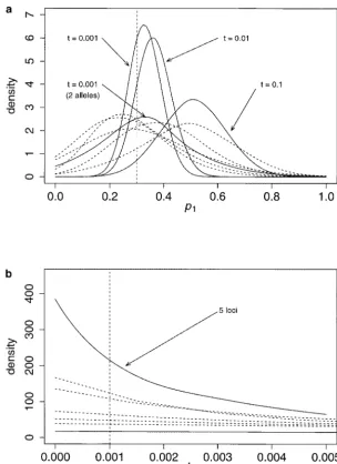
Figure2.—Convergence of the MCMC forp1andth. The
first selecting an allele at random, thus defining a
parti-results of 10 runs are presented forn⫽200 and for the two
tion of two sets of alleles: the allele itself and all the
extreme values ofti(⫽0.001 and 0.1) used in the simulations.
others. A -distribution with parameters v and w was Each curve represents the posterior pdf for 1 run. The curves
then used to update the chosen allele frequency.vwas are close enough to suggest that equilibrium is reached in all
chosen to be 1 while 1/(1 ⫹ w) was equated to the cases. The values of the Gelman convergence statistic were all
between 1.01 and 1.06 for all parameters (see text). The pdf ’s
smallest frequency of the partition (see Appendix in
are obtained using the locfit package for R. The vertical dashed Ciofiet al.1999).
lines represent the values of the parameter with which the
Testing for convergence and analysis of the output: data were simulated. (a) pdf ’s ofp
1forti⫽0.001; (b) pdf ’s
A key issue in MCMC simulation is to determine when ofth forti⫽0.001; (c) pdf ’s ofp1forti⫽0.1; (d) pdf ’s of
thforti⫽0.1.
equilibrium has been reached, i.e., when to stop the
simulation to have a reasonable approximation of the posterior or likelihood curve. This is a serious problem,
since even very long runs that appear to have converged ⬍1.1 (i.e., when the variance between chains is⬍ⵑ5%
may in fact be misleading (seeStephensandDonnelly that observed within chains) are a good indication that
2000 for examples). A number of diagnostic methods equilibrium is reached (seeBeaumont1999).
have been proposed (reviewed byBrooksandGelman We ran 10 independent chains for independent loci
1998), which rely on running either a number of short for each of the three tested values ofti. This was done
chains each with starting points widely dispersed within for loci with 10 alleles and a sample size of 200 genes
the parameter space (Gelmanet al.1995) or one very per population (see next paragraph for the exact
proce-long chain (Raftery and Lewis 1996). We used the dure). In all cases, we found that running the chain for
former method, which is based on the analysis of the 50,000 steps was enough to produce values of the statistic
variance observed for each parameter within (Vw) and ⬍1.1 (see Figure 2, which represents 10 runs forp1and
between (Vb) the chains. This is done by computing thforti⫽0.001 andti⫽0.1). We did not need to repeat
the diagnostic analysis for the smaller sample size (n⫽
50, see below) or number of alleles since equilibrium (see, for instance, the human data set analyzed). Loci with different numbers of alleles can also be used. is reached more quickly.
For each run 10,000 points were collected for all pa- To summarize the principle of our approach, we used
Bayes’ theorem to rewrite the posterior pdf as a function
rameters of the model (i.e., 1 point every 5 steps).
Fol-lowing Beaumont (1999), the first 1000 points (the of a prior and a likelihood. The likelihood was estimated
at specific values of the parameter space using Griffiths “burn-in”) were discarded from the analysis and the
9000 remaining points were used for the convergence and Tavare´’s algorithm and a MCMC was run to obtain
samples from the whole distribution. Finally, we used test and to approximate the likelihood distributions.
For the multiple-loci and the human data sets longer simulated data sets to test the accuracy of the method.
runs were used (see below).
Unless otherwise stated, all statistical analyses were
RESULTS
performed using the R language (Ihaka and
Gentle-man1996). The likelihood curves were estimated using Estimation of admixture proportions from
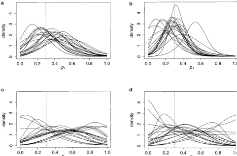
single-locus data:Figure 3 represents the results obtained for
the program Locfit (Loader1996) as implemented in
the locfit package for R (v. 1.0). The convergence diag- the 20 loci of the 10-allele simulations. It shows the
effect of the sample size andtion the estimation of the
nostics used were performed using the coda package
(v. 0.4-7) as implemented for R (ported by S. Plummer admixture parameter p1. The results are also
summa-rized in Table 1 while those of the 2-allele simulations
on the basis of the CODA package byBestet al.1995).
Simulating according to the model: To test the are summarized in Table 2. The numbers given in both tables represent the averages of the medians of each of method, we simulated data sets according to the model
following a coalescent methodology. The two ancestral the pdf ’s of the independent loci and the width of the
95% ETPI across the 20 loci.
allele frequency distributions,x1andx2, of the parental
populations were simulated from two independent flat For all sample sizes and numbers of alleles, the pdf ’s
widen as the time since admixture increases. This is Dirichlet distributions. The allele frequency
distribu-tions of the hybrid populationxhwere then calculated because the genetic information about the admixture
event is gradually eroded by subsequent genetic drift in
asp1x1⫹p2x2. We simulated the number of founders for
the three populations under pure drift using a standard the three populations. Forti⫽0.001 (n⫽50, 10 alleles)
the average SD across the 20 loci ofp1’s posterior pdf ’s
coalescent methodology over the intervalst1,t2, andth,
respectively. The genetic types of the founders of the is 0.184 and increases to 0.198 forti⫽0.01 and to 0.222
forti⫽0.1. The 95% ETPI averaged across loci can be
three populations were then sampled fromx1,x2, and
xh. For each of the populations, a lineage was chosen rather large and ranges from 0.71 to 0.81 astigoes from
0.001 to 0.1 (for then ⫽ 50, 10-allele case, Table 1).
randomly and duplicated until the sample size was
reached. The output of these simulations was fed into This indicates that the number of values that can be
regarded as unlikely is in fact limited when only 1 locus a program implementing our method. Because of the
huge amount of calculations involved by MCMC meth- is used (ⵑ20–30% of thep1values).
The effect of increasing sample size can be seen by ods we had to limit the parameter combinations that
could be analyzed. All simulations were thus performed comparing the left and right sides of Figure 3 and Tables
1 and 2. For ti ⫽ 0.001 the average width of the 95%
withp1⫽0.3 and by considering the same sample size
for the three populations. However, the effect of sample ETPI decreases from 0.71 to 0.56 and the average SD
from 0.184 to 0.144 when the sample size goes from 50 size was investigated by using two different sample sizes
(n⫽50 andn⫽200;i.e., 150 and 600 genes from the to 200. Forn⫽200 the 95% ETPI reaches a valueⵑ0.70
and the average SD becomes 0.184 only fortisomewhere
three populations in total, respectively). Three (scaled)
times since admixture were used in the simulations. For between 0.01 and 0.1 (Table 1). In other words, the
precision is higher forn⫽ 200 than forn ⫽50, even
simplicity, again, the same value was used for the three
ti(i.e., the three populations were of the same size; see, when drift is 10–100 times as large. Note that the effect
of sample size seems particularly strong for smallti
val-however, discussion for a test of the effect of dissimilar
sizes). We usedti⫽0.001, 0.01, 0.1, which for an effec- ues (95% ETPI of 0.56vs.0.70 forti⫽0.001, as opposed
to 0.77vs.0.81 forti⫽0.1). It is thus worth increasing
tive size of 1000 corresponds to 1, 10, and 100
gen-erations of drift, respectively. For each parameter the sample size only ifti is⬍0.01. This means that, as
drift increases, the amount of information that can be
combination 20 independent loci were simulated (i.e.,
corresponding to 20 independent runs of the coalescent extracted aboutp1is quite limited even with large
sam-ples. In such cases, the only solution is to increase the process). We also tested the importance of the number
of alleles by using loci with either 2 or 10 alleles. For number of loci (see below).
The most dramatic factor affecting the estimation of the 2-allele loci, 10 loci were simulated to reduce the
time of analysis. Note that, for real data sets, there are p1seems to be the number of alleles (Figure 4 and Table
2). Two-allele loci seem to provide little information on no limitations whatsoever on the sample sizes. They can
Figure3.—Posterior pdf ’s ofp1for the 10-allele case. Allelic distributions for 20 independent loci were simulated and analyzed using our method. Each curve is the posterior pdf obtained for 1 locus. The vertical dashed lines represent the values of the parameter with which the data were simulated (p1⫽0.3). The parameter combinations presented here are (a) n⫽50, ti ⫽
0.001; (b)n⫽200,ti⫽0.001; (c)n⫽50,ti⫽0.1; (d)n⫽200,ti⫽0.1.
ti. It is clearly preferable to have a single 10-allele locus should be used with caution. Even though these values
indicate that the method is reliable (the estimates ofp1
after 100 times more generations of drift than one
bial-lelic locus. With 2-allele loci it is practically impossible are very close to the real value for bothti⫽0.001 and
0.01 and differ only moderately for ti ⫽ 0.1), some
to exclude any value ofp1as can be seen from the 95%
ETPIs (Table 2), which cover nearly 95% of the possible single-locus pdf ’s can point to very different values
(Fig-ure 3). For instance, when drift is important (ti⫽0.1),
values ofp1even withn⫽200 (i.e., as one would expect
if there were no data). as many as 11 of the 20 pdf’s had a median⬎0.5, 6 of
which were⬎0.6 and 2 of which were⬎0.7 (forn⫽50).
As should be clear from Figures 3 and 4, single point
estimates such as those provided in Tables 1 and 2 Forn⫽200 there were, respectively, six, three, and two
TABLE 1
Summary statistics of the pdf ’s forp1,t1, t2, andthfor the 10-allele case
n⫽50 n⫽200
p1 t1 t2 th p1 t1 t2 th
ti⫽0.001 Median 0.37 0.041 0.031 0.020 0.29 0.022 0.013 0.008
Width 95% 0.71 0.177 0.142 0.097 0.56 0.099 0.069 0.049
ti⫽0.01 Median 0.40 0.046 0.035 0.026 0.28 0.036 0.025 0.017
Width 95% 0.75 0.183 0.150 0.114 0.63 0.135 0.102 0.081
ti⫽0.1 Median 0.50 0.101 0.120 0.126 0.44 0.132 0.095 0.097
Width 95% 0.81 0.337 0.415 0.337 0.78 0.396 0.282 0.233
TABLE 2
Summary statistics of the pdf ’s forp1,t1, t2, andthfor the two-allele case
n⫽50 n⫽200
p1 t1 t2 th p1 t1 t2 th
ti⫽0.001 Median 0.49 0.697 0.697 0.633 0.49 0.677 0.663 0.631
Width 95% 0.94 3.719 3.631 3.552 0.94 3.601 3.570 3.582
ti⫽0.01 Median 0.49 0.657 0.651 0.633 0.50 0.655 0.685 0.613
Width 95% 0.95 3.564 3.535 3.153 0.95 3.539 3.657 3.485
ti⫽0.1 Median 0.50 0.670 0.733 0.692 0.49 0.723 0.668 0.633
Width 95% 0.95 3.649 3.661 3.525 0.94 3.596 3.574 3.512
For each parameter, we give the mean across the 10 loci of the single-locus medians and width of the 95% ETPI.
loci. Clearly, the whole distribution or the 95% ETPI for the correspondingti. In practice this is easily
over-come by introducing a prior on the distribution of the
should be used in place of the point estimates forp1.
When drift increases, it is possible for at least one of corresponding ti. We come back to this point in the
analysis of the human data set. We observed this effect the populations to become fixed for one allele. In such
cases the absence of polymorphism means that the cor- in the two-allele case for a few loci (1 locus forn⫽200
and 7 loci forn⫽50). As a consequence, the averages
responding population had either a very small size or
a very large T. As a result large values of ti become presented take into account only the parameters for
equally likely and the MCMC cannot reach equilibrium which a posterior pdf was available (i.e., between 7 and
10 loci depending on the parameter combination).
Estimation of time since admixture from single-locus data:Figure 5 shows the effect of drift on the estimation
of th. As for p1, the pdf ’s 95% ETPIs increase as ti
in-creases, reaching values ⵑ0.3–0.4 for ti ⫽ 0.1 (in the
10-allele case, Table 1) and even 3.5 for the 2-allele cases (Table 2). In the 10-allele cases, large samples
(n⫽200) provide more information than smaller ones
(n⫽50) even when drift is 10 times as large. However,
we do not observe a greater effect of the sample size
for small ti, which is similar to that observed for p1.
Note that in the 2-allele cases, where the amount of information is very limited, increasing the sample size has virtually no effect (Table 2) and we therefore focus on the 10-allele cases.
Another difference fromp1 pdf’s is that the median
is a rather poor point estimator oftifor small values of
ti whereas it is reasonable forti ⫽ 0.1 (Table 1). It is
possible that because the pdf ’s of the ti are highly
skewed toward zero, the maximum-likelihood estimate (MLE) should be preferred. However, regardless of the choice of a point estimator, the distributions are very wide: the 95% ETPIs are of the same order of magnitude
for all ti’s and are therefore more than two orders of
magnitude larger than the real ti value forti ⫽0.001.
The simplest solution is probably to follow the full-likeli-hood approach and consider the whole distribution rather than point estimates. Indeed, the pdf ’s obtained
forti⫽0.001 andti⫽0.1 are clearly different (Figure
5) even though summary statistics miss the differences.
Figure4.—Posterior pdf ’s of p1 andthfor the two-allele Even if one uses the whole distribution one may won-case. Ten independent loci were used in the two-allele case
der why these 95% intervals are so large and similar for
(see text). (a)pi’s pdf forn⫽200,ti⫽0.001; (b)th’s pdf for
step of the MCMC. In other words, loci are assumed to be independent.
Figure 6a shows the three pdf’s obtained from the five-loci data together (represented by the solid lines). For comparison, the five single-locus pdf’s obtained for
ti⫽0.001 are represented by dashed lines. The increase
in information is such that it is clearly better to use five
loci than one locus even when the drift is⬎100 times
as large. Indeed, the 95% ETPI of the five single-locus
pdf’s varies between 0.58 and 0.74 forp1whereas it is
0.23, 0.27, and 0.47 when ti ⫽ 0.001, 0.01, and 0.1,
respectively. In other words, the uncertainty on the real
value ofp1 is divided by 2 to 3 depending on whether
the amount of drift is equal or 10 times larger. Even when drift is 100 times larger it is still better to have five loci than one locus. To put this into perspective, in a population whose effective size is 1000, admixture will be better estimated with five loci after 100 genera-tions of drift than it would have been with one locus such as mitochondrial DNA just one generation after
the admixture event. The effect ontiis even larger with
a reduction of the 95% ETPI by a factor 3 to 5. Figure 6a also shows another solid line, which was obtained using the information from five biallelic loci together
for ti ⫽ 0.001. Clearly, the pdf is not distinguishable
from the pdf ’s obtained for single loci having 10 alleles. This indicates that biallelic loci such as allozyme loci can provide reasonable amounts of information on
ad-Figure5.—Posterior pdfs ofthfor the 10-allele case. Each mixture events when they are used jointly. If, as appears curve is the posterior pdf obtained for one locus. The following here, five biallelic loci are approximately equivalent to parameter combinations were used: (a)n⫽200,ti⫽0.001; one 10-allele locus, then studies using 40 allozymes such
(b)n⫽200,ti⫽0.1.
as those produced in the last decades might be compara-ble to studies currently using 5–10 microsatellites. This comparison is certainly very rough, but shows that
pre-tivalues, the effect of sampling is no longer negligible
as compared to drift. Indeed, in the 10-allele cases, when cise estimates of admixture proportions can be
esti-mated with very easily obtained genetic markers.
n ⫽ 200 the width of the 95% ETPI is much more
reduced for smallti’s than whenn⫽50 (Table 1). Thus, Figure 6b shows the apparently flat distributions
ob-tained with single-locus data forti⫽0.001. The
distribu-increasing the sample size does provide information on
theti’s even if it does not have a great effect onp1. Note tion for five loci (solid line) shows an improvement but
apart from pointing toward low values ofti the pdf is
that pdf ’s for t1 are usually larger than those for t2,
simply because p1 ⬍ 0.5 (i.e., there is more genetic still flat. As was said earlier, information on the amount
of drift is limited because of the inherent stochastic information on parental population 2). Even though
reasonable amounts of information can be extracted behavior of the coalescent and of other sources of
varia-tion. Note that the appearance of flatness is increased from single-locus data, it appears that this is true when
the admixture event is recent and both the sample size by the scale used to represent the six curves (see Figure
2b where theti’s are represented on another scale).
and number of alleles are large.
Estimation of parameter values from multilocus data: It might be thought that a convenient way of combin-ing the information across loci would be to multiply Multilocus estimation was performed for the 10-allele
case using the data from 5 loci together. This was done the posterior pdf ’s across loci (instead of running the
multiple loci data) and then renormalizing. However,
for one sample size (n ⫽ 50) and three values of ti,
namely 0.001, 0.01, and 0.1. We used the data from these pdf ’s are marginals and the correct procedure
would be to multiply the full pdf (i.e., across all
parame-the first 5 independent loci analyzed for parame-the parameter
combination (i.e., 5 of the 20 loci represented in Figure ters) and then take the marginal. Using the full pdf
from then independent loci is impractical because of
3, a and c, respectively) to compare the single- and
multiple-locus results. The likelihood for multiple loci the very high dimensional density estimation that would
be involved. Therefore, it is necessary to run the MCMC is estimated using Griffiths and Tavare´’s algorithm by
Figure6.—Multiple-locus analysis: multiple-vs. single-locus pdf ’s. The solid lines represent the pdf ’s obtained with the five loci. The dashed lines represent the five pdf ’s obtained for the five inde-pendent loci forti⫽0.001.
with multiple loci, the MCMC runs take longer to con- simulated and analyzed. Figure 7 shows some of these
results for p1 andth. Even though the number of loci
verge than expected on the basis of the number of loci.
For instance, we ran the five-loci data for 350,000 instead analyzed is limited, a number of features are apparent.
First, the precision on p1 (Figure 7, a and c) seems to
of 250,000 steps. Even though multiple-loci data take
longer to analyze, the data produced justify this extra be mostly dependent on the population that has drifted
most (i.e., the largest value ofti) whether it is the hybrid
analysis time. Also, when only single-locus data are
avail-able the whole pdf should be used. (Figure 7a) or parental (Figure 7c) population. Indeed
the 95% ETPI averaged across the 3 loci is 0.68 forth⫽
Effect of dissimilar sizes: Even though the present
method does not require the populations to have the 0.01 and 0.81 forth⫽0.1. These values are within the
values observed for the 20 loci when the threeti’s were
same size, all previous data sets were simulated under
this assumption (the three ti were always equal, see equal to 0.01 and 0.1, respectively (Table 1). Second,
Figure 7, b and d shows that when there is a 100-fold
methods). It is necessary to test the method when the
parental and hybrid populations have been subject to ratio betweenthand botht1andt2 the posterior pdf ’s
become clearly different. When the ratio is 10 then the dissimilar amounts of drift and assess the effect on the
estimation of the parameters. To do this we simulated difference in the posterior pdf ’s is not as obvious and
would certainly require multilocus or large sample data data sets where the two parental populations were always
of the same size and the hybrid was either 10–100 times to be visible. This is because the pdf ’s on ti are wide
even for small ti’s as was shown before (Figure 5 and
smaller (t1 ⫽ t2 ⫽ 0.001, th ⫽ 0.01 or 0.1) or larger
(th⫽0.001 andt1⫽t2⫽0.01 or 0.1). For each of the Table 1). Third, a comparison of Figure 7, a and c
indicates that the pdf ’s for p1 are thinner when the
Figure 7.—Posterior pdf ’s when the hybrid and parental populations have different sizes. Large hybrid(c and d) cases correspond to simula-tions whereth⫽0.001 (t1andt2vary), whileSmall
hybrid(a and b) cases correspond to simulations where t1⫽ t2 ⫽ 0.001 (and th varies). (a) The three solid lines represent the pdf ’s ofp1for three independent loci for whichth ⫽ 0.01 while the three dashed lines correspond to th ⫽0.1; (b) the three solid lines are the pdf ’s ofthfor three independent loci simulated withth⫽0.01 while the dashed lines correspond toth⫽0.1; (c) the three pdf ’s ofp1fort1⫽t2⫽0.01 (solid lines) andt1⫽t2⫽0.1 (dashed lines); (d) as in b but showing the three pdf ’s oft1andt2forth⫽0.01 (solid lines) andth⫽0.1 (dashed lines).
hybrid is subject to little drift than when it is the parental We applied the method to the Jamaican sample
be-cause it is more likely to fit our model than the other populations that are subject to little drift. This is
surpris-ing because in our simulations two out of three popula- samples. The allele frequencies in the three populations
are given in Table 2 (average sample size: Europeans, tions experience large amounts of drift in the “large
hybrid” cases instead of only one in the “small hybrid” n⫽292; Africans,n⫽388; Jamaicans,n⫽186
chromo-somes; Table 3). We ran the data for the nine loci cases.
independently first (for 50,000 steps) to check for loci that could have a very different behavior, perhaps
indi-APPLICATION TO A HUMAN DATA SET
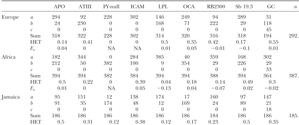
cating selection. Then we ran the data for the nine loci together for 300,000 steps. To check for convergence, We applied the method to a data set published by
Parraet al.(1998). They estimated admixture propor- we ran the chain six times, from different starting points. We also ran one “long” chain for 600,000 steps. The tions of European and African genes in
African-Amer-ican populations from the United States and from first 50,000 steps of each chain (100,000 for the long
one) were discarded and the analysis was done with the
Jamaica using the methods ofLong(1991) and
Chak-raborty (1975). Nine nuclear loci were used (APO, rest of the points after thinning, resulting in 50,000 points per run (100,000 for the long run). Each multilo-AT3-ID, GC, FY-null, ICAM-1, LPL, OCA2, RB2300, and
Sb19.3, most of which are restriction site polymor- cus run took ⵑ1 week on a Pentium 500 Mhz under
Linux.
phisms; seeParraet al.1998 for details). All were
bial-lelic with the exception of GC, which was trialbial-lelic. The The single-locus data analysis was performed for all
loci; but for two loci (FY-null and ICAM), at least one frequencies in the parental populations were obtained
by pulling together three European (England, Ger- parental population was fixed for one of the alleles
(Table 3). The absence of polymorphism despite the many, and Ireland) and three African (one from Central
African Republic, two from Nigeria) samples, respec- large sample sizes means the data are as likely to have
been generated by any large value oftiand the MCMC
TABLE 3
Summary of the human data set
APO ATIII FY-null ICAM LPL OCA RB2300 Sb 19.3 GC n
Europe a 294 92 228 302 146 249 94 289 31
b 24 230 0 0 168 71 222 29 118
c 0 0 0 0 0 0 0 0 45
Sum 318 322 228 302 314 320 316 318 194 292.4
HET 0.14 0.41 0 0 0.5 0.35 0.42 0.17 0.55
Fst 0.04 0 NA NA 0.01 0.03 ⫺0.01 ⫺0.1 0.01
Africa a 182 344 0 284 385 40 359 168 302
b 212 50 382 100 9 354 29 226 29
c 0 0 0 0 0 0 0 0 33
Sum 394 394 382 384 394 394 388 394 364 387.6
HET 0.5 0.22 0 0.39 0.04 0.18 0.14 0.49 0.3
Fst 0.01 0 NA 0.05 ⫺0.13 0.04 ⫺0.07 0.02 ⫺0.02
Jamaica a 95 151 12 138 174 17 160 97 147
b 91 35 174 48 12 169 24 89 21
c 0 0 0 0 0 0 0 0 18
Sum 186 186 186 186 186 186 184 186 186 185.8
HET 0.5 0.31 0.12 0.38 0.12 0.17 0.23 0.5 0.35
The absolute frequencies of one, two, or three alleles (a,b, c) are given for each locus. HET is the expected heterozygosity for each locus in each sample.nis the average sample size.Fstmeasures the differentiation between the different samples of the same continent and was estimated asFst⫽{HT⫺(RHi)/ns}/HT, wherensis the number of samples,Hiis the expected heterozygosity
within samplei, andHTis the total heterozygosity. This estimator is not unbiased but gives an idea of the amount of differentiation between samples within continents.
will not reach equilibrium for the corresponding ti’s, in the estimates are taken into account. Not all of these
factors of variation are taken into account by the two which move to larger and larger values. Practically, one
can introduce a prior on the distribution of ti during other methods. This explains why our SD is larger than
theirs. This also means that these methods underesti-the analysis (a possibility could be to use a flat prior
between 0 and some reasonable value such asti⫽1 or mate the true variance and therefore provide the user
with a misleading impression of precision. We are cur-10) and then use the marginals of the other parameters
of interest. A simpler solution is to use directly the rently testing different methods of admixture estimation
(including that of Long) on simulated data sets and marginals obtained from the run. Note that this
situa-tion disappears when all loci are analyzed together be- find that our method usually performs best (lower mean
square error and more accurate interval estimation;L.
cause largeti’s become unlikely. The seven remaining
loci showed similar results, with GC, the three-alleles Chikhi, R. A. Nichols, M. W. Bruford and M. A.
Beaumont, unpublished results). locus, showing thinner and slightly shifted pdf ’s with
regard to the others (not shown). Therefore, our results, while supporting the point
estimates given byParraet al.(1998), suggest that the
When all loci are used together the estimates of
ad-mixture proportions in the Jamaican sample are very true value of admixture may be within wider bounds
(95% between 1.9 and 14.1%) than suggested by the
similar to those obtained byParraet al. (1998) using
Long’s (1991) and Chakraborty’s (1975) methods, use of Long’s and Chakraborty’s methods. McKeigue
et al.(2000) developed a Bayesian approach to estimate
pointing to an approximate value of p1 ⵑ7% (Figure
8a; see alsoMcKeigueet al.2000). However, a look at individual admixture proportions and applied it to the
same data set, estimating that the 95% ETPI for the the standard deviations obtained with the three
meth-ods shows very different results, i.e., 0.2% (Chakra- Jamaican population was of 6%, that is, larger than that
of Long but smaller than ours. Note thatMcKeigueet
borty), 1.2% (Long), and 3.0% (our method). Our
method seems to indicate a much greater uncertainty al.(2000) used 10 loci instead of the 9 we used, which
makes the comparison difficult.
on the true value ofp1than the two others.
By using a Bayesian approach, we obtain estimates Figure 8 shows the pdf ’s obtained forp1andthin the
European, African, and Jamaican populations, respec-that integrate across all possible gene frequency
distri-butions in the parental populations. The genealogical tively. The most striking result is the fact that th’s pdf
indicates much smaller values for the Jamaican (95% approach allows us to take explicitly into account both
drift in the three populations and the sampling process. ETPI: 0.00032–0.05243) as compared to both the
plain why the Jamaican population seems to have the largest effective size. However, the fact that three other
methods used give similar values forp1 indicates that
this particular assumption should not be problematic.
Indeed, the two methods used byParra et al.(1998)
and that ofMcKeigue et al. (2000) do not make any
assumption on the number of admixture events and the admixture level could have been reached by constant gene flow as well.
In admixture studies, the choice of the parental popu-lations is often crucial. In most cases the exact parental populations cannot be identified with certainty (in fact it may not even be clear whether a “hybrid” population is really admixed). In the present case, the Jamaican population is admixed and the parental populations are known to be European and African. Any pair of samples from both continents would be as good as any other if the level of population differentiation within continents
were low. That is unlikely to be the case, andParraet
al.(1998) were aware of this problem. To circumvent
it, they used a collection of samples from different areas from both Europe and Africa and assumed that the differentiation with other samples would be negligible. This assumption was based on the fact that the different samples they used within each continent were not highly
differentiated. Indeed, theFstestimates we find are
negli-gible (Table 3). However, our analysis indicates that the real ancestral parental populations may have been
Figure 8.—Human data set: admixture in the Jamaican
population. For each parameter, the pdf ’s obtained using misrepresented by present-day parental population
sam-both the long run and the combined sample of the six runs are ples. This is indirectly confirmed by McKeigue et al. shown. In most cases the curves are nearly indistinguishable, (2000) who proposed a test to detect misspecification indicating that equilibrium is reached. (a) pdf ofp1(European
of ancestry-specific allele frequencies. They applied it
contribution to the Jamaican population); (b) pdf ’s of theti
to the data ofParraet al.(1998) for four of the
Afro-for the Jamaican, African, and European populations.
American samples (but not to the Jamaican sample) and found significant results for AT3-ID, OCA2, and GC.McKeigueet al.(2000) were not able to distinguish ropean (95% ETPI: 0.04917–0.67681) populations.
whether it is the African-specific frequencies, the
Euro-Given the inverse relationship betweentiand the size
pean-specific frequencies, or both that are misspecified. of the populations, this result is the opposite to what
A prioriAfrica is most likely to be misrepresented since one would expect. This can be interpreted in different
it is the continent where the greatest amount of genetic ways. First, one could observe that the distributions of
differentiation is observed among human populations,
thetioverlap and therefore may not necessarily indicate
and only samples from Nigeria and the Central African different effective population sizes. This interpretation
Republic were used. Also, as noted byParraet al.(1998)
is not satisfactory because the overlap is very limited at
Angola contributed as much as the Bight of Biaffra least between the Jamaican and the European
popula-(currently Nigeria and Cameroon) into the North Ameri-tions. This can be tested by looking at the joint
distribu-can mainland (25% each, see Curtin 1969 inParraet
tion of the three pairs ofti’s. We find indeed thatt1⬎
al.1998). Considering the geographic distance between
th(P⫽0.0035) andt1⬎t2(P⫽0.0134) whereas there
Angola and Nigeria it should be expected that the
sam-is no significant difference betweenthandt2. Also, we
ples used byParraet al.(1998) may not represent the
showed with simulated data sets that clear differences
original variability of the ancestral populations. A similar
in theti’s pdf ’s appear only when the differences are
argument could be made for the European samples, large (see Figure 7, b and d).
which are all Northern European, even though the Another interpretation is that the data were not
gen-amount of differentiation is more limited than in Africa. erated according to the model. A number of
assump-A posteriorithe data point to a larger misrepresentation tions of the model are certainly not met. One could
of European gene frequencies than African. A likely argue that gene flow from European to Jamaican has
contrib-uted disproportionately to the Jamaican gene pool, the cies) that affect the estimation of the parameters. It also allows for the populations to have different sizes and present-day European sample would appear to have
un-dergone a greater degree of drift from the ancestral therefore experience different amounts of drift (
Thomp-son1973 also allows for different effective sizes). Also,
population. Indeed, taking a sample representing
En-it is the first method that provides an estimation of the
gland, Ireland, and Germany may representmore
vari-time (scaled by the population size) since the admixture ability than there really was in the more limited number
event. of European ancestors of Jamaicans.
It is important to note, though, that two important In conclusion, our method indicates that the
Euro-sources of variation were not taken into account by our pean samples used, and perhaps the African samples as
method: gene flow and mutations. Only Bertorelle and well, are unlikely to be representative of the parental
Excoffier’s method considers the latter. The introduc-populations of the Jamaican population. The effect on
tion of mutations to our model is theoretically possible the final admixture estimate is difficult to predict. One
(Griffiths and Tavare´ 1994; Nielsen 1997;
Beau-way to test this is by using the information that is
cur-mont1999) but would slow the estimation of the
likeli-rently available on the geographic origin of the African
hood enormously. In fact, Stephens and Donnelly
slaves and European slave owners who settled in
Ja-(2000) recently showed that when mutations are added, maica. Samples should then be obtained from these
the choice of the IS function can be critical. In particular
areas in proportion to their known contributions.Parra
they give a new IS function, which, when the mutation
et al.(1998) analyzed their data in this way, using as many
rate is high, can be typically orders of magnitude quicker samples as possible. The robustness of these estimates
and more accurate than Griffiths and Tavare´’s. Clearly, should be checked by excluding the samples of one or
the lack of mutations in our model can be seen as a more of the areas alternatively. Although tedious, this
limitation. Indeed, when any of thetiis large, mutations
last step appears very necessary, given the uncertainty
may not be negligible for some markersif the
popula-of admixture estimates and their importance in
epide-tion size is large (indeed,ti⫽T/Ni). However, for small
miological studies, to cite one example.
populations, mutations will be negligible even for large
ti’s. Therefore, the method should be used with caution
when the admixture event occurred over a time scale
DISCUSSION AND CONCLUSION
comparable to 1/, whereis the mutation rate of the
A number of methods have been developed to esti- marker used. Our aim in this article was to test the effect
mate admixture proportions sinceBernstein’s (1931) of a number of important factors (i.e., the number of
seminal paper (see review byChakraborty1986). Most alleles, loci, and varying sample and effective population
of them usually neglect stochastic effects apart from the sizes). The maximum amount of drift simulated was 0.1,
sampling of the hybrid population. Exceptions include which is much smaller than the expected fixation time of
the early work of Thompson (1973), who introduces 2. Note that other available methods take into account
drift in the estimation of the population frequencies, neither mutations (apart from Bertorelle and
Excof-orLong(1991), who takes into account sampling error fier’s) nor drift in all populations. Also, the advantage
in all populations but drift only in the hybrid popula- of considering pure drift is that we make no assumption
tion. Recently, BertorelleandExcoffier(1998) in- on the mutation model that generated the variation
troduced a number of improvements by (i) explicitly observed in the ancestral parental populations. The
parameterizing the history of the parental populations method can therefore be applied to any type of marker.
prior to the admixture event and (ii) using molecular It is clear that gene flow will also affect the estimates
information (i.e., genetic differences between alleles of admixture. Clearly, our method should be used only
and not only allele frequency information). Recently when there are good reasons to believe that gene flow
also, McKeigue et al. (2000) developed a Bayesian was limited in comparison to the original admixture
method that allows the estimation of admixture for each event (see Bertorelle and Excoffier 1998).
Practi-individual and the distribution of Practi-individual admixture cally, one can argue, as noted by Chakraborty and
oth-in the population. This method does not take a genea- ers, that the admixture proportion estimated by most
logical approach, does not consider drift, and is cur- methods is in fact the result of the cumulative effect of
rently limited to biallelic loci. However, it could be ex- gene flow across generations. It is probable that this will
tended to multiple-allele loci easily (McKeigue et al. be the same with our method but since this was not
2000) and could also take into account some stochas- tested thoroughly, admixture estimates should be used
ticity in the ancestry-specific allele frequencies within with care when they could be the result of continuous
the present-day admixed population (P. M. McKeigue, gene flow. Other methods that estimate gene flow should
personal communication). then be used instead (e.g.,BeerliandFelsenstein1999).
The method presented here takes into account most Another source of error in the estimation of
admix-sources of variation (sampling and drift in all popula- ture proportions is the problem of nonrepresentative