ABSTRACT
SIMMONS, CODY WEBSTER. Puncture Evolution with the Generalized Harmonic Formulation of Einstein’s Equations. (Under the direction of Dr. J. David Brown.)
©Copyright 2014 by Cody Webster Simmons
Puncture Evolution with the Generalized Harmonic Formulation of Einstein’s Equations
by
Cody Webster Simmons
A dissertation submitted to the Graduate Faculty of North Carolina State University
in partial fulfillment of the requirements for the Degree of
Doctor of Philosophy
Physics
Raleigh, North Carolina 2014
APPROVED BY:
Dr. John Blondin Dr. Stephen Reynolds
DEDICATION
BIOGRAPHY
ACKNOWLEDGEMENTS
I would like to thank my advisor David Brown for all of his help. His expertise in the field of numerical relativity has been invaluable, as has been his dedication to helping me finish my graduate studies. His ability to explain (and sometimes explain again) difficult concepts has greatly helped me through my graduate career. I especially appreciate how he has stuck with me even when the progress in my research was slow at times.
I am thankful for all of the teaching opportunities that were available to me at NC State. Not only did they prove to be enjoyable, but without the funding these positions provided, I would never have been able to complete my graduate studies. Thank you to everyone who helped in affording me these opportunities.
I would like to thank my parents, Brenda and Darrell Simmons for instilling in me the drive to succeed and for teaching me to not be afraid of attempting difficult tasks. Without their love, encouragement, and support I would not be the person I am today.
TABLE OF CONTENTS
LIST OF FIGURES . . . vii
Chapter 1 Background Theory . . . 1
1.1 Einstein’s Equations . . . 1
1.2 Synchronization . . . 2
1.2.1 Hypersurfaces . . . 2
1.2.2 Foliations . . . 2
1.3 3+1 Decomposition . . . 3
1.3.1 Metric in 3+1 Coordinates . . . 3
1.3.2 Extrinsic Curvature of Hypersurface . . . 5
1.3.3 Gauss-Codazzi Equations . . . 5
1.4 3+1 Evolution and Constraint Equations (ADM Formulation) . . . 8
1.4.1 ∂tγij . . . 8
1.4.2 Hamiltonian Constraint . . . 10
1.4.3 Momentum Constraint . . . 10
1.4.4 ∂tKij . . . 10
1.4.5 ADM equations . . . 12
1.5 BSSN formulation . . . 12
1.5.1 ∂tϕ. . . 13
1.5.2 ∂tK . . . 13
1.5.3 ∂t˜γij . . . 14
1.5.4 ∂tA˜ij . . . 14
1.5.5 Hamiltionian and Momentum Constraints . . . 15
1.5.6 ∂tΓ˜i . . . 15
1.5.7 BSSN equations . . . 16
1.6 Puncture Method . . . 17
1.6.1 Moving Puncture Method . . . 17
1.6.2 Puncture Initial Data . . . 18
1.6.3 Moving Puncture Gauge . . . 20
1.7 Generalized BSSN . . . 21
1.8 Generalized Harmonic Equations . . . 22
1.8.1 Einstein’s Equations with Generalized Harmonics . . . 23
1.8.2 GH in 3+1 form . . . 23
1.8.3 GH in Conformal Variables . . . 24
1.8.4 Comparison to GBSSN . . . 26
Chapter 2 Generalized Harmonic Evolution . . . 27
2.1 Numerical Simulations Overview . . . 27
2.1.1 Numerical Code . . . 27
2.1.2 What to Look For . . . 28
2.2 Evolution of a Schwarzschild Black Hole . . . 29
2.2.2 Desired Behavior - Convergence . . . 32
2.2.3 Desired Behavior - Stationary Solution . . . 33
2.2.4 Comparison to BSSN . . . 38
2.3 Evolution of a Black Hole with Spin . . . 43
2.3.1 Numerical Stability . . . 43
2.3.2 Desired Behavior - Convergence . . . 44
2.3.3 Desired Behavior - Stationary Solution . . . 44
2.3.4 Comparison to BSSN . . . 46
2.4 Evolution of a Binary Black Hole System . . . 48
2.4.1 Numerical Stability . . . 50
2.4.2 Desired Behavior - Convergence . . . 50
2.4.3 Desired Behavior - Stationary Solution . . . 51
2.4.4 Comparison to BSSN . . . 53
Chapter 3 Summary and Future Work . . . 59
3.1 Summary . . . 59
3.1.1 Numerical Stability . . . 59
3.1.2 Behavior of Numerical Data . . . 60
3.1.3 BSSN Comparison . . . 60
3.2 Future Work . . . 61
REFERENCES . . . 62
APPENDICES . . . 65
Appendix A Par Files . . . 66
A.1 puncture-GH.par . . . 66
A.2 puncturewithspin-GH.par . . . 75
A.3 binary-GH.par . . . 85
Appendix B Henry2 Configuration Files . . . 100
B.1 henry2.ini . . . 100
B.2 henry2.cfg . . . 102
B.3 henry2.sub . . . 104
B.4 henry2.run . . . 105
LIST OF FIGURES
Figure 1.1 Lapse and shift vector . . . 4
Figure 1.2 Einstein-Rosen bridge . . . 18
Figure 1.3 Puncture initial data . . . 19
Figure 2.1 Mesh refinement for Schwarzschild simulation . . . 30
Figure 2.2 Convergence test forM1 constraint . . . 33
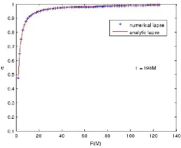
Figure 2.3 Comparison of analytic lapse to numerical lapse on coarsest refinement level att= 198M. AtR≈70 there is some disagreement between the analytic and numerical lapse due to reflection of outgoing modes from the outer boundary. 37 Figure 2.4 Comparison of analytic lapse to numerical laspe on finest refinement level at t = 199.75M. At R ≈0.6 the disagreement is due to insufficient resolution near the puncture. . . 38
Figure 2.5 Killing slices for 1+log slicing condition. . . 39
Figure 2.6 Killing slices for harmonic slicing condition. . . 39
Figure 2.7 GH and BSSN lapse for coarse refinement level of Schwarzschild simulation . 40 Figure 2.8 GH and BSSN lapse for fine refinement level of Schwarzschild simulation . . . 40
Figure 2.9 GH and BSSN trace of extrinsic curvature for coarse and fine refinement levels of Schwarzschild simulation . . . 41
Figure 2.10 GH and BSSN conformal factor for coarse and fine refinement levels of Schwarzschild simulation . . . 42
Figure 2.11 GH and BSSN areal radius verses coordinate radius for fine refinement level of Schwarzschild simulation . . . 43
Figure 2.12 Stationarity of lapse at t=60M and t=99.75M . . . 44
Figure 2.13 Stationarity of K at t=60M and t=99.75M . . . 45
Figure 2.14 Stationarity of ˜γ11at t=60M and t=99.75M . . . 45
Figure 2.15 GH and BSSN lapse for coarse and fine refinement levels for BH with spin . . 46
Figure 2.16 GH and BSSN trace of extrinsic curvature for coarse and fine refinement levels for BH with spin . . . 47
Figure 2.17 GH and BSSN conformal factor for coarse and fine refinement levels for BH with spin . . . 48
Figure 2.18 Mesh refinement for binary BH simulation . . . 49
Figure 2.19 Binary Convergence test for H constraint before merger . . . 50
Figure 2.20 Binary Convergence test for H constraint after merger . . . 51
Figure 2.21 GH evolution of K for a binary black hole system . . . 52
Figure 2.22 Apparent horizons in x-y plane during inspiral . . . 53
Figure 2.23 Common horizons in x-y plane after mergert= 225M . . . 54
Figure 2.24 Real part of Ψ4 for GH and BSSN . . . 55
Figure 2.25 Imaginary part of Ψ4 for GH and BSSN . . . 55
Figure 2.26 Phase shift of Ψ4 for GH and BSSN . . . 56
Figure 2.27 Real part of Ψ4 at high resolution . . . 57
Figure 2.28 Areal radius verses coordinate radius for GH and BSSN . . . 58
Chapter 1
Background Theory
1.1
Einstein’s Equations
Any numerical simulation of a relativistic spacetime starts with Einstein’s Theory of General Relativity. This can be written1 succinctly as
Gµν =(4)Rµν− 1 2γµν
(4)
R = 8πTµν (1.1)
referred to as Einstein’s equations. This can also be written in a trace-reversed form as
(4)R
µν = 8π(Tµν − 1
2gµνT) (1.2)
which, for a vacuum spacetime2, reduces to
(4)R
µν = 0 (1.3)
These equations are the basis for numerical relativity. In this thesis, each of the various for-mulations of Einstein’s equations are written with matter content (Tµν 6= 0). However, each numerical simulation investigated in this thesis simulates a vaccum spacetime and thus Eq. 1.3 effectively describes these spacetimes. The structure of these simulations begins with the idea of synchronization of hypersurfaces in a 4-D spacetime [8, 24, 2, 12].
1
Geometrized units are used where the graviational constant and speed of light G=c=1.
2A vacuum spacetime is one with no matter content, thusT
1.2
Synchronization
Consider spacetime as a Lorentzian manifold. This consists of a 4-D manifoldMand a metric
gof signature (-+++). To set this up as an initial value (Cauchy) problem,Mmust be foliated into a family of spacelike hypersurfaces. Given initial data on one such hypersurface, this data can then be evolved through ”time”. This is a very intuitive approach that easily lends itself to numerical simulations.
1.2.1 Hypersurfaces
A 3-D manifold Σ embedded into the 4-D spacetime manifoldMis a hypersurface. This math-ematical embedding requires that Σ cannot intersect itself. In order for the hypersurface Σ to be spacelike, it must have signature (+++). Given a scalar field t on M, the hypersurface Σ can be considered a level surface of t if t=constant on Σ. For a level surface of t defining Σ, the gradient 1-form ∇t defines the normal to Σ, using the covariant derivative ∇ associated with the spacetime metric g. This means that for any vector v tangent to Σ, < ∇t,v >= 0
(where<> represents an inner product). The vector ∇~t(dual to ∇t) is therefore a vector that is normal to the hypersurface Σ. ∇~t is necessarily timelike if Σ is spacelike.
1.2.2 Foliations
A foliation ofMinto a family of spacelike hypersurfaces Σtsimply means that each hypersurface is a level surface of the scalar fieldt(Cauchy surface). The scalar fieldtis required to be regular, meaning that the gradient oftnever vanishes. This ensures that the normal to Σ never vanishes.
n=−(∇~t·∇~t)−1/2∇~t=−α~∇t (1.4) with associated one form
n=−α∇t (1.5)
and
n·n=−1 (1.6)
1.3
3+1 Decomposition
Start by defining ⊥≡ αn. This introduces a normal vector that is better suited to the scalar fieldt by which the manifold is foliated. This can be seen by
<∇t,⊥>=α <∇t,n>=α <∇t,−α~∇t >=α2(−<∇t, ~∇t >) = 1 (1.7)
where Eq. 1.4 and Eq. 1.6 were used.
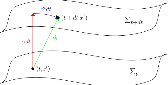
The next step is to introduce a coordinate system (xi) = (x1, x2, x3) on each hypersurface, referred to as spatial coordinates. The coordinate t = constant denotes each hypersurface so that Σt has spacetime coordinates (xα) = (t, x1, x2, x3), referred to as 3+1 coordinates. This gives a basis for the tangent space, Tp(M), of M as (∂α) = (∂t, ∂i). Here, ∂t, referred to as the time vector, is tangent to the curves of constant spatial coordinates connecting each hypersurface. The dual to ∂t is dt = ∇t, so < ∇t, ∂t >= 1. The vector ∂t Lie drags the hypersurface Σt to Σt+δt, so it is a natural evolution vector. If the curves xi = constant are orthogonal to the hypersurface, then ∂t=αn. However, in general this is not the case, so
∂t=αn+β (1.8)
whereβis the shift vector (Figure 1.1). The vectorβis everywhere tangent to the hypersurfaces Σt (β is a spatial vector). Therefore, n and β give a natural 3+1 decomposition of ∂t. This gives
∂t·∂t=−α2+β·β (1.9) so∂t is timelike ifβ·β< α2.
1.3.1 Metric in 3+1 Coordinates The spacetime metricg is defined by
g=gµνdxµ⊗dxν. (1.10) and the induced spatial metric γ, the metric of the family of spacelike hypersurfaces Σt is defined as
γ=γijdxi⊗dxj. (1.11) where⊗ is the outer product.
Σ
tΣ
t+dtαdt ∂t βidt
(t,xi)
(t+dt,xi)
Figure 1.1: Lapse and shift vector
γ(∂i, ∂j) =γij. So
gµν = − α2+β
iβj βj βi gij
!
or
ds2 =gµνdxµdxν =−α2dt2+γij(dxi+βidt)(dxj+βjdt) (1.12) and gµν, the inverse ofg
µν, is written as
gµν = −1/α
2 βj/α2
βi/α2 gij −βiβj/α2 !
The spatial metric γ can also be written as a 4-D tensor
γµν =gµν+nµnν (1.13) or since (nµ) = (−α,0,0,0) and (nµ) = (1/α,−βi/α),
γµν =
βiβi βi βi γij
!
and
γµν = 0 0 0 γij
1.3.2 Extrinsic Curvature of Hypersurface
Now that the metric is written in terms of 3+1 coordinates, the next step is to define the extrinsic curvature of the spacelike hypersurface Σt. First start with the projection operator Xνµ=δνµ+nµnν, which projects tensors onto the spatial hypersurface Σt. It is easily seen that this operator is nothing more than the spatial metric
γνµ=gµν +nµnν. (1.14)
Using this operator, the extrinsic curvature can be defined as
Kµν = −γσµ∇σnν =−(δσµ+nσnµ)∇σnν =−∇µnν−nµnσ∇σnν
= −∇µnν−aνnµ (1.15)
where aν is the acceleration of a Eulerian observer on the hypersurface. The acceleration can be written in terms of the lapse
aν = nµ∇µnν =−nµ∇µ(α∇νt) =−αnµ∇µ∇νt−nµ∇µα∇νt = −αnµ∇
ν(− 1 αnµ) +
1 αnνn
µ∇ µα
= nµ∇
νnµ−αnµnµ∇ν(− 1 α ) +
1 αnνn
µ∇ µα
= αnµnµ∇ν 1 α +
1 αnνn
µ
∇µα=−α 1 α2n
µn
µ∇να+ 1 αnνn
µ
∇µα
= 1
α(∇να+nνn µ ∇µα) = 1 αg µ ν∇µα= 1 αDνα
= Dνlnα (1.16)
This allows Eq. 1.15 to be written as
Kµν =−∇µnν−nµDν(lnα) (1.17)
Even though it is not readily apparent from this equation, the extrinsic curvature is a symmetric tensor Kµν =Kνµ.
1.3.3 Gauss-Codazzi Equations
Gauss Equation
To derive the Gauss equation, start with the Ricci identity for the four dimensional Riemann tensor with respect to the spacetime metricg.
∇α∇βvγ− ∇β∇αvγ=(4)Rγµαβvµ (1.18) The same relation can be written with respect to the spatial metric γ
DαDβvγ−DβDαvγ=Rγµαβvµ (1.19)
where D is the spatial covariant derivative obtained by projecting the spacetime covariant derivative onto the hypersurface. Specifically, this is done by using the spatial metric γ to project each free index onto the spatial hypersurface. As an example, for a four dimensional tensorTν
ρ ,this is defined byDαTδβ =γνβγδργαµ∇µTρν. Examining the first term of Eq. 1.19
Dα(Dβvγ) =γαµγβνγργ∇µDνvρ=γαµγβνγργ∇µ(γνσγ ρ
λ∇σvλ) (1.20) and using ∇µγνσ =∇µgνσ+nν∇µnσ+nσ∇µnν =nν∇µnσ+nσ∇µnν gives
Dα(Dβvγ) = γαµγβνγργ(nσ∇µnνgλρ∇σvλ+γνσnλ∇µnρ∇σvλ+∇µ(nσnν)γλρ∇σvλ +γνσ∇µ(nρnλ)∇σvλ+γσνγ
ρ
λ∇µ∇σvλ)
= γαµγβνγλγ∇µnνnσ∇σvλ+γαµγβσγργ∇µnρnλ∇σvλ+γαµγβσγ γ
λ∇µ∇σv λ
= γµ αγβνγ
γ
λ∇µnνn σ∇
σvλ−γαµγβσγργ∇µnρvλ∇σnλ+γαµγβσγ γ
λ∇µ∇σv λ
= −Kαβγλγnσ∇σvλ−KαγKβλvλ+γαµγβσγ γ
λ∇µ∇σv
λ (1.21)
where the relations γα
βnβ = 0, nλ∇σnλ =−vλ∇σnλ, andγαµγβν∇µnν =−Kβα were used. This means Eq. 1.19 becomes
DαDβvγ−DβDαvγ= (KβγKαλ−KαγKβλ)vλ+γαργβσγ γ
λ(∇ρ∇σv λ− ∇
σ∇ρvλ) (1.22) Now use Eq. 1.18 to get
DαDβvγ−DβDαvγ= (KβγKαµ−KαγKβµ)vµ+γαργβσγ γ λ
(4)
Using this in Eq. 1.19 gives
(KβγKαµ−KαγKβµ)vµ+γαργβσγ γ λ
(4)
Rλµρσvµ=Rγµαβvµ (1.24) or equivalently
γαµγβνγργγλσ(4)
Rσµνρ vλ=Rγλαβvλ+ (KαγKβλ−KβγKαλ)vλ (1.25) This is valid for anyv, so
γµαγβνγργγλσ(4)
Rσµνρ =Rγλαβ+KαγKβλ−KβγKαλ (1.26)
which is known as the Gauss equation. Contracting this relation with γα
γ and using Eq. 1.14 gives
γβνγλσ(4)
Rσν+γβνγλσnµnρ(4)Rρσµν =Rλβ+KKβλ−KβγKγλ (1.27) and using the symmetry of (4)Rρ
σµν
γβνγλσ(4)
Rσν +γαλγβνnµnδ
(4)
Rαδνµ=Rλβ+KKβλ−KβγKγλ (1.28)
which is known as the contracted Gauss equation. Finally, contracting this withγλβto take the trace
γσν(4)
Rσν+gναnµnδ
(4)
Rαδνµ=R+K2−KγλKγλ gσν(4)
Rσν+nσnν(4)Rαδνµ+nνnαnµnδ(4)Rδνµα =R+K2−KγλKγλ
(4)R+ 2(4)R
δµnµnδ=R+K2−KγλKγλ (1.29) and restricting this to the spatial indices for the spatial tensors gives the scalar Gauss equation
(4)R+ 2(4)R
µνnµnν =R+K2−KijKij (1.30)
Codazzi Equation
To derive the Codazzi equation, first start with the Ricci identity with respect to the spacetime metric, Eq. 1.18 and use the unit normal forv
(∇α∇β− ∇β∇α)nγ=(4)Rγµαβnµ (1.31)
Projecting this onto the hypersurface Σ using Eq. 1.14
γγγµγν(4)
and using Eq. 1.15, γα
βnα= 0, γαµγβν∇µnν =−Kαβ, and γργaρ=aγ gives γαµγνβγργ∇µ∇νnρ = γαµγβνγργ∇µ(−Kνρ−aρnν)
= −γαµγβνγργ(∇µKνρ+nν∇µaρ+aρ∇µnν) = −DαKβγ−γαµγργgνβnν∇µaρ−γργaργαµγβν∇µnν = −DαKβγ+a
γK
αβ (1.33)
This means that Eq. 1.32 becomes (using the symmetry of Kαβ) γγ
ργαµγβν(4)Rσµνρ nσ =DβKαγ−DαKβγ (1.34) which is referred to as the Codazzi equation. Contracting this withγα
γ gives DβK−DαKβα = γρµγβνnσ
(4)
Rσµνρ
= (gρµ+nµnρ)γβνnσ(4)
Rσµνρ
= γβνnσ(4)
Rσν+γνβnσnµnρ(4)Rρσµν = γβνnσ(4)
Rσν (1.35)
which is referred to as the contracted Codazzi equation.
1.4
3+1 Evolution and Constraint Equations (ADM
Formula-tion)
The ADM system can be written as a set of evolution equations3 and constraint equations that must be met on each hypersurface4. The original ADM equations were developed by Arnowitt, Deser, and Misner [4], however the equations derived here are based on a rewriting due to York [41]. This rewriting is more stable numerically [2].
1.4.1 ∂tγij
The evolution equation for the spatial metricγ comes directly from the geometry of the foliation (no reference to Einstein’s equations). Start with the Lie derivative of the spatial metric along the normal direction and use the definition of a Lie derivative in terms of covariant derivatives
3The evolution equations consist of time derivatives of the spatial metricγ
ijand the extrinsic curvatureKij.
4
Lnγµν = nσ∇σγµν+γµσ∇νnσ+γνσ∇µnσ
= nσ∇σ(gµν+nµnν) + (gµσ+nµnσ)∇νnσ+ (gνσ+nνnσ)∇µnσ = nσ∇σ(nµnν) +gµσ∇νnσ+gνσ∇µnσ
= (γµσ−gµσ)∇σnν + (γνσ−gσ)ν∇σnµ+∇νnµ+∇µnν = γσ
µ∇σnν+γνσ∇σnµ
= −2Kµν (1.36)
where ∇σgµν = 0 and nσ∇µnσ = 0 was used on the third line. The last line comes from the definition of extrinsic curvature.
Since the goal is actually the Lie derivative along ⊥= αn, the following property of Lie derivatives can be used
Lαnγµν =αLnγµν (1.37) so that
L⊥γµν =−2αKµν (1.38) Now this needs to be converted to a PDE, suitable for a numerical simulation. Using Eq. 1.8 for a given spatial (tangent to Σt) tensor field T
L⊥T =L∂tT − LβT (1.39)
Since the 3+1 coordinate system (xµ) = (t, xi) is adapted to the foliation and thus to the field ∂t, this means that
L∂tT → ∂T
∂t (1.40)
so
L⊥T = (
∂
∂t− Lβ)T (1.41)
Using this relation, Eq. 1.38 becomes
(∂t− Lβ)γij =−2αKij (1.43)
1.4.2 Hamiltonian Constraint
The Hamiltonian constraint is found by starting with the scalar Gauss equation, Eq. 1.30
R+K2−KijKij = (4)R+ 2(4)Rµνnµnν
= 2nµnνGµν (1.44)
and using Einstein’s Equations Eq. 1.1 gives
R+K2−KijKij = 16πnµnνTµν (1.45)
Finally, by defining the energy density, ρ ≡nµnνTµν, the usual form of the Hamiltonian con-straint is given as
H= 0 =R+k2−KijKij−16πρ (1.46)
1.4.3 Momentum Constraint
The momentum constraint is found by starting with the contracted Codazzi relation Eq. 1.35 and using γν
βnσ
(4)R
σν =γβνGσν and Einstein’s Equation, Eq. 1.1, gives DβK−DαKβα = γβνnσGσν
= 8πγβνnσTσν (1.47)
Finally, defining the momentum density, jβ ≡ −γβνnσTσν, and using spatial indices, the usual form of the Momentum constraint is given as
Mi = 0 =DjKij−DiK−8πji (1.48)
1.4.4 ∂tKij
The derivation of the final evolution equation starts with the Ricci Identity applied to n (4)
Rµρνσnρ= (∇ν∇σ− ∇σ∇ν)nµ (1.49)
Contracting it once withnand then projecting the remaining free indices onto the hypersurface Σt usingγ gives
γαµγνβnσ
(4)
and using Eq. 1.17 gives
γαµγβνnσ
(4)
Rµρνσnρ = γανγβnunσ[−∇ν(Kσµ+nσDµ(lnα)) +∇σ(Kνµ+nνDµ(lnα))] = γαµγβνnσ[−∇νKσµ− ∇νnσDµ(lnα)−nσ∇νDµ(lnα) +∇σKνµ
+∇σnνDµ(lnα) +nν∇σDµ(lnα)]
= γαµγβν[−∇νnσKσµ+Kσµ∇νnσ−nσ∇νnσDµ(lnα)−nσnσ∇νDµ(lnα) +nσ∇
σKνµ+nσ∇σnνDµ(lnα) +nσnν∇σDµ(lnα)
= γαµγβν[Kσµ∇νnσ+∇νDµ(lnα) +nσ∇σKνµ+Dν(lnα)Dµ(lnα) nσnν∇σDµ(lnα)]
= =KασKβσ+DβDα(lnα) +γαµγβνnσ∇σKµν+Dα(lnα)Dβ(lnα)] = −KασKβσ+γαµγβνnσ∇σKµν+
1
αDαDβα (1.51)
This can be written in terms ofL⊥Kby using Eq. 1.17 in
∇β(αnα) =nα∇βα+α∇βnα =nα∇βα−αKβα−nβDαα (1.52)
so that
L⊥Kαβ = LαnKαβ =αnµ∇µKαβ+Kµβ∇α(αnµ) +Kαµ∇β(αnµ) = αnµ∇
µKαβ−2αKαµKβµ−nβKαµDµα−nαKβµDµα (1.53) Projecting this onto the hypersurface Σt gives
L⊥Kαβ =αγµαγβνnσ∇σKµν−2αγαµγνβKµσKβσ (1.54)
whereγν
βnν = 0 was used. Solving this for γαµγβνnσ∇σKµν and substituting into Eq. 1.51 gives γαµγβνnσ
(4)Rµ ρνσnρ=
1
αL⊥Kαβ+KασK σ β +
1
αDαDβα (1.55) and using the contracted Gauss relation Eq. 1.28 this becomes
γαµγβν(4)R
µν =− 1
αL⊥Kαβ − 1
αDαDβα+Rαβ +KKαβ−2KασK σ
β (1.56) Finally, solving this for L⊥Kαβ and substituting Einstein’s equations written as Eq. 1.2
L⊥Kαβ = −αγαµγβν
(4)R
µν+αRαβ+αKKαβ−2αKασKβσ−DαDβα
so that
(∂t− Lβ)Kij =α(Rij+KKij−2KikKjk)−DiDjα−8πα(sij−γij(s−ρ)/2) (1.58) wheresij ≡Tij is the spatial stress andρ≡nµnνTµν is the energy density.
1.4.5 ADM equations
In summary, the complete set of ADM equations is
∂⊥γij = −2αKij (1.59a)
∂⊥Kij = α(Rij+KKij−2KikKjk)−DiDjα−8πα(sij−γij(s−ρ)/2) (1.59b)
H = R+K2−KijKij−16πρ= 0 (1.59c)
Mi = DjKij−DiK−8πji= 0 (1.59d)
where∂⊥=∂t− Lβ
1.5
BSSN formulation
Unfortunately the ADM formulation has been shown to be only weakly hyperbolic. This leads to stability issues in numerical simulations. The BSSN formulation is strongly hyperbolic, which means much better numerical stability than the ADM formulation. This is accomplished by taking a conformal decomposition, elevating the contracted connection coefficient Γi to an evolution variable, and splitting the extrinsic curvature Kij into trace and trace-free parts. This formulation was developed initially by Shibata and Nakamura [37] and later compared to the ADM formulation by Baumgarte and Shapiro [7].
Start by defining the spatial metric in terms of a conformal factor5 and conformal metric
γij =ψ4γ˜ij =e4ϕ˜γij (1.60) The physical extrinsic curvature can also be expanded into trace and trace-free parts.
Kij =e4ϕ( ˜Aij + ˜γijK/3) (1.61)
5
Inverting these relations gives the conformal variables as
˜
γij = (γ/γ˜)−1/3γij (1.62a) ˜
Aij = (γ/γ˜)−1/3(Kij−γijK/3) (1.62b) ϕ = 1
12ln(γ/γ˜) (1.62c)
˜
K = K (1.62d)
One last conformal variable is used in the BSSN system, the contracted conformal connection ˜
Γi defined as
˜
Γi≡˜γjkΓ˜i
jk =−∂jγ˜ij (1.63) Lastly, the requirement that ˜γ = ¯γ is set, where ¯γ is the determinant of the background metric (metric of coordinate system being used). From this point forward the background metric is chosen as cartesian, so that ˜γ = ¯γ = 1.
1.5.1 ∂tϕ
Contracting the ADM evolution equation for γij (Eq. 1.59a) withγij gives
γij∂⊥γij =−2αK (1.64)
and using γij∂
⊥γij =∂⊥(lnγ) along withψ=γ1/12=eϕ gives the evolution equation forϕ,
∂⊥ϕ=−
1
6αK (1.65)
Since the density weight ofϕis (1/6)6, the Lie derivative forϕwith respect toβcan be written as
Lβϕ=βk∂kϕ+ 1 6∂kβ
k (1.66)
1.5.2 ∂tK
Similarly contracting the ADM evolution equation for Kij (Eq. 1.59b) withγij gives γij∂
⊥Kij =α(R+K2−2KijKij)−D2α−4πα(3ρ−s) (1.67)
and using γij∂
⊥Kij = ∂⊥K −Kij∂⊥γij = ∂⊥K −Kij∂⊥γij along with the ADM evolution equation for γij (Eq. 1.59a) gives
∂⊥K =α(R+K2)−D2α−8πα[(3ρ−s)/2] (1.68)
Now, substitute the Hamiltonian constraint (Eq. 1.59c) to get
∂⊥K=αKijKij−D2α+ 4πα(ρ+s) (1.69) It is now useful to write the Laplacian of α with respect to the conformal metric.
DiDjα= ˜DiD˜jα−4 ˜D(iαD˜j)ϕ+ 2˜γijD˜kαD˜kϕ (1.70) so that
D2α=e−4ϕ[ ˜D2α+ 2 ˜DiϕD˜iα] (1.71) and using Eq. 1.61 and Eq. 1.71 to write Eq. 1.69 in terms of conformal variables gives
∂⊥K =αA˜ijA˜ij+ 1 3αK
2−e−4ϕ[ ˜D2α+ 2 ˜DiϕD˜
iα] + 4πα(ρ+s) (1.72) Since K is a scalar, the Lie derivative is
LβK =βk∂kK (1.73)
1.5.3 ∂tγ˜ij
The BSSN evolution equation for the conformal metric ˜γij is derived from the ADM evolution equation for the physical metric (Eq. 1.59a) along with Eq. 1.60 and Eq. 1.61. After some simplification this gives
∂⊥γ˜ij =−2αA˜ij (1.74) Since γij is a tensor density of weight -2/3, the Lie derivative is
Lβ˜γij =βk∂k˜γij+ ˜γik∂jβk+ ˜γjk∂iβk− 2 3γ˜ij∂kβ
k (1.75)
1.5.4 ∂tA˜ij
conformal variables.
Rij = ˜Rij+Rϕij = ˜Rij −2 ˜DiD˜jϕ+ 4 ˜DiϕDjϕ˜ −2˜γij( ˜D2ϕ+ 2 ˜DkϕD˜kϕ) (1.76) Now, using Eq. 1.72, Eq. 1.74, Eq. 1.65,Eq. 1.70, and Eq. 1.76 the evolution equation for the trace-free curvature tensor is
∂⊥Aij = αKA˜ij−2αA˜ikA˜kj +e
−4ϕ[αR˜
ij −2αD˜iD˜jϕ+ 4αD˜iϕD˜jϕ
−D˜iD˜jα+ 4 ˜D(iαD˜j)ϕ−8παsij]T F (1.77)
Like the conformal metric, ˜Aij is also a tensor density of weight -2/3, so
LβA˜ij =βk∂kA˜ij+ ˜Aik∂jβk+ ˜Ajk∂iβk− 2
3A˜ij∂kβ
k (1.78)
1.5.5 Hamiltionian and Momentum Constraints
The Hamiltonian and momentum constraints can also be written in terms of the conformal variables as
H= 0 = 2 3K
2
−A˜ijA˜ij+e−4ϕ[ ˜R−8 ˜DiϕD˜iϕ−8 ˜D2φ]−16πρ (1.79) and
Mi= 0 = ˜DjA˜ji − 2
3D˜iK+ 6 ˜A j
iD˜jϕ−8πji (1.80) 1.5.6 ∂tΓ˜i
The derivation of the final BSSN evolution equation starts with the definition of the contracted connection coefficient, Eq. 1.63. Taking the time derivative and using the evolution equation for the conformal metric (Eq. 1.74) but with raised indices, gives
∂tΓ˜i = −∂t∂jγ˜ij =−∂j(2αA˜ij)−∂j(Lβγ˜ij)
= −2(α∂jA˜ij + ˜Aij∂jα)−∂j(βk∂k˜γij−˜γkj∂kβi−γ˜ik∂kβj+ 2 3γ˜
ij∂ kβk) = −2(α∂jA˜ij + ˜Aij∂jα) +βk∂kΓ˜i−Γ˜k∂kβi+ ˜γkj∂j∂kβi
+1 3γ˜
ij∂
j∂kβk+ 2 3Γ˜
i∂
As written, this evolution equation leads to a very unstable numerical simulation. It is necessary to substitute the momentum constraint Eq. 1.80 for the divergence of ˜Aij to give
∂tΓ˜i = 2αΓ˜ijkA˜jk− 4 3α˜γ
ij∂
jK+ 12αA˜ij∂jϕ−2 ˜Aij∂jα+βk∂kΓ˜i−˜γijΓ˜kij∂kβi +˜γkj∂j∂kβi+
1 3γ˜
ij∂
j∂kβk+ 2 3˜γ
jkΓi
jk∂kβk−16παe−4ϕji (1.82) 1.5.7 BSSN equations
In summary, the complete set of BSSN equations
∂⊥ϕ = −
1
6αK (1.83a)
∂⊥˜γij = −2αA˜ij (1.83b)
∂⊥K = αA˜ijA˜ij+ 1 3αK
2
−e−4ϕ[ ˜D2α+ 2 ˜DiϕD˜iα] + 4πα(ρ+s) (1.83c) ∂⊥A˜ij = αKA˜ij−2αA˜ikA˜kj +e
−4ϕ[αR˜
ij−2αD˜iD˜jϕ+ 4αD˜iϕD˜jϕ
−D˜iD˜jα+ 4 ˜D(iαD˜j)ϕ−8παsij]T F (1.83d) ∂tΓ˜i = 2αΓ˜ijkA˜jk −
4 3αγ˜
ij∂
jK+ 12αA˜ij∂jϕ−2 ˜Aij∂jα+βk∂kΓ˜i−γ˜ijΓ˜kij∂kβi +˜γkj∂
j∂kβi+ 1 3˜γ
ij∂
j∂kβk+ 2 3γ˜
jkΓi
jk∂kβk−16παe−4ϕji (1.83e) with Lie derivatives
Lβϕ = βk∂kϕ+ 1 6∂kβ
k (1.84a)
Lβ˜γij = βk∂k˜γij + ˜γik∂jβk+ ˜γjk∂iβk− 2 3γ˜ij∂kβ
k (1.84b)
LβK = βk∂kK (1.84c)
LβA˜ij = βk∂kA˜ij + ˜Aik∂jβk+ ˜Ajk∂iβk− 2 3A˜ij∂kβ
k (1.84d)
and constraints
H= 0 = 2 3K
2−A˜
ijA˜ij +e−4ϕ[ ˜R−8 ˜DiϕD˜iϕ−8 ˜D2φ]−16πρ (1.85a)
Mi = 0 = D˜jA˜ji − 2
3D˜iK+ 6 ˜A j
iD˜jϕ−8πji (1.85b) ˜
Γi−˜γjkΓ˜i
jk = 0 (1.85c)
˜
γ = 1 (1.85d)
˜
1.6
Puncture Method
The BSSN equations are most often used in conjunction with a set of intial data and specific gauge conditions, together referred to as the puncture method. The puncture method is based on the compactification of Brill-Lindquist [10, 30] initial data, developed to handle the singularity present at the location of any BH. Using this initial data, along with a specific set of gauge conditions, this method has become a very successful prescription for evolving 3+1 decomposed spacetimes.
1.6.1 Moving Puncture Method
One major problem inherent in evolving black hole spacetimes is singularities, both coordinate and physical. The static puncture method [16, 1] was developed to deal with these problems and modified later to allow black hole motion relative to the numerical grid, now referred to as the moving puncture method. This approach was developed independently by Campanelli et al.[18, 17] and Baker et al. [5, 6].
Coordinate singularities, such as the one that occurs in the Schwarzschild metric atR= 2M, can be avoided by using horizon penetrating coordinates, such as isotropic coordinates
ds2=−(1− M 2r 1 +M2r)dt
2+ψ4(dr2+r2dΩ2) (1.86)
Horizon penetrating coordinates such as these require a superluminal shift (such as the gamma-driver shift) to keep numerical grid points from falling into the singularity.
There are also coordinate singularites in Brill-Lindquist punture initial data (one for each black hole). This was previously dealt with by using the static puncture method [16, 1], excision [38, 36], or turduckening [11]. However, each of these methods have difficulties, specifically with allowing for black hole motion. The moving puncture method avoids these problems. Movement of the puncture is achieved by using an appropriate non-vanishing shift (such as the gamma-driver shift). Also, finite differences can be taken directly across the puncture (a minimum lapse must be used when puncture is located directly on a numerical grid point). These finite difference calculations introduce large error, but these errors do not propagate outside of the horizon of each black hole. This is due to the fact that they would have to propagate faster than the speed of light in order to affect the region exterior to the horizon. Since puncture evolutions are usually used with hyperbolic formulations of Einstein’s equations (BSSN, 3+1 GH, and others) the physical modes are finite7.
7
Unrelated to the choice of coordinates are singularities involving points where the geometric quantities become infinite, such as at the BH singularity. These infinities can be avoided at first by choosing initial data where the puncture lies in the future. Puncture initial data accom-plishes this by using a non-trivial topology, where each black hole is represented by a wormhole connected to two asymptotically flat spacetimes.
1.6.2 Puncture Initial Data
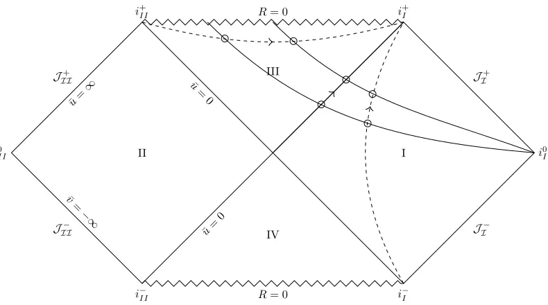
The puncture method uses initial data based on vacuum black holes. This is sometimes referred to as an ”eternal” black hole, as opposed to a ”collapse” black hole (which forms when matter collapses to form the black hole). A pure vacuum solution8 is one in which there is no matter content, i.e.Tµν = 0, ρ= 0, and ji = 0. This greatly simplifies the construction of initial data. This was first investigated by Einstein and Rosen [19], when they searched for a solution of Einstein’s equations with E&M content, absent of any point sources. Their solution is often referred to as an Einstein-Rosen bridge, or ”wormhole” (Figure 1.2). This idea is based on the concept of a time-symmetric vacuum solution (Figure 1.3).
Figure 1.2: Einstein-Rosen bridge
The idea of time-symmetric initial data is used to derive the value of variables on the initial hypersurface, Σt=0. Time-symmetric initial data is a momentarily static solution to Einstein’s equation projected onto the initial hypersurface. It is not physically realistic in the sense that
I II
III
IV i+II
i− II i0 II J+ II ¯ u=
∞ u¯=
0 ¯ u= 0 ¯ v = −∞ J− II
i+I
i− I i0 I J+ I J− I
R= 0
R= 0
Figure 1.3: Puncture initial data
a black hole always has some external forces9 acting on it. This is especially evident for the case of a system with multiple black holes. However, it does provide a good starting point for numerical simulations.
Any initial data must satisfy the hypersurface constraint equations. It is obvious from Eq. 1.59a that a time-symmetric solution requires thatKij = 0. In terms of conformal variables, this means that ˜Aij = 0 andK= 0. For the Hamiltonian constraint, consider it written in terms of the conformal factor,ψ, instead of ϕ(ψ=eϕ). In this form, with the above assumptions for
˜
Aij and K, and absent of any matter content, the Hamiltonian constraint can be written as
H= 0 = 8 ˜D2ψ−R˜ (1.87)
The conformal metric is chosen to be initially flat, ˜γij = δij. This means that ˜R = 0. The Hamiltionian constraint now becomes the Laplace equation forψ.
˜
D2ψ= 0 (1.88)
There are many solutions for this. The most obvious, ψ = 1, recovers Minkowski spacetime with a flat physical metric. The solution ψ = 1 + k
r is the solution used for puncture initial data. This solution, withk= M
2 , corresponds to the spatial part of the isotropic Schwarzschild
9
metric (Eq. 1.86)
dl2 = (1 +M 2r)
4(dr2+r2dΩ2) (1.89) This gives the complete set of puncture initial data for a black hole with no spin or linear momentum as
˜
γij = δij (1.90a)
˜
Aij = 0 (1.90b)
K = 0 (1.90c)
ϕ = ln(1 +M
2r) (1.90d)
˜
Γi = 0 (1.90e)
For multiple black holes, solutions can be superposed. For N black holes,ϕ becomes
ϕ=ln(1 + N X
i=1 mi 2|~r−~ri|
) (1.91)
This is referred to as the Brill-Lindquist solution [10].
Up to this point, the initial data contains black holes with zero spin and linear momentum. Bowen and York [9] developed a relation for the extrinsic curvature ˜Aij that allows for non-zero values of spin and linear momentum.
˜ Aij =
3 2r2[P
inj+Pjni
−(˜γij −ninj)nkPk] + 3 r3[
iklS
knlnj+jklSknlni] (1.92) where Pi and Si are constants in Cartesian coordinates and ni = xi/r is the radial normal vector.
This initial data is usually accompanied by initializing the gauge variables to
α = 1 (1.93a)
βi = 0 (1.93b)
1.6.3 Moving Puncture Gauge
Up until this point, little mention has been made of any gauge conditions which are responsible for choosing the coordinate system in the 3+1 formalism. In principle10, the coordinate system can be freely chosen, and thus the gauge variables (the lapse function α and the shift vector
10
βi) can be freely specified. It is desirable to choose a gauge that is adapted to the geometry of the simulation, that is covariant with respect to spatial transformations on each hypersurface, and is numerically stable.
The gauge condition which have been used very successfully with BSSN simulations starting from puncture data is
∂tα = βi∂iα−2αK (1.94a) ∂tβi = βj∂jβi+
3 4Γ˜
i−ηβi (1.94b)
This is referred to as the ”moving puncture gauge”, composed of the ”1+log” slicing con-dition and the Gamma-driver shift concon-dition. These coordinates seem to be adapted to the geometry of moving puncture simulations using the BSSN formalism in the sense that they are ”symmetry seeking”11[21]. They are also very stable numerically when used in conjunction with the BSSN system. However, the Gamma-driver shift condition is not covariant with respect to spatial transformations.
1.7
Generalized BSSN
The generalized BSSN system developed by Brown [13] addresses the lack of full spatial covari-ance that arises with the standard BSSN system with the moving puncture gauge. It accom-plishes this by writing the BSSN system with moving puncture gauge in terms of tensors with no density weights. This is accomplished by removing the constraint ˜γ = 1 by introducing an evolution equation for ˜γ. The form of this equation is chosen to be ∂t˜γ = 0. The constraint that ˜A= 0 is also removed, so that it is not necessary to enforce this at every time step12. The variable ˜Λi is also introduced to replace the conformal connections ˜Γi, where
˜
Λi = ˜γjk(˜Γijk−Γ¯ijk) = ˜γjk∆˜Γijk (1.95)
11
”Symmetry seeking” refers to the the fact that the coordinates approach Killing coordinates asymptotically, when and if Killing coordinates exist for a given spacetime.
12
. This introduces a new constraint Ci ≡ Λ˜i −∆Γi. With these changes, and assuming that ˜
A= 0 is enforced at every time step, the generalized BSSN equations are
∂⊥˜γij = − 2
3γ˜ijD¯kβ k
−2αA˜ij (1.96a)
∂⊥ϕ =
1 6D¯kβ
k−1
6αK (1.96b)
∂⊥K = αA˜ijA˜ij+ 1 3αK
2−e−4ϕ[ ˜D2α+ 2 ˜DiϕD˜
iα] + 4πα(ρ+s) (1.96c) ∂⊥A˜ij = e−4ϕ[αR˜ij−2αD˜iD˜jϕ+ 4αD˜iϕD˜jϕ−D˜iD˜jα+ 4 ˜D(iαD˜j)ϕ−3παsij]T F
−2
3A˜ijD¯kβ
k−2αA˜
ikA˜kj +αKA˜ij (1.96d) ∂⊥Λ˜i = −γ˜jkCjD¯kβi+ ˜γklD¯kD¯lβi+
2 3γ˜
jk∆˜Γi
jkD¯lβl+ 1 3D˜
i( ¯D
kβk)−2 ˜Aik∂kα +2αA˜kl∆˜Γi
kl+ 12αA˜ik∂kϕ− 4 3αD˜
iK−16παe4ϕji (1.96e)
with Lie derivatives
Lβγ˜ij = βk∂kγ˜ij+ 2˜γk(i∂j)βk (1.97a)
Lβϕ = βk∂kϕ (1.97b)
LβK = βk∂kK (1.97c)
LβA˜ij = βk∂kA˜ij + 2 ˜Ak(i∂j)βk (1.97d)
LβΛ˜i = βk∂kΛ˜i−Λ˜k∂kβi (1.97e)
If the background connection ¯Γi
jk is chosen to be flat, these equations are identical to the standard BSSN equations. The moving puncture gauge becomes
∂tα = βi∂iα−2αK (1.98a) ∂tβi = βjD¯jβi+
3 4Λ˜
i−ηβi (1.98b)
and is now fully spatially covariant.
1.8
Generalized Harmonic Equations
1.8.1 Einstein’s Equations with Generalized Harmonics The definition ofHµ can be written in the form of a constraint equation:
Cµ≡Hµ+ ((4)
Γµσρ−(4)¯
Γµσρ)gσρ (1.99)
Using this definition and writing (4)R
µν in terms of connection coefficients, Eq. 1.2 can be written as
(4)
Rµν− ∇(µCν) = −κ[n(µCν)−gµνnσCσ/2] + 8π(Tµν−gµνT /2) (1.100a)
Cµ = 0 (1.100b)
where κ is a coefficient introduced in front of the new terms on the rhs to control constraint damping [33, 25].
A high degree of hyperbolicity is a necessary condition to allow for stable numerical evolu-tions of a hypersurface Σ with boundaries. The GH equaevolu-tions are symmetric hyperbolic. This is an improvement on the strongly hyperbolic BSSN equations and hints that the GH equations may lead to a stable puncture evolution. This hyperbolicity requires that H⊥ and Hi do not
depend on Kij, π, orρi or any derivatives ofγij, α, orβi [14].
1.8.2 GH in 3+1 form
The generalized harmonic equations, equations (1.100), can be written in 3+1 form by projecting them onto the spacelike hypersurfaces, similar to the derivation of the ADM equations. This splitting is presented in [14]. The results are
∂⊥γij = −2αKij (1.101a)
∂⊥Kij = α[Rij −2KikKjk−πKij]−DiDjα−αD(iCj)−καγijC⊥/2
−8πα[sij −γij(s−ρ)/2] (1.101b)
∂⊥α = α2π−α2H⊥ (1.101c)
∂⊥βi = βjD¯jβi+α2ρi−αDiα+α2Hi (1.101d) ∂⊥π = −αKijKij +DiDiα+CiDiα−καC⊥/2−4πα(ρ+s) (1.101e)
∂⊥ρ = γklD¯kD¯lβi+αDiπ−πDiα−2KijDjα+ 2αKjk∆Γijk +καCi
with constraints
C⊥ ≡ π+K (1.102a)
Ci ≡ −ρi+ ∆Γijkγjk (1.102b)
H ≡ K2−KijKij +R−16πρ (1.102c)
Mi ≡ DjKij−DiK−8πji (1.102d)
Here, several new variables have been introduced. The variables π and ρi are related to the time derivatives of α and βi, respectively. The gauge source vector Hµ has also been split into a spatial scalarH⊥ and a spatial vectorHi. Finally, ∆Γijk = Γjki −Γ¯ijk, where ¯Γijk are the
connection coeffecients built from the background metric.
1.8.3 GH in Conformal Variables
This 3+1 decomposition can now be written in terms of conformal variables to allow easy comparison with the generalized BSSN equations. The conformal variables are defined the same as in equations 1.62 and 1.95. The newly introduced variable ρi can be used in the definition of ˜Λi, such that
˜
Λi = (˜γ/γ¯)1/3ρi+1 6(˜γ/¯γ)
With these definitions, the 3+1 decomposition of the generalized harmonic equations can be written in conformal variables as
∂⊥˜γij = − 2
3γ˜ijD¯kβ
k−2αA˜
ij (1.104a)
∂⊥ϕ =
1 6D¯kβ
k
−16αK (1.104b)
∂⊥K = αA˜ijA˜ij+ 1 3αK
2
−e−4ϕ[ ˜D2α+ 2 ˜DiϕD˜iα] +α(H −KC⊥
−D˜iCi−6Ci∂iϕ)−3ακC⊥/2 + 4πα(ρ+s) (1.104c)
∂⊥A˜ij = e−4ϕ[αR˜ij −2αD˜iD˜jϕ+ 4αD˜iD˜jϕ−D˜iD˜jα+ 4 ˜D(iαD˜j)ϕ−8παsij]T F
−2
3A˜ijD¯kβ
k−2αA˜
ikA˜kj +αKA˜ij −αC⊥A˜ij
+αe−4ϕ[4C(iD˜j)ϕ−Ck∆˜Γk(ij)]T F (1.104d) ∂⊥Λ˜i = ˜γklD¯kD¯lβi+
2 3Λ˜
iD¯ kβk+
1 3D˜
i( ¯D
kβk)−2 ˜Aik∂kα+ 2αA˜kl∆˜Γikl +12αA˜ik∂kϕ−
4 3αD˜
iK+αD˜iC
⊥+
2 3αe
4ϕKCi+καe4ϕCi
−16παe4ϕji (1.104e)
∂⊥α = α2π−α2H⊥ (1.104f)
∂⊥βi = βjD¯jβi+α2Hi+α2e−4ϕ[˜Λi−2 ˜Diϕ−D˜iα/α] (1.104g) ∂⊥π = −αA˜ijA˜ij−
1 3αK
2+e−4ϕ( ˜D2α+ 2 ˜DiϕD˜
iα) +CiD˜iα−καC⊥/2
−4πα(ρ+s) (1.104h)
with constraints
C⊥ = π+K (1.105a)
Ci = −Λi˜ + ∆˜Γijk˜γjk (1.105b)
H = 2 3K
2−A˜
ijA˜ij −16πρ+e−4ϕ[ ˜R−8 ˜DiϕD˜iϕ−8 ˜D2ϕ] (1.105c)
Mi = D˜jA˜ji − 2
3D˜iK+ 6 ˜A j
iD˜jϕ−8πji (1.105d) ˜
A = 0 (1.105e)
1.8.4 Comparison to GBSSN
The differences between the GH and the GBSSN evolution equations only arise in terms pro-portional to the constraints. These differences are
(∂tγ˜ij)GH −(∂tγ˜ij)BSSN = 0 (1.106a) (∂tϕ)GH−(∂tϕ)BSSN = 0 (1.106b) (∂tK)GH−(∂K)BSSN = α(H −KC⊥)−D˜iCi−6Ci∂iϕ)−3ακC⊥/2 (1.106c)
(∂tA˜ij)GH −(∂tA˜ij)BSSN = −αC⊥A˜ij+αe−4ϕ[4C(iD˜j)ϕ−Ck∆˜Γk(ij)]T F (1.106d) (∂Λ˜i)GH −(∂Λ˜i)BSSN = ˜γjkCjD¯kβi−
2 3γ˜
ijC
jD¯kβk+αD˜iC⊥
+2αKγ˜ijCj/3 +καγ˜ijCj (1.106e)
Chapter 2
Generalized Harmonic Evolution
In this chapter, the generalized harmonic (GH) equations in 3+1 form (Eq. 1.104) are used to perform puncture evolutions of several different vacuum spacetimes: a Schwarzschild black hole, a black hole with spin, and a binary black hole system. Until this time, generalized harmonic evolutions involve excising the region around the black hole and typically employ a gauge driver condition, consisting of evolution equations for the gauge source vector Hµ [34, 28]. The simulations in this paper use puncture initial data along with a singularity avoiding gauge, eliminating the need for excision of the black hole. The results of these simulations are analyzed to see if they are numerically stable, if the solutions behave as desired, and how they compare to BSSN simulations of the same spacetimes.
2.1
Numerical Simulations Overview
2.1.1 Numerical Code
All numerical simulations were performed on the Henry2 HPC at NCSU using the Einstein Toolkit [31], an open source code based on CACTUS [23]. The Einstein Toolkit is a modular code, with each module commonly referred to as a thorn. The Einstein Toolkit uses the mesh refinement thornCarpet [35]. Puncture initial data is provided by the Exact thorn for a single non-spinning black hole and by theTwo Puncturesthorn [3] for black holes with spin and binary systems. The Two Punctures thorn provides initial data based on the Bowen-York extrinsic curvature (Eq. 1.92) and for multiple black holes, the Brill-Lindquist solution (Eq. 1.91). The McLachlan vacuum spacetime solver thorn, ML BSSN [15], was used for BSSN simulations. This thorn was developed using Kranc [27], a Mathematica code used to generate numerical codes. The McLachlan thorn was modified (usingKranc) to develop the Generalized Harmonic thorn used for the GH simulations. Fifth order Kreiss-Oliger dissipation was added using the
All spatial derviatives are performed with fourth order finite differencing. The advection terms1 in the evolution equations use upwind stencils for finite differencing. Time integration is completed using the Method of Lines and a fourth order Runge-Kutta algorithm. The constraint damping coefficient κ that appears in the GH equations is set to unity for all simulations. Various files are necessary to use the Einstein Toolkit on the Henry2 HPC at NCSU, including configuration files (Appendices B.1, B.2, and B.5) and scripts (Appendices B.3 and B.4).
2.1.2 What to Look For
Numerical Stability
This requirement simply means that the numerical simulation should run without crashing at least long enough to extract the necessary physics. For numerical simulations in general relativity, this requires the proper formulation, numerical algorithm, choice of gauge, and the implemention of dissipation if necessary.
Desired Behavior
For any numerical simulation, one very important requirement is proper numerical convergence. As the resolution is increased, the solution should approach the exact solution at the proper rate. Without the proper convergence the results of a numerical simulation cannot be fully trusted and therefore have limited practical value.
For a numerical simulation of a stationary spacetime, it is also desirable to choose a gauge such that the numerical solution approaches a stationary solution, specifically a time indepen-dent metric. In order to accomplish this, the slicing condition needs to be chosen such that evolution of the lapse causes the slice to be Lie-dragged along the Killing vector field, which in turn, means the intrinsic geometry of the slice is time-independent. Once this has been ac-complished, the shift condition can be chosen to make the metric components in the chosen coordinates time-independent. This makes∂tthe killing vector for the given spacetime and the coordinates are referred to as ”symmetry seeking”[21].
Comparison to BSSN
It is natural to compare the numerical simulation of a new formulation of Einstein’s equations to pre-existing simulation results based on previously established formulations, in this case the BSSN formulation. Some of the comparisons made include comparing the time slicing, the behavior of grid variables, gravity wave output, and location of apparent horizons.
1
The advection terms are of the formβi∂iv, for a given variablev, which appear in the Lie derivative of the
2.2
Evolution of a Schwarzschild Black Hole
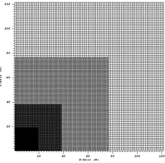
Figure 2.1: Mesh refinement for Schwarzschild simulation
2.2.1 Numerical Stability - Gauge Choice
H⊥ = π+ 2K/α (2.1a)
Hi = e−4ϕ(−Λ˜i+ 2 ˜Diϕ+ ˜Diα/α) + 3 4α2Λ˜
i− η α2β
i (2.1b)
These tests with the puncture gauge led to early instabilities att≈2M. The next gauge tested was the harmonic gauge.
H⊥ = 0 (2.2a)
Hi = 0 (2.2b)
This choice of gauge also showed early instabilities, in this case att≈2M.
These failures led to testing combinations of puncture and harmonic gauges. Using the slicing condition of the puncture gauge (Eq. 2.1a) along with the shift condition of the harmonic gauge (Eq. 2.2b) led to failure aroundt≈1M.
The other possible combination is the harmonic slicing condition with the Γ-driver shift condition.
H⊥ = 0 (2.3a)
Hi = e−4ϕ(−Λ˜i+ 2 ˜Diϕ+ ˜Diα/α) + 3 4α2Λ˜
i
−αη2βi (2.3b)
This gauge choice, referred to as the ”mixed gauge”, proved to be initially successful. The simulation ran without problems until t ≈ 60M at which time the simulation failed. This failure first arose as a violation in the hamiltonian constraint (Eq. 1.102c), which appeared suddenly and grew without bound. This caused growing instabilities in the other grid variables until the simulation failed.
This late instability can be controlled by adjusting the scaling coefficient in the Kreiss-Oliger dissipation. The default value for running the BSSN simulations via the Dissipation thorn is ε= 0.2. By increasingε to 0.35 the simulation ran until t≈130M where it failed again, first appearing as a similar violation of the hamiltonian constraint. Increasing this again toε= 0.5 allowed the simulation to run without failure tot= 200M. A value ofε= 0.8 also allowed for a successful simulation.
conjunction with the GH equations in 3+1 form [14].
2.2.2 Desired Behavior - Convergence
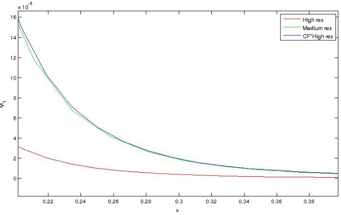
The convergence of the Schwarzschild simulation was tested by comparing the constraint vari-ables (whose exact solution are known), at two different resolutions. The convergence test is based on the expansion of the numerical variables at each resolution and uses the fact that for any constraint variable, C, Cexact = 0.
C∆xlow =Cexact+E(∆x) n+. . . C∆xhigh ≡C∆xlow/f =Cexact+E(∆x/f)n+. . .
wheref = ∆xlow
∆xhigh, n is the order of convergence, and ∆xlow and ∆xhigh are the grid spacing for the numerical simulation. The convergence factor, CF, can be found by
CF = C∆xlow −Cexact C∆xlow/f −Cexact
= E(∆xlow) n E(∆xlow/f)n = E(∆xlow)
n E(∆xlow)n(1/f)n
=fn (2.4)
This test of the convergence factor was completed twice. Initially low and medium resolutions ( ∆xlow = 0.015625M(2M), ∆xmedium= 0.01171875M(1.5M)) were used, but did not exhibit the proper convergence. The proper convergence was obtained with the second test, using the medium and high resolutions, ∆xmedium= 1.5, ∆xhigh = 1.0. For the second test,CF = 1.54= 5.0265 for fourth order accuracy.
Figure 2.2: Convergence test for M1 constraint
2.2.3 Desired Behavior - Stationary Solution
In order for the coordinates chosen by the GH gauge (Eq. 2.3) to be stationary (time indepen-dent), they have to be, by definition, Killing coordinates.
Killing Coordinates
Following the analysis in [22], Killing coordinates are
(∂t)µ=C1ξµ (2.5) whereC1 is an arbitrary constant (C1 6= 0) andξµis a killing vector that is timelike at infinity. This can be contracted with the normalnµ to give the lapse:
α=−nµ(∂t)µ=−C1nµξµ (2.6)
It can also be projected onto the hypersurface to give the shift vector:
βi =C1(⊥ξ)i (2.7)
Schwarzschild Spacetime Killing Coordinates
For a spherically symmetric spacetime, the metric can always be written in the form
ds2 = (β2−α2)dt2+ 2βγrrdrdt+γrrdr2+γθθdΩ2 (2.8)
where β ≡ βr. For convenience, the radial coordinate can be chosen to be proper distance (which means γrr = 1) and γθθ =R2 (where R is the areal radius). This allows Eq. 2.8 to be rewritten as
ds2= (β2−α2)dt2+ 2βdrdt+dr2+R2dΩ2 (2.9) This is the metric for the Killing coordinates (t, r) of the numerical simulation. The Schwarzschild spacetime has a metric
ds2 =−(1−2M R )dT
2+ 1
(1−2MR )dR
2+R2dΩ2 (2.10)
with coordinates (T,R). For coordinates such as these (including Kerr-Schild coordinates), where the Killing vector is ∂T∂ , thegT T component is always given as
gT T = 1− 2M
R (2.11)
The Schwarzschild metric is related to the Killing coordinate metric of the numerical simu-lation (Eq. 2.9) by a coordinate transformation
T = t+F(r) (2.12a)
R = R(r) (2.12b)
which leads to
dT = dt+F0(r)dr (2.13a)
dR = R0(r)dr (2.13b)
where 0 denotes a spatial derivitive with respect to proper distance (r). Substituting Eq. 2.13
into the Schwarzschild metric (Eq. 2.10) leads to the Killing lapse and shift
α = R0 (2.14a)
β = (α2−1 +2M R )
This can also be proven by substituting Eq. 2.9 into Einstein’s equations (Eq. 1.3).
By using the numerical coordinate metric (Eq. 2.9) to solve Eq. 1.59a of the ADM equations forKij and contracting with the spatial metric, the trace of the extrinsic curvature of the slice is found. This solution is
K = 2β R +
β0
R0 (2.15)
This shows the form that the lapse, shift vector, and trace of the extrinsic curvature have for the case of a Schwarzschild spacetime. These can be used to construct an equation for the lapse function as defined by the harmonic slicing condition.
Killing Coordinates with Harmonic Slicing
The harmonic slicing condition can be written as
∂tα=βk∂kα−α2K (2.16) In the case of a stationary solution, ∂tα= 0, leaving
βα0 =−α2K (2.17)
for spherical symmetry. From this equation, Eq. 2.14a, and Eq. 2.15, an equation forα0 can be written as
α0=R00= α 2K
β =R
02(2 R +
β0
βR0) (2.18)
Substituting Eq. 2.14b gives a second order differential equation for R
R00= R
02(2RR02−2R+ 3M)
R(2M−R) (2.19)
As argued in [22], for this solution to be reqular for allR >0, the numerator and denominator must vanish at the same value of r, which is referred to as a regular singular point. The non-trivial solutions to this are
R0 = 0 @ R= 2M (2.20)
R0=±1
2 @ R= 2M (2.21)
Due to Eq. 2.14a, the obvious choice from these solutions isR0 = 1
Analytic Lapse for Harmonic Slicing
Rearranging Eq. 2.18 gives
α0 α =
2R0 R +
β0
β (2.22)
which can be easily integrated to give
α=C2βR2 (2.23)
where C2 is a constant of integration. Using the chosen solution from the previous section, α=R0 = 12 atR= 2M, gives
C2= 1
4M2 (2.24)
so that
α= βR 2
4M2 (2.25)
Finally, substituting Eq. 2.14b into Eq. 2.25 and simplifying givesαas a function of areal radius R.
α= s
R3
(R+ 2M)(R2+ 4M2) (2.26)
Comparison of Numerical Results with Analytic Lapse
Figure 2.4: Comparison of analytic lapse to numerical laspe on finest refinement level at t= 199.75M. At R≈0.6 the disagreement is due to insufficient resolution near the puncture.
2.2.4 Comparison to BSSN
This subsection continues the discussion of killing slices, reviewing the discussion in [22]. The penrose spacetime diagrams of spherical Killing slices for both 1+log (Figure 2.5) and harmonic slicing (Figure 2.6) are shown. For a spherically symmetric spacetime such as the Schwarzschild spacetime, the Killing fields are shown as dashed lines with arrows. The Killing vector that specifies time translation at spatial infinity becomes spacelike inside the horizon (and is thus represented by lines of constant areal radius there).
The 1 +logcondition, used in BSSN simulations, has slices that extend fromi0 I toi
+ II, often referred to as trumpet slices [26]. Ati+II the slices asymptote to constantR≈1.31241M and the slice is therefore tangential to the killing field. This is why the lapse vanishes at the puncture for the 1 +log slicing. The harmonic condition, used in the GH simulations, extend fromi0
I II
III
IV i+II
i− II i0 II J+ II ¯ u=
∞ u¯=
0 ¯ u= 0 ¯ v = −∞ JII−
i+I
i− I i0 I J+ I
JI−
R= 0
R= 0
Figure 2.5: Killing slices for 1+log slicing condition.
I II
III
IV i+II
i− II i0 II J+ II ¯ u=
∞ u¯=
0 ¯ u= 0 ¯ v = −∞ J− II
i+I
i− I i0 I J+ I J− I
R= 0
R= 0
GH simulations, shown on the coarsest (Figure 2.7) and finest (Figure 2.8) refinement levels, exhibit these characteristics.
Figure 2.7: GH and BSSN lapse for coarse refinement level of Schwarzschild simulation
Figure 2.8: GH and BSSN lapse for fine refinement level of Schwarzschild simulation
trace of the extrinsic curvature K (Figure 2.9), and the conformal factorφ (Figure 2.10) show that they look similar for large r, but differ near the puncture.
(a)
(b)
(a)
(b)
Figure 2.10: GH and BSSN conformal factor for coarse and fine refinement levels of Schwarzschild simulation
Figure 2.11: GH and BSSN areal radius verses coordinate radius for fine refinement level of Schwarzschild simulation
2.3
Evolution of a Black Hole with Spin
The second test simulation evolves the spacetime around a spinning BH. The axial symmetry of the spacetime makes this evolution slightly more complicated than the spherically symmetric Schwarzschild BH. The Two Punctures thorn [3] was used to set up the initial puncture data (Eq. 1.90a,Eq. 1.90c-e, and Eq. 1.93) along with the Bowen-York extrinsic curvature (Eq. 1.92). The dimensionless spin parameter was set to s= MSBH2
BH
= 0.6. This simulation was performed with 8 levels of fixed mesh refinement using theCarpet thorn [35]. Each refinement level consists of one octant grid with x, y, z coordinates spanning from 0 to [120, 60, 30, 15, 7.5, 3.75, 1.875, 0.9375] for each grid. The reflection symmetry of the spacetime was provided by the Reflection
Symmetry thorn and the 90◦ rotational symmetry was provided by the RotatingSymmetry90
thorn. The tapering option of the Carpet thorn [35] was also used. The simulation was run with the same medium resolution as the Schwarzschild simulation, 0.01171875M(1.5M) for the finest(coarsest) grid. The gauge conditions used for this evolution were the same mixed gauge conditions that were successful for the Schwarzschild case (Eq. 2.3). The parameter file used for this simulation is shown in Appendix A.2.
2.3.1 Numerical Stability
whether instabilities will occur after this time, so further tuning of the dissipation constant may be necessary for longer runs.
2.3.2 Desired Behavior - Convergence
The convergence of the code for this grid configuration has already been shown for the Schwarz-schild case. Since the resolution, grid structure, and code is exactly the same, it was chosen to not repeat this convergence test. This simulation is closely related to the binary simulation after merger, which is discussed later and tested for convergence.
2.3.3 Desired Behavior - Stationary Solution
Unlike the Schwarzschild case, there is not an analytic lapse to compare the numerical results with. However, stationarity is seen by examining the numerical variables to see that they do settle to a stable solution that does not exhibit large drift2. This can be seen in the evolution of the lapse α (Figure 2.12), the trace of extrinsic curvature K (Figure 2.13), and the x-x component of the conformal metric ˜γ11 (Figure 2.14). There is a difference at large r for these graphs. This is because at t <100M the solution is still settling to the equilibrium state. This movement propagates outward as the simulation advances and the difference is seen to decrease as time advances.
Figure 2.12: Stationarity of lapse at t=60M and t=99.75M
Figure 2.13: Stationarity of K at t=60M and t=99.75M
2.3.4 Comparison to BSSN
The behavior of variables for the BH with spin is very similar to the Schwarzschild simulation. At large r, it was observed that there is little difference between the GH simulation and the BSSN simulation. However, near the puncture there is a difference that closely resembles what is seen in the Schwarzschild simulation. This is seen in the lapse α (Figure 2.15), trace of the extrinsic curvature K (Figure 2.16), and the conformal factor ϕ(Figure 2.17).
(a)
(b)
(a)
(b)
(a)
(b)
Figure 2.17: GH and BSSN conformal factor for coarse and fine refinement levels for BH with spin
2.4
Evolution of a Binary Black Hole System
The third and final test simulation evolves the spacetime around a binary BH system. This is the most complex system tested and shows the robustness of the 3+1 GH formalism. TheTwo
Punctures thorn [3] was used to set up the initial puncture data for both BHs. This consists of
each BH was set to s= 0 and the initial separation of the punctures was set to r = 6M. The initial momentum in the y-direction was set to ±py = 1.3808. This simulation was performed with 7 levels of mesh refinement. Each refinement level consists of one quadrant grid, with x(z) coordinate spanning from 0 to xmax(zmax) and y coordinate spanning from −ymax to ymax, where xmax = ymax = zmax = [120,64,16,8,4,2,1] for each grid (Figure 2.18). The reflection symmetry about the z-axis was provided by theReflection Symmetry thorn and the 180◦
rota-tional symmetry was provided by the SymmetryRotating180 option. This simulation was run with low and high resolutions of 0.0234375M(1.5M) and 0.01953125M(1.25M) respectively for the finest(coarsest) grid. As with the previous two simulations, the same mixed gauge choice (Eq. 2.3) was chosen. The parameter file used for this simulation is shown in Appendix A.3.
2.4.1 Numerical Stability
The first test was run at the low resolution with dissipation constant set to the default BSSN value ofε= 0.2. For this level of dissipation the simulation failed att≈225M. Increasing the dissipation to ε= 0.35 allowed the simulation to run to t= 300M without failure. Increasing the dissipation further to ε= 0.5,0.6, and 0.8 causes failure to occur att≈270M,250M, and 225M, respectively. This differs from the results seen in the Schwarzshild BH and spinning BH cases. In those cases there was a minimum value ofεfor which the simulation would be stable, ε= 0.5 for the Schwarzschild case andε= 0.35 for the spinning BH case. Anything above these values would allow for a numerically stable simulation at least until t≈100M. In the case of the binary system, there seems to be a narrow band of dissipation values (ε≈0.35) that allow for stability. Any value too far above or below this allows for instabilities.
2.4.2 Desired Behavior - Convergence
Since this simulation uses a different grid configuration than the previous two tests, it is prudent to test the convergence once again. For this convergence test, the low resolution of 0.0234375M(1.5M) for the finest(coarsest) grid was used along with the high resolution of 0.01953125(1.25M). For these new resolutions, the ratio of resolutions is f = 1.2 giving the desired convergence factor of CF = 1.24 = 2.0736 for fourth order accuracy. By using this test to compare the constraint variables it can be shown that the desired convergence is obtained both before (Figure 2.19) and after (Figure 2.20) the merger of the BHs.
Figure 2.20: Binary Convergence test for H constraint after merger
2.4.3 Desired Behavior - Stationary Solution
(a) (b) (c)
(d) (e) (f)
(g) (h) (i)
(j) (k)