Sensitivity via the complex-step method for delay differential equations with non-smooth initial data

Sensitivity via the complex-step method for delay

differential equations with non-smooth initial data

H.T. Banks, Kidist Bekele-Maxwell, Lorena Bociu,

Chuyue Wang

Center for Research in Scientific Computation

Department of Mathematics

North Carolina State University

Raleigh, NC 27695-8212

July 31, 2016

Abstract

In this report, we use the complex-step derivative approximation technique to com-pute sensitivities for delay differential equations (DDEs) with non-smooth (discontin-uous and even distributional) history functions. We compare the results with exact derivatives and with those computed using the classical sensitivity equations whenever possible. Our results demonstrate that the implementation of the complex-step method using the method of steps and the Matlab solver dde23 provides a very good approxi-mation of sensitivities as long as discontinuities in the initial data do not cause loss of smoothness in the solution: that is, even when the underlying smoothness with respect to the initial data for the Cauchy-Riemann derivation of the the method does not hold. We conclude with remarks on our findings regarding the complex-step method for com-puting sensitivities for simpler ordinary differential equation systems in the event of lack of smoothness with respect to parameters.

1

Introduction

Sensitivity analysis is of interest in widely diverse topics in mathematics and engineering including parameter selection and identifiability (see [9] and references therein), inverse problem formulations [4, 8], optimal design [12, 13] among others. In this wide range of applications, sensitivities may be desired for model problems coming from real world appli-cations. Often in such cases one encounters non-smooth problems where one does not have analyticity of the response with respect to parameters. Such problems include sensitivity analysis of delay systems with respect to delays (our focus in this note) where in general the solution may lack smoothness in initial histories [14]; PDE problems and sensitivity with respect to boundary parameters (our initial motivation for our investigations of the complex step methods-see [5]), and sensitivities in aggregate data problems where estimated parameters are probability measures [10, Chapter 6].

Delay equations have been used in a wide variety of biological applications as well as in many engineering problems –see for examples the references [1, 2, 3, 6, 7, 16, 17, 18, 19, 22]. Early applications of delay differential equations date back to 1940’s for studies of mechan-ical systems mechanmechan-ical systems by Minorsky [27, 28, 29] and slightly later for studies of population dynamics in biology by Hutchinson [20, 21]. Delay differential equations (DDEs) are particularly interesting because the derivatives of their solutions often have discontinu-ities (see [14] for a theoretical treatment and discussions). This is generally true because the first derivative of a non-constant history function at zero is almost always different from the right derivative of the solution at the initial point. As we shall see below, in addition to the discontinuity at the initial point, discontinuities in derivatives of the initial function tend to be propagated with one degree of smoothness added per time delay interval. Since the complex-step method is derived assuming analyticity, one might expect for the method to fail when it comes to computing the sensitivity with respect to the time lag τ. But the results for these examples show that the complex-step method approximates the sensitivities accurately up to a critical step size (hcrit) in certain cases even in lack of smoothness with

respect to the parameters.

In sensitivity analyses, we study how the output of a model is affected by its inputs such as parameters and initial data. Hence, we are concerned with calculating the rates of change in the output variables (solutions or observables) of a system which result from small perturbations in the problem parametersλ. A major source of these problems involve inverse problems or estimation problems. Following an ODE inverse problem framework, we outline the basic ideas which arise even if we are concerned with delay differential equations (DDEs) where the delays are viewed as parameters to be varied and ultimately to be estimated. Consider an n-dimensional vector system

dx

dt =g(t,x(t),q) (1.1)

x(t0) =x0

whereλ= [qT,x0T]T, andqis a vector of lengthpso that λis a vector of length p+n. The inverse problem is to determine λ using given observations over time. Using an ordinary least-squares method (OLS) corresponding to an error model Yj = f(tj;λ) +Ej (where the

Ej are normally distributed with mean zero and variance σ20) for estimation (more general formulations can be found in [10, 15]), we wish to find

ˆ

λOLS= arg min λ∈Ωλ

n

X

j=1

(yj −f(tj;λ))2

whereyj is the data (a realization of Yj) at timestj and Ωλ is the admissible set for the pa-rameters. Using asymptotic properties of estimators ([10, 15]), it can be shown the estimator (a random variable) λOLS (for which ˆλOLS is a realization) can be approximated (as n→ ∞) by a normal distribution with mean λ0 (the so-called “true” or nominal parameters) and covariance matrix Σ0 ≈σ20[χTχ]

−1 _where

χjk =

∂f(tj;λ) ∂λk

(1.2)

The matrixχis called thesensitivity matrix. The goal is to compute the essentialsensitivities

∂f(tj;λ)

∂λk as efficiently and accurately as possible. There are various ways of approximating these derivatives -(see [5, 11, 10, 15] and the references therein for survey and comparison of different techniques).

More recently, a method referred to as the complex-step has gained some popularity in calculating sensitivities ([25, 26]). The idea of using complex variables to estimate derivatives originated with the work of Lyness and Moler [24] and Lyness [23]. The complex-step estimate is suitable for use in numerical computing and shown in general to be very accurate, extremely robust while retaining a reasonable computational cost. See [25] for extensive discussion of the method and [5] for applications of the method to various problems.

2

The complex-step derivative approximation technique

In this section, we follow [5] and [25], and summarize the complex-step method.

If f is a real function of a real variable and analytic (an assumption we wish to demon-strate is not necessary for the method to work well), we have a Taylor series expansion

f(q+ih)≈f(q) +ihf0(q)− h 2

2!f 00

(q)−ih

3

3!f

(3)_{(q) +} h 4

4!f

(4)_{(q) +· · · ,}

taking the imaginary parts of both sides and dividing by h results in the first order approx-imation

df dq =f

0

(q)≈ Im[f(q+ih)]

h (2.1)

with a truncation errorET given by

ET(h) = h 2

6 f (3)

(q).

Equation (2.1) can also be derived using the Cauchy-Riemann equations for analytic func-tions (see [5] and [25]) or a Taylor series with remainder approach in the event of less smoothness in solutions–see our discussions below.

Implementation steps

1. Define all functions and operators that are not defined for complex arguments. For example max, min, abs and transpose.

2. Add a small complex stepihto the desired variable ‘q’, run the algorithm that evaluates

f.

3. Compute df /dq using (2.1):

∂f ∂q ≈

Im[f(q+ih)]

h .

We illustrate the procedure using a general delay differential model with discrete delay as follows:

dx

dt(t) = F(t, x(t), x(t−τ)), t∈[0, T], (2.2)

z(θ) =x(θ) =

φ(θ), −τ ≤θ < 0, x0, θ = 0,

(2.3)

wherez0 = (x0, φ)∈R×L2(−τ,0;R). The resulting state space formulation can be properly formulated inZ =_R×L2_(−τ,0;

R) with elements z(t) = (x(t), xt) wherex(t) =x(t;z0, τ)∈

∂x

∂τ, where in some cases the solution x(t;z0, τ) may not be smooth in τ, (e.g., see [14]). We

formulate this in a 2-step procedure.

Step 1 For a given small step size h, solve the system (2.2) with τ replaced by τ +ih, i.e., solve

dx

dt(t) =F(t, x(t), x(t−(τ+ih))), t∈[0, T], (2.4)

x(θ) =

φ(θ), −τ ≤θ <0, x0, θ = 0.

(2.5)

Step 2 Compute the derivative ∂x/∂τ using the formula

∂x ∂τ(t)≈

Im[x(t;τ +ih)]

3

Numerical examples

In this section we consider a series of examples for which the usual underlying foundations for derivation of the complex-step method do not hold. In particular, we consider delay differential equations (DDEs) where sensitivity with respect to the delays or hysteresis ker-nels do not in general satisfy the analyticity requirements for use of the Cauchy-Riemann equations (as required in the derivation of [23, 24]) or an analytic expansion.

For all our examples, we consider the delay differential equations of the form:

dx

dt(t) = x(t−τ;τ), t∈(0, T], (3.1)

x(θ) =φ(θ), θ ∈[−τ,0], (3.2)

where the history function φ is a discontinuous function. As usual we require that solutions satisfy (3.1) for almost every t and the initial conditions for each θ ∈ [−τ,0]. We compute sensitivity to delay (dx/dτ) using the complex-step derivative approximation technique. We typically let τ to be 1. The results are compared whenever possible with exact derivatives and derivatives obtained using sensitivity equations as derived in [10, 15].

In the first two examples we show that when irregularities in the initial data result in lack of regularity in the solutions, the complex-step implementation fails to approximate the sensitivities accurately. The third example demonstrates that if a discontinuous initial data produces a continuous solution in terms of the sensitivity parameter, the complex-step approximates the sided derivatives accurately.

In the fourth example we look at a distribution initial data which results in a jump discontinuity in the solution. In this example we see that, even though there is a jump in the solution, as long as the sided derivatives exist and are equal, the complex-step approximates the sensitivities accurately up to the jump.

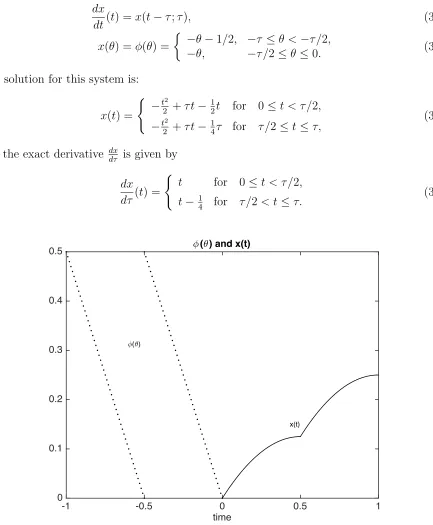
Example 1We consider first an example with a jump discontinuity in the initial data which produces a continuous but not continuously differentiable (with respect to either t or τ) at

t= 1₂.

dx

dt(t) = x(t−τ;τ), (3.3)

x(θ) = φ(θ) =

−θ−1/2, −τ ≤θ <−τ /2,

−θ, −τ /2≤θ≤0. (3.4)

The solution for this system is:

x(t) = (

−t2

2 +τ t− 1

2t for 0≤t < τ /2, −t2

2 +τ t− 1

4τ for τ /2≤t ≤τ,

(3.5)

and the exact derivative dx_dτ is given by

dx dτ(t) =

(

t for 0≤t < τ /2,

t−1

4 for τ /2< t≤τ.

(3.6)

time

-1 -0.5 0 0.5 1

0 0.1 0.2 0.3 0.4

0.5 ?(3) and x(t)

?(3)

x(t)

– For comparing the results, we also compute ∂x_∂τ by solving the sensitivity equations (see description in [5] and references there in). To derive the sensitivity equations, we let

s(t) = ∂x_∂τ(t) and differentiate both sides of equation (3.3) with respect to the delay τ, and obtain the following system of sensitivity equations:

ds

dt(t) = −x˙(t−τ) +s(t−τ), t >0 s(θ) = 0, −τ ≤θ ≤0,

where

˙

x(t−τ) = −1 for t ∈(0, τ /2)∪(τ /2, τ).

The system is not well defined fort ∈[0, τ) ass(τ /2) and ˙x(−τ /2) is not defined. This can be seen from the exact derivative given in equation (3.6) and Figure 2 (right).

– To compute ∂x_∂τ using the complex-step method, first we solve equation (3.3) by re-placing τ with τ +ih for the step size h then we use equation (2.6) and approximate

∂x/∂τ.

The implementation of the complex-step method using either the method of steps or the dde23 Matlab solver does not give the correct solution (see Figure 2 below).

time

0 0.5 1

0 0.5

1 Approximations of dx/d=

sol. of sens. eqns complex-step

time

0 0.5 1

dx/d

=

0 0.25 0.5 0.75

Exact derivative dx/d=

Figure 2: Complex-step approximation of dx/dτ [left] and exact derivativedx/dτ [right] of the solution of DDEs in Example 1 for τ = 1.

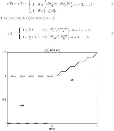
Example 2

In this example we consider a delay system where the history function is a step function with ten jump discontinuities and with the property thatdφ/dθ= 0, θ ∈(−τ,0), producing a continuous but not continuously differentiable solution x(t).

dx

dt(t) =x(t−τ;τ), t∈(0,1] (3.7)

x(θ) =φ(θ) =         

0, θ∈h−2nτ

10 ,

−(2n−1)τ

10

, n= 1, . . . ,5,

1, θ∈h−(2n₁₀−1)τ,−(2n₁₀−2)τ, n = 2, . . . ,5

1, θ∈[−τ

10,0].

, (3.8)

The exact solution for this system is given by

x(t) = 



 1 + n

10τ t∈

h (2n)τ

10 ,

(2n+1)τ

10 i

, n= 0, . . . ,4,

1− n

10τ +t, t ∈ h

(2n−1)τ

10 , (2n)τ

10 i

, n= 1, . . . ,5.

(3.9)

time

-1 0 1

0 0.5 1

1.5 ?(3) and x(t)

?(3)

x(t)

?(3)

x(t)

?(3)

x(t)

The exact derivative is given by

∂x ∂τ(t) =







n

10 t∈

(2n)τ

10 , (2n+1)τ

10

, n= 0, . . . ,4,

−n

10, t∈

_(2n−1)τ 10 ,

(2n)τ

10

, n= 1, . . . ,5.

(3.10)

We implement the complex-step method to approximatedx/dτ as explained in Example 1 with the given step size h= 10−40_.

time

0 0.1 0.2 0.3 0.4 0.5 0.6 0.7 0.8 0.9 -1 -0.8 -0.6 -0.4 -0.2 0 0.2 0.4 0.6 0.8

1 Complex-step approximation of dx/d=

time

0 0.2 0.4 0.6 0.8 1

-0.5 -0.4 -0.3 -0.2 -0.1 0 0.1 0.2 0.3

0.4 Exact derivative dx/d=

Figure 4: Complex-step approximation of dx/dτ [left] and exact derivativedx/dτ [right] of the solution of DDEs in Example 2 for τ = 1.

Here as we can see from Figure 4 (left), the complex-step does not approximate dx/dτ

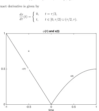
Example 3

In this third example, we consider a system of DDEs where the history function has one removable discontinuity producing a solution with matching right and left hand side derivatives.

dx

dt(t) =x(t−τ;τ), t∈(0, T] (3.11)

x(θ) =φ(θ) = (

3/4, θ=−τ /2

−θ, θ∈[−τ,−τ /2)∪(−τ /2,0]. (3.12)

The exact solution for this problem is given almost everywhere by

x(t) =−t2/2 +τ t, t ∈[0, τ],

and the exact derivative is given by

dx dτ(t) =

(

0, t=τ /2,

t, t∈[0, τ /2)∪(τ /2, τ).

time

-1 -0.5 0 0.5 1

0 0.5

1 ?(3) and x(t)

?(3)

x(t)

Again, letting s(t) = ∂x_∂τ(t), we have the sensitivity system:

ds

dt(t) =−x˙(t−τ) +s(t−τ), t >0, s(θ) = 0, −τ ≤θ ≤0,

where

˙

x(t−τ) =

−1 for 0≤t < τ /2,

−1 for τ /2< t≤τ.

Again, this system is not well defined because s(τ /2) or ˙x(−τ /2) has no value.

time

0 0.5 1

0 0.5

1 Complex-step approximation of dx/d=

time

0 0.5 1

0 0.5

1 ?(3) and x(t)

?(3)

x(t)

Figure 6: Complex-step approximation of dx/dτ [left] and exact derivativedx/dτ [right] of the solution of DDEs in Example 3 for τ = 1.

From Figure 6, we see that the complex-step method approximation of dx_dτ is accurate except at t= τ₂. This is because

lim

h→0−

Im[x(τ /2;τ /2 +ih)]

h = limh→0+

Im[x(τ /2;τ /2 +ih)]

h ,

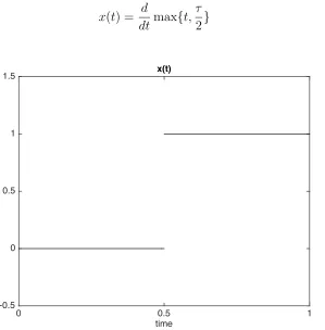
Example 4

In this last example we consider a DDE system with distribution history ‘function’. Here not only the history function lacks smoothness (it is inH−1[−τ,0]), but the solution function

x(t) has a jump at t=τ /2.

dx

dt(t) =x(t−τ;τ), t∈(0, T], (3.13)

x(θ) =φ(θ) = δ(θ+τ /2), θ∈[−τ,0]. (3.14)

The exact solution to this system is given on [0, τ] by

x(t) = d

dtmax{t, τ

2} (3.15)

time

0 0.5 1

-0.5 0 0.5 1

1.5 x(t)

Figure 7: Solution function of Example 4 for τ = 1.

Before computing dx/dτ numerically, we define the Dirac-delta distribution as a limit as follows:

Consider a function b defined by

b(ξ;) = (

0 if |ξ+τ /2|> /2,

Then, the history function takes the form

φ(ξ) =δ(ξ+τ /2) = lim

→0b(ξ;),

that is, for a very small ,

φ(ξ) = δ(ξ+τ /2)≈b(ξ;),

and for our computation, we take= 1·10−10.

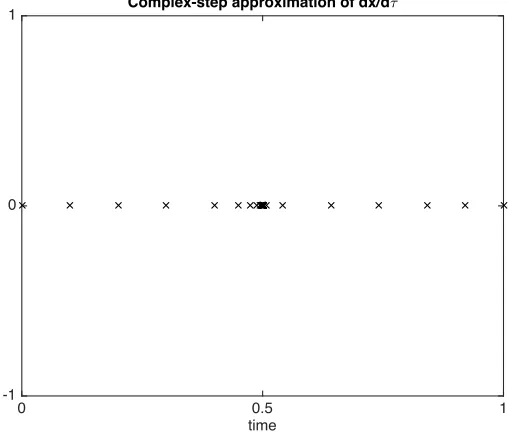
We compute dx/dτ using the complex-step method for t∈[0,1] and τ = 1.

time

0 0.5 1

-1 0

1 Complex-step approximation of dx/d=

Figure 8: Complex-step approximation of dx/dτ of the solution of DDEs in Example 4 for

τ = 1.

Here we see that even though dx/dτ is not defined at t = τ /2, the complex-step imple-mentation provides an accurate approximation of dx/dτ up tot=τ /2 (see Figure 8 above). This is due to the fact that

lim

h→0−

Im[x(·;τ /2 +ih)]

h = limh→0+

Im[x(·;τ /2 +ih)]

4

Conclusions and Further Remarks

We applied the complex-step method to compute sensitivities for delay differential equations with various degree of discontinuities. Our findings show that discontinuities affect the accuracy of the complex-step approximation of the sensitivity when the discontinuities in the history result in corners or jumps in the solution for t > 0. Regardless of the non-smoothness of the initial data, the complex-step implementation using the method of steps and the Matlab solver dde23 provides accurate approximation of the one sided derivatives when they exist and are equal. But we caution especially against the use of dde23 for delay equations with non-smoothness in the initial data. Our computations revealed that cavalier use of dde23 and the complex-step method in this case often produce incorrect results without any warning that the results are in error. In particular see Example 1, Figure 2, where the complex-step method and the dde23 solution of the sensitivity equation for dx_dτ produced incorrect results.

Having observed features of the behavior of the compelx-step method in delay equa-tions, we turned next to a simple ordinary differential in attempts to further understand the complex-step method in the context of simpler systems of the form (1.1) and in particular the simple scalar equation dx_dt = g(t, x;a) = −f(a)x(t) where the parameter a ranges over the values (0,1) and the function f(a) is the quadratic a2. If we consider dx_da ata = 1/2 the complex-step method returns

dx

da(ξ; 1/2) = limh→0−

Im[x(ξ,1/2 +ih)]

h = limh→0+

Im[x(ξ,1/2 +ih)]

h =−2(1/2)ξe

−(1/2)2_ξ

.

In fact this yields the correct results and one can argue this since we have that for any C2

function in q, the 2nd order Taylor expansion

x(t;q+ih) = x(t;q) +ih∂x

∂q(t;q) +R2(h)

where

limR2(h)

h = 0.

If we next consider the example with the same function f(a) except at a= 1/2 wheref

takes on the value f(1/2) = 1/2, we find the limits

lim

h→0−

Im[x(ξ; 1/2 +ih)]

h = limh→0+

Im[x(ξ; 1/2 +ih)]

h =−2(1/2)ξe

−(1/2)2ξ

which are the same results even though dx_da at a = 1/2 does not exist. The corresponding graphs are depicted in Example 5 below which reveal the strengths and weaknesses of using a complex expansion approach to finding sensitivity functions.

Example 5(A Simple Ordinary Differential Equation) We seek a functionx(t) such that

˙

x=−f(a)x(t), a.e.t > 0 (4.1)

where

f(a) = (

a2, a 6= 1/2,

1/2, a= 1/2 .

The solution is given by

x(t;a) =e−a2t (4.3)

so that

˙

x=−f(a)x(t)

almost everywhere int >0, and the exact derivative dx/da is given by

dx

da(t;a) = (−2at)e

−a2_t

, a6= 1/2. (4.4)

a

0.2 0.3 0.4 0.5 0.6 0.7 0.8 0.9 1 0.1

0.2 0.3 0.4 0.5 0.6 0.7 0.8 0.9

1 f(a)

time

0 0.5 1 1.5 2

0.1 0.2 0.3 0.4 0.5 0.6 0.7 0.8 0.9

1 Solution x(t)

time

0 0.5 1 1.5 2

-1.2 -1 -0.8 -0.6 -0.4 -0.2

0 Complex-step approximation of dx/da

Figure 10: Complex-step derivative approximation ofdx/da for example 5 fora = 1/2 (Note that dx/da does not exist at a= 1/2).

time

0 0.5 1 1.5 2

-1.2 -1 -0.8 -0.6 -0.4 -0.2

0 -2(at)exp(-a

2 t) at a=1/2

Figure 11: (−2at)e−a2_t

Acknowledgments

This research was supported in part by the Air Force Office of Scientific Research under grant number AFOSR FA9550-15-1-0298, in part by the National Institute on Alcohol Abuse and Alcoholism under a subcontract from the North Shore Long Island Jewish Health System, Manhasset, NY, and in part by the National Science Foundation under NSF CAREER Award DMS 1555062.

References

[1] W. Kyle Anderson and Eric J. Nielsen, Sensitivity analysis for navier– stokes equations on unstructured meshes using complex variables, AIAA Journal, 39 (2001).

[2] W. Kyle Anderson, Eric J. Nielsen, and D.L. Whitfield, Multidisciplinary sensitivity derivatives using complex variables, Technical report, Engineering Research Center Re-port, Missisipi State University, mSSU-COE-ERC-98-08, July, 1998.

[3] H.T. Banks, Delay systems in biological models: approximation techniques, Nonlinear Systems and Applications(V. Lakshmikantham, ed.), Academic Press, New York, 1977, 21–38.

[4] H.T. Banks, R. Baraldi, K. Cross, K. Flores, C. McChesney, L. Poag, and E. Thorpe, Uncertainty quantification in modeling HIV viral mechanics, CRSC-TR13-16, N. C. State University, Raleigh, NC, December, 2013;Math. Biosciences and Engr.,12(2015), 937–964.

[5] H.T. Banks, K. Bekele-Maxwell, L. Bociu, M. Noorman and K. Tillman, The complex-step method for sensitivity analysis of non-smooth problems arising in biology,Eurasian Journal of Mathematical and Computer Applications ,3 (2015), 16-68.

[6] H.T. Banks and D. M. Bortz, A parameter sensitivity methodology in the context of HIV delay equation models, J. Math. Biol.,50 (2005), 607–625.

[7] H. T. Banks, D. M. Bortz and S. E. Holte, Incorporation of variability into the math-ematical modeling of viral delays in HIV infection dynamics, Math. Biosciences, 183

(2003), 63–91.

[8] H.T. Banks, A. Cintron-Arias, A. Capaldi and A. L. Lloyd, A sensitivity matrix based methodology for inverse problem formulation, CRSC-TR09-09, April, 2009; J. Inverse and Ill-posed Problems, 17 (2009), 545–564.

[10] H.T. Banks, S. Hu, and W.C. Thompson, Modeling and Inverse Problems in the Pres-ence of Uncertainty, Chapman & Hall/CRC Press, Boca Raton, FL, 2014.

[11] H.T. Banks, S. Dediu, and S.E. Ernstberger, Sensitivity functions and their uses in inverse problem, J. Inverse and Ill-posed Problems, 15 (2006), 683—708.

[12] H.T. Banks and Keri L. Rehm, Experimental design for vector output systems, CRSC-TR12-11, N. C. State University, Raleigh, NC, April, 2012; Inverse Problems in Sci. and Engr., 22 (2014) 557–590. doi:10.1080/17415977.2013.797973.

[13] H.T. Banks and K.L. Rehm, Parameter estimation in distributed systems: Optimal design, CRSC TR14-06, N. C. State University, Raleigh, NC, May, 2014; Eurasian Journal of Mathematical and Computer Applications, 2 (2014), 70-79.

[14] H.T. Banks, Danielle Robbins and Karyn L. Sutton, Theoretical foundations for tra-ditional and generalized sensitivity functions for nonlinear delay differential equations CRSC-TR12-14, N. C. State University, Raleigh, NC, July, 2012; Math. Biosci. Engr.,

10 (2013), 1301–1333; http://dx.doi.org/10.3934/mbe.2013.10.1301

[15] H.T. Banks and H.T. Tran, Mathematical and Experimental Modeling of Physical and Biological Processes, CRC Press, Boca Raton, FL, July, 2008, 308pp. published, January 2, 2009.

[16] S.N. Busenberg and K.L. Cooke, eds., Differential Equations and Applications in Ecol-ogy, Epidemics, and Population Problems, Academic Press, New York, 1981.

[17] V. Capasso, E. Grosso and S.L. Paveri-Fontana, eds., Mathematics in Biology and Medicine, Lecture Notes in Biomath., Vol.57, Springer-Verlag, Berlin, Heidelberg, New York, 1985.

[18] J.M. Cushing,Integrodifferential Equations and Delay Models in Population Dynamics, Lec. Notes in Biomath., Vol. 20, Springer-Verlag, Berlin and New York, 1977.

[19] K. P. Hadeler, Delay equations in biology, in Functional differential equations and ap-proximation of fixed points (H. O. Peitgen and H. O. Walther, eds.), Lect. Notes Math.

730 Springer-Verlag Berlin, 1979, 136–156.

[20] G. E. Hutchinson, Circular causal systems in ecology, Annals of the NY Academy of Sciences,50 (1948), 221–246.

[21] G. E. Hutchinson, An Introduction to Population Ecology, Yale University, New Haven, 1978.

[23] J. N. Lyness, Numerical algorithms based on the theory of complex variables, Proc.

ACM 22nd Nat. Conf., 4 (1967), 124—134.

[24] J. N. Lyness and C. B. Moler, Numerical differation of analytic functions, SIAM J. Numer. Anal., 4(1967), 202—210.

[25] Joaquim R. R. A. Martins, Ilan M. Kroo, and Juan J. Alonso. An automated method for sensitivity analysis using complex variables. AIAA Paper 2000-0689 (Jan.), 2000.

[26] Joaquim R. R. A. Martins, Peter Sturdza, and Juan J. Alonso. The complex-step deriva-tive approximation. Journal ACM Transactions on Mathematical Software (TOMS), 2003.

[27] N. Minorsky, Self-excited oscillations in dynamical systems possessing retarded actions, Journal of Applied Mechanics, 9 (1942) A65–A71.

[28] N. Minorsky, On non-linear phenomenon of self-rolling, Proceedings of the National Academy of Sciences, 31 (1945), 346–349.

[29] N. Minorsky, Nonlinear Oscillations, Van Nostrand, New York, 1962.