Cracked beam element formulation for structural analysis
Lucio Nobile(1), Erasmo Viola(1)1) DISTART-Department, Viale Risorgimento 2, 40136 Bologna, Italy ABSTRACT
In this paper, a finite element model for a cracked prismatic beam, under bending moment, axial and shear forces, is developed. The stiffness matrix is derived starting from an integration of stress intensity factors. Translational and rotational mass matrices are the same both for cracked and uncracked Timoshenko beam finite element. The stiffness matrix of the cracked element can be used in any finite element formulation to study static and dynamic behaviour of cracked structures. In the present study the transverse crack has been considered as open.
INTRODUCTION
A crack on a structural member introduces a local flexibility which is a function of the depth of the crack. This flexibility changes the static and dynamic behaviour of the structures.
The fracture mechanics approach can yield the local compliances due to the cracked sections for which expressions for the Stress Intensity Factors (SIFs) can be developed. The local flexibility of the cracked region of the structural element was put into relation with the SIFs. A general method for extending fracture mechanics through the compliance concept to the analysis of a structure containing cracked members was considered in [1]. This paper also shows some examples of the application adopted for the deformation analysis of the cracked specimens. The formulation was also used to study the fatigue evolution of cracked frame-structures and the determination of the bending moment redistribution [2], [3]. At present, the stress intensity factors are theoretically obtained for various types of loading and specimen configurations. The formulas for the SIF as a function of the crack depth can be found in several handbooks [4]. Remarkably two simple methods for close approximation of stress intensity factors in cracked or notched beams were proposed [5], [6].
One was based on elementary beam theory estimation of strain energy release rate as the crack is widened into a fracture band, the other was based on elementary beam theory equilibrium condition for internal forces evaluated in the cross section passing through the crack tip. In this paper, the stiffness matrix for a two-node cracked Timoshenko beam element is derived. The equation of motion of the complete system in a fixed co-ordinate system includes translational and rotatory mass matrices. A parametric study of a transverse open crack has been carried out for various crack depths and crack locations. It also determines the changes in eigenfrequencies with two different beam models.
STIFFNESS MATRIX OF CRACKED ELEMENT
For general loading, a local stiffness matrix relates forces to displacements. In this analysis, rotational and translational crack compliance are assumed in the local flexibility matrix. So bending, shear and axial effects will be included.
According to Okamura et al. [1], cracked member can be separated at the cracked section and both portions may be connected by a spring with spring constant Db, Ds, Da, corresponding to bending moment M, shear force T and axial force P, respectively. For general plane loading the strain energy of a beam element without a crack, is
W
EI M L MTL
T L P L
EA
T L G
( )0 1 2 2 2 3 2 2
2 3
1 2
1 2
= − +
+ + Λ (1)
where E is the Young's modulus, G is the shear modulus, L the length of the beam element, A being the area of the cross-section and Λ = A/χ a coefficient which depends on the shear coefficient χ.
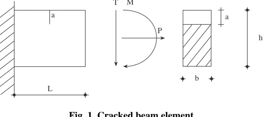
The additional strain energy due to the crack, as in fig. 1, is:
W( )1 b a K2I K2II E ( )KIII2 E da
0 1
=
∫
(
+)
′ + +ν (2)where E′ = E/(1 – ν2) for plane strain, E′ = E for plane stress, ν is the Poissons' ratio and KI, KII, KIII are the crack tip stress intensity factors for opening mode, sliding mode and tearing mode of crack surface displacements, respectively. It should be noted that the K values are linear factors containing the load linearly. The superposition of these three modes is sufficient to describe the most general 3-dimensional case of local crack-tip deformation and stress fields.
SMiRT 16, Washington DC, August 2001 Paper # 1840
Since the cracked element is subject to three loading force systems applied simultaneously as shown in fig. 1, the total K is the algebraic sum of K values for each system applied separately. However, since different fields of stress occur for each mode, then the sums must be separated for each mode.
L a
T M
P
a
b
h
Fig. 1. Cracked beam element.
By considering the actions of bending moment M, shear force T and axial force P simultaneously, equation (2) becomes
W b KIM KIT KIP KIIT E da a
( )1 2 2
0
=
(
+ +)
+( )
′
∫
(3)where stress intensity factors are given by [4]
KIM=σM π σ πa FIM , KIT = T a FIT , KIP =σ π τP a FIP , KIIT = πa FII (4) with
FIM =FIT =FI = sin
+
[
−]
( ) ( / ) tan( / ) . . ( / ) cos( / )
ξ π π ξ ξ πξ
πξ
2 2 0 923 0 199 1 2
2
4
(5)
FIP( ) ( / ) tan( / ) sin
. . . ( / )
cos( / )
ξ π π ξ ξ ξ π ξ
πξ
= 2 2 0 752+2 02 +0 37 1
[
− 2]
23
(6)
FII =FII = −
− + +
−
( )ξ ( ξ ξ ) . . ξ . ξ . ξ
ξ
3 2 1 122 0 561 0 085 0 18 1
2
2 3
(7)
where ξ = a/h.
Stresses σM, σT, σP, τ can be expressed as
σM σT σP τ
M
bh
P bh
T bh
= 6 2 , =3TL = =
bh2 , ,
(8)
By substituting Eqs. (4)-(8) into Eq. (3) and assuming
RI aF daI R aF da Q aF da F da a
II II
a
IP a
IP a
=
∫
2 =∫
=∫
∫
0
2 0
2
0 0
, , , Z = aFI (9)
n
E bh
=
′ ′
36 4
π π
, m = E bh2
(10)
the strain energy due to the crack gets the form
W n M TL R mP Q m
h MP TPL Z mT R
c I II
( )
( / ) ( )
1 2 2 2
2 6 2
The flexibility matrices of cracked and uncracked element with constraints (fig. 1) may be calculated by means of Castigliano's theorem:
cij=∂ W ∂ ∂F Fi j = 2
1 2 3
/ (i, j , , ) (12)
where F1 = P, F2 = T, F3 = M and W = W(0) or W = W(1). For cracked element W = W(1) and the flexibility matrix has the form
c
mQ mZL
h
mZ h mZL
h
nR L
mR nR L
mZ
h nR L nR
I
II I
I I
( )1 2
2 6 12
6
2 2
12
2
= +
(13)
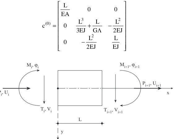
In the case of uncracked element W = W(0) and the 3 × 3 flexibility matrix is
c
L EA
L EJ
L G
L EJ L
EJ
L EJ
( )0 3 2
2
0 0
0
3 2
0
2
= + −
−
Λ (14)
L y
Pi+1, Ui+1 x Mi+1, ϕi+1
Ti+1, Vi+1 Pi, Ui
Mi, ϕi
Ti, Vi
Fig. 2. Typical element with nodal displacements and nodal forces.
Nodal forces on typical element must satisfy the equilibrium condition (see fig. 2), that can be written in the extended matrix form
P
T
M
P
T
M
L
P i
i
i
i
i
i
i
+
+
+
+
=
−
−
− −
1
1
1
1 0 0
0 1 0
0 1
1 0 0
0 1 0
0 0 1
1 1
1
1 T
M i
i +
+
Denoting by
AT= L
−
− −
−
1 0 0 1 0 0
0 1 0 1 0
0 0 1 0 0 1
(16)
the stiffness matrix for the cracked element may be derived as:
k A c c A
c=
(
( )0 + ( )1)
−1 T(17) in which the notation is obvious.
Introducing Eqs. (13), (14), (16) into Eq. (17) we obtain the cracked element stiffness matrix expressed in the extended form
kc
c c c c
c c c c
c c c c c c
c c c c
c c c c
c c c c c c
k k k k
k k k k
k k k k k k
k k k k
k k k k
k k k k k k
=
11 13 14 16
22 23 25 26
31 32 33 34 35 36
41 43 44 46
52 53 55 56
61 62 63 64 65 66
0 0
0 0
0 0
0 0
(18)
which has the entries
k k k k EA L LR d
L
c c c c I
11 14 41 44 2
6
1
= − = − = = +
+
( )
( Ω)
(19)
k k k k k k k k EA Z
L
c c c c c c c c
13 16 31 34 43 46 61 64 2
1
= − = = − = − = = − = = −
+ π
( Ω)
(20)
k k k k EJ
L hR
c c c c
II
22 25 52 55 3
12
1 2
= − = − = =
+ +
( Γ) π
(21)
k k k k k k k k EJL
L hR
c c c c c c c c
II
23 26 32 35 53 56 62 65 3
6
1 2
= = = − = − = − = = − = −
+ +
( Γ) π
(22)
k k
EJL Qd Qd R d QR d d Z hR
L
QR
L
L hR
c c
I I
II II
II 33 66
2 2 2 2
3
2
4
3
4 1 2 8 18 36 36 2 4
1 2 1
= =
+ + + + + − + +
+ +
[
]
+Γ
Γ Ω
( )
( ) ( )
π π
π (23)
k k
EJL Qd Qd R d QR d d Z hR
L
QR
L
L hR
c c
I I II II
II 36 63
2 2 2 2
3
2
4
3
2 1 2 4 18 36 36 2 4
1 2 1
= =
− + + + + − + −
+ +
[
]
+Γ
Γ Ω
( )
( ) ( )
π π
where
d
hL d QR dI d Z
= π , = 12EJ ,
(
+ −)
G L
= 2Qd + 6R
2 I
Γ
Λ Ω 12 12
2 2 2
(25)
It should be noted that the uncracked element stiffness matrix may be deduced from Eqs. (18)-(25). The stiffness matrix for Thimoshenko beam element will be derived by neglecting the terms Z, Q, RI, RII. Moreover, by setting Γ = 0 in resultant equations, the above coefficients (18)-(24) reduce to elements of the Euler-Bernoulli beam model.
MASS MATRIX
The consistent translational mu and mν and rotational mϑ mass matrices are assumed the same both for cracked and uncracked Timoshenko beam finite element. The above matrices can be expressed in the well known forms [7] and [8]. The total mass matrix of the two mode finite element is
m=mu+mν+mϑ (26)
The above mass matrices can be derived by using the Kinetic energy of the beam element of length L
τ µ ∂ ∂ µ ∂ ∂ µ ∂θ∂ = + +
∫
∫
∫
1 2 1 2 1 2 0 2 0 2 0 2 A ut dx A
v
t dx J t dx
L L L
(27)
including the effects of both translational displacements u, ν and rotatory inertia, respectively. In (27) µ is the mass density of the material. For a finite element formulation, the displacements u, ν and the rotation ϑ can be expressed as
u N N N N N N
N N N N N N
N N N N N N u
u u u u u u
ν ϑ ν ϑ ν ϑ ν ν ν ν ν ν ϑ ϑ ϑ ϑ ϑ ϑ =
1 2 3 4 5 6
1 2 3 4 5 6
1 2 3 4 5 6
1 1 2 2 2 u1 (28)
where Nui, Nνi, Nϑi (i = 1, 2, …, 6) are the interpolation functions for axial displacement, transverse displacement and for the rotation of the cross-section about the positive z axis. So, the displacement field u = u(x), ν = ν (x), ϑ = ϑ (x) in the beam element is linearly interpolated by relation (28), where u1, ν1, ϑ1, u2, ν2, ϑ2 is the set of degrees of freedom for a two node beam element. It should be noted that in vibration displacement field functions u, ν, ϑ and nodal displacements u1, ν1, ϑ1, u2,
ν2, ϑ2 are all time-depending. However, for the purpose of deriving stiffness and mass matrices, they can all be regarded as constant in time. The resulting explicit form of shape functions for axial displacement u are:
N x
L
x
L N N N
u1= −1 , Nu4 = , Nu2 = u3= u5= u6 =0 (29) for displacement ν in the y direction, are
N N x
L x L x L L x L x L x L ν ν ν ν 1 4 3 2 3 2 0 1
1 2 3 1
1 2 2 1 2
= = = + − − + + = − + − + + + , ( ) ( ) N N 2 3 Γ Γ Γ Γ Γ Γ = + − − = − + − − −
2 3 2
3 2
1
1 2 3
1 1 2 2
, N
and for bending rotation may be written as: N N L x L x L x L x L L x L θ θ θ θ θ 1 4 2 2 0 6 1 1
1 3 4 1
6 1 = = = − + − = + − + + + = + + , ( ) ( ) ( ) ( ) ( ) N
N , N
2 3 5 Γ Γ Γ Γ Γ 2 2 2 1
1 3 2
− = + − − x L x L x L Nθ6
( Γ) ( Γ)
(31)
The above shape functions are determined so that they exactly satisfy the homogeneous form of the static equations of equilibrium of a uniform Timoshenko beam axially loaded [7][8]:
d dx EA du dx G d dx d dx EJ d dx G d dx = + = − + + =
0, d 0, 0
dx Λ ν θ Λ
θ ν θ
(32)
The explicit expressions for the elements of translational mass matrices mu and mν and for the rotational mass matrix mϑ are given as:
mij N AN dx N AN dx N JN dx
u ui uj L i j L i j L =
∫
µ ν =∫
µ =∫
µ ν ν θ θ θ , ,0 mij 0 mij 0 (33)
respectively, for i, j = 1, 2,… 6. The mass matrices constructed in this way are said to be consistent in the sense that they are obtained for the same displacement approximation as the stiffness matrix. Letting
mt =mu +mν (34)
where mt is the total translational mass matrix, Eq. (26) yields
m=mt+mϑ (35)
By substituting (29)-(31) into (33) and carrying out the integration over the beam-length L, the following mass matrices will be derived
mt AL
L L L = + + + + + + + + + − + + + + + + µ ( ) ( ) ( ) 1 1
3 0 0
1
6 0 0
13 35 7 10 3 11 210 11
120 24 0
9 70 3 10 6 13 420 3 40 24
105 60 120 0
13 210 3 40 24 2 2 2
2 2 2 2
2 2 2 Γ Γ Γ Γ Γ Γ Γ Γ Γ Γ Γ Γ Γ Γ Γ 1 − + + + + + − + + + + 1
140 60 120 1
3 0 0
13 35 7 10 3 11 210 11 120 24 1
mϑ= µ
+
−
− −
+ +
− − − + −
− −
J
L
L L
L L L
SIMM L
( )
. 1
0 0 0 0 0 0
6 5
1
10 2 0
6 5
1 10 2
2
15 6 3 0
1 10 2
1
30 6 6
0 0 0
6 5
1 10 2 2
2
2 2 2
Γ
Γ Γ
Γ Γ Γ Γ Γ
Γ
2 2
15 6 3 2
2
+ +
Γ Γ
L
(37)
The above mass matrices depend upon Γ and both these matrices reduce to the Bernoulli-Euler form by setting Γ = 0. NUMERICAL RESULTS
The equations of motion for the complete system in a fixed co-ordinate system may be derived by using the standard finite element method to the fixed-hinged plane frame represented in fig. 3
Mx.. + Kx = p (38)
where M is the mass matrix of the assembled system, K the structural stiffness matrix and
x=
[
u ui i i un n n]
T
1 1 1ν ϑ,K, ν ϑ,K, ν ϑ (39)
is the generalized displacement vector and
p=
[
P T M P T Mi i i P T Mn n n]
T
1 1 1,K, ,K, (40)
is the external excitation vector. In numerical calculations, the crack is set only in one finite element of the discretized cracked structure.
a
5 cm
h = 10 cm
1 2
3
4 B = 40 cm
H = 80 cm
Cracked section
Fig. 3. Cracked fixed-hinged frame.
The problem of determining the natural vibration frequencies and the associated mode shapes of a system always leads to solving the eigenproblem of the homogeneous linear system
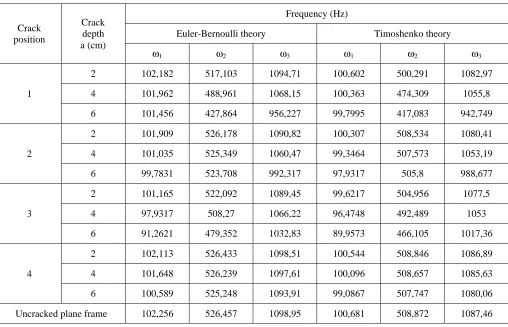
where the mass and stiffness matrices are nearly always symmetric and positive definite. In the present work, four crack position are fixed, as shown in fig. 3 by 1, 2, 3, 4. For each position, three crack depths are considered. Frequencies ω1, ω2,
ω3 for cracked and uncracked plane frame are shown in table 1, both Euler-Bernoulli theory and Timoshenko theory, for various crack depth and crack position, and assuming E = 2.06 ⋅ 105 N/mm2, µ = 7750 kg/m3.
Table 1. Frequencies for cracked and uncracked plane frame.
Frequency (Hz)
Euler-Bernoulli theory Timoshenko theory
Crack position
Crack depth a (cm)
ω1 ω2 ω3 ω1 ω2 ω3
2 102,182 517,103 1094,71 100,602 500,291 1082,97
4 101,962 488,961 1068,15 100,363 474,309 1055,8
1
6 101,456 427,864 956,227 99,7995 417,083 942,749
2 101,909 526,178 1090,82 100,307 508,534 1080,41
4 101,035 525,349 1060,47 99,3464 507,573 1053,19
2
6 99,7831 523,708 992,317 97,9317 505,8 988,677
2 101,165 522,092 1089,45 99,6217 504,956 1077,5
4 97,9317 508,27 1066,22 96,4748 492,489 1053
3
6 91,2621 479,352 1032,83 89,9573 466,105 1017,36
2 102,113 526,433 1098,51 100,544 508,846 1086,89
4 101,648 526,239 1097,61 100,096 508,657 1085,63
4
6 100,589 525,248 1093,91 99,0867 507,747 1080,06
Uncracked plane frame 102,256 526,457 1098,95 100,681 508,872 1087,46
REFERENCES
1. Okamura, H., Watanabe, K. and Takano, H., Applications of the compliance concept in fracture mechanics, ASTM, STP 536, 1973, pp. 423-438.
2 . Carpinteri, A., Di Tommaso, A. and Viola, E., “Fatigue evolution of multicracked frame structures”, Proceedings International Conference Anal. Exp. Fracture Mechanics, Edited by G.C. Sih, Rome, 1980, pp. 417-430,.
3. Viola, E. and Pascale G., “Static fatigue and fracture analysis of cracked beams on elastic foundation”, Engineering Fracture Mechanics, Vol. 21(2) , 1985, pp. 365-375.
4. Tada, H., Paris, P.C. and Irwin, G.R., The stress analysis of cracks Handbook, Del Research Corporation, Hellertown, 1973.
5. Kienzler, R. and Herrmann, G., “An elementary theory of defective beams”, Acta Mechanica, Vol. 62, 1986, pp. 37-46. 6. Nobile, L., “Mixed mode crack initiation and direction in beams with edge crack”, Theoretical and Applied Fracture
Mechanics, Vol. 33, 2000, pp. 107-116.
7. Kosmata, J.B., “An improved two-node finite element for stability and natural frequencies of axial loaded Timoshenko beams”, Computers and Structures, Vol. 57(1), 1995, pp. 141-149.