MAZZARO, GREGORY J. Time-Frequency Effects in Wireless Communication Systems. (Under the direction of Professor Michael B. Steer).
by
Gregory James Mazzaro
A dissertation submitted to the Graduate Faculty of North Carolina State University
in partial fullfillment of the requirements for the Degree of
Doctor of Philosophy
Electrical Engineering
Raleigh, NC
2009
APPROVED BY:
Dr. Michael B. Steer Dr. Kevin G. Gard Chair of Advisory Committee
Dr. J. Keith Townsend Dr. Mohammed A. Zikry
BIOGRAPHY
Gregory James Mazzaro was born in Bronxville, New York. He received his B.S. degree in Electrical Engineering from Boston University in 2004 and his M.S. degree in Electrical Engineering from The State University of New York at Binghamton in 2006. Since 2006, he has worked toward the Ph.D. degree as a research assistant for the Electronics Research Laboratory at North Carolina State University.
ACKNOWLEDGMENTS
I would like to thank several people for their support during my completion of this dis-sertation: Dr. Michael Steer, for guiding me through my publications & presentations, for providing me with professional contacts to the Army Research Laboratory, and for remind-ing me of the broader impact of my work; Dr. Kevin Gard, for helpremind-ing me to take relevant and accurate data, for answering my many lab-related questions, and for staying in touch while on sabbatical from NC State; Dr. Keith Townsend and Dr. Mohammed Zikry, for serving on my Ph.D. advisory committee; Dr. Dev. Palmer, for serving as a technical con-sultant and last-minute addition to the committee; Dr. Aaron Walker, for teaching me to use much of the test equipment in the Electronics Research Laboratory; and Dr. Frank Hart for bringing me up-to-speed using fREEDA and LaTeX.
I would also like to thank my graduate student colleagues and friends for their critical thinking, their entrepreneurial spirit, and their senses of humor: Jon Wilkerson, Glen Garner, Rob Harris, Chris Saunders, Chris Mineo, Austin Samples, Samson Melamed, Vrinda Haridasan, Justin Lowry, Jie Hu, Eric Phillips, Nikhil Kriplani, and Zhiping Feng. These people provided me with an enjoyable working environment for many months. Their wisdom and creativity have been invaluable to me, both professionally and personally.
TABLE OF CONTENTS
LIST OF FIGURES . . . ix
LIST OF TABLES . . . xiv
1 Introduction . . . 1
1.1 Overview . . . 1
1.2 Motivations . . . 2
1.2.1 When to Use Time-Domain and Time-Frequency Analysis . . . 4
1.2.2 Objective: Explain, Model, & Apply Time-Frequency Effects . . . . 5
1.3 Original Contributions . . . 5
1.3.1 Evaluation of Filter Transients on Frequency-Hopping . . . 5
1.3.2 Pulse Decay Methods for Estimating Filter Parameters . . . 6
1.3.3 Lowpass-Prototyped Filter Transient Response Solution . . . 6
1.3.4 Method for Measuring IM Distortion by Switched Tones . . . 6
1.3.5 One-Port Nonlinear Method for Filter Passband Extraction . . . 7
1.3.6 Transmission-Line Separation of Coupled Resonators . . . 7
1.3.7 Linear Amplification by Time-Multiplexed Spectrum (LITMUS) . . 7
1.4 Dissertation Outline . . . 8
1.5 Published Works . . . 9
1.5.1 Journal papers . . . 9
1.5.2 Conference papers . . . 9
1.6 Unpublished Works . . . 10
2 Time-Frequency Concepts and Prior Research . . . 11
2.1 Introduction . . . 11
2.2 Important Quantities and their Regions of Applicability . . . 12
2.2.1 Frequency: Fourier vs. Instantaneous . . . 12
2.2.2 Linear Delay: Group vs. Average . . . 14
2.2.3 Quality Factor: Fractional Bandwidth vs. Energy Decay . . . 19
2.2.4 Summary . . . 20
2.3 Review of Analysis Techniques . . . 20
2.3.1 Short-Time Fourier Transform . . . 21
2.3.2 Wavelet Transform . . . 24
2.3.3 Lowpass Prototyping . . . 27
2.3.4 Summary . . . 29
2.4 Transients in Linear Narrowband Systems . . . 29
2.4.1 Discovery of Transients, Quasi-Stationary Behavior . . . 29
2.4.3 Laplace Methods . . . 33
2.4.4 Summary & Current Research . . . 35
2.5 Extraction of Resonant Circuit Parameters . . . 35
2.5.1 Single-Resonator Assumption . . . 36
2.5.2 Steady-State Methods . . . 36
2.5.3 Time-Frequency Methods . . . 40
2.5.4 Summary & Current Research . . . 41
2.6 Nonlinearities in Narrowband Circuits . . . 41
2.6.1 Intermodulation Distortion and Filtering . . . 42
2.6.2 Current Research . . . 42
2.7 Linear Multi-Tone Signal Amplification . . . 43
2.7.1 High-Power Linear AM Transmission . . . 43
2.7.2 Current Research . . . 44
2.8 Summary & Conclusions . . . 44
3 Linear Transient Distortion in Narrowband Systems . . . 46
3.1 Introduction . . . 46
3.2 Bandpass Response to Single-Tone Pulses . . . 47
3.2.1 Simulation . . . 47
3.2.2 Measurements . . . 50
3.2.3 Discussion: Resonator Cascade . . . 53
3.2.4 Transient Resonator Interactions . . . 55
3.2.5 Summary . . . 61
3.3 Bandpass Response to Switched-Tone Signals . . . 63
3.3.1 Switched-Tone Transmission Simulation . . . 63
3.3.2 Switched-Tone Transmission Measurements . . . 66
3.3.3 Pulse Overlap & Two-Tone Interference . . . 67
3.3.4 Pulsed & Switched Reflection Simulations . . . 67
3.3.5 Wireless Switched-Tone Reflection Measurements . . . 71
3.3.6 Summary . . . 73
3.4 Mathematical Modeling of Filter Transients . . . 73
3.4.1 Prior Approaches . . . 73
3.4.2 Response Derived from Lowpass Prototyping . . . 74
3.4.3 Summary . . . 76
3.5 Case-Study: Frequency-Hopped Communications . . . 77
3.5.1 Settling Time vs. Group Delay . . . 77
3.5.2 Impact of Filtering on Signal-to-Noise Ratio . . . 79
3.5.3 Summary . . . 81
3.6 Conclusions . . . 82
4 Linear Metrology of Bandpass RF Components . . . 84
4.1 Introduction . . . 84
4.2 Extraction of Resonator Q from RF Pulse Decay . . . 85
4.2.2 Equivalence of Quality Factor in Time & Frequency Domains . . . . 88
4.2.3 Measurements . . . 93
4.2.4 Discussion: Coupled Resonators . . . 94
4.2.5 Summary . . . 95
4.3 Estimation of Filter Bandwidth from RF Pulse Response . . . 96
4.3.1 Circuit Bandwidth & Rippling in its Pulse Response . . . 96
4.3.2 Simulation . . . 98
4.3.3 Measurements . . . 99
4.3.4 Summary . . . 101
4.4 Extraction of S-Parameters from Short-Pulse Responses . . . 101
4.4.1 Narrow Pulses, Wideband Spectra . . . 103
4.4.2 Simulation . . . 104
4.4.3 Measurement . . . 106
4.4.4 Summary . . . 110
4.5 Conclusions . . . 110
5 Nonlinear Metrology of Bandpass RF Systems . . . 112
5.1 Introduction . . . 112
5.2 Generation of Multisines from Switched Tones . . . 114
5.2.1 Switched-Tone to Steady-Tone Theory . . . 114
5.2.2 Measurements . . . 116
5.2.3 Mechanism for Conversion: Filter Energy Storage . . . 116
5.2.4 IP3 Measurement by Switched Tones . . . 120
5.2.5 Summary . . . 122
5.3 One-Port Filter Passband Extraction . . . 123
5.3.1 Transfer Function Magnitude from IM Products . . . 123
5.3.2 Wireline Measurement . . . 125
5.3.3 Wireless Measurement . . . 127
5.3.4 Summary . . . 130
5.4 IM Distortion in Frequency-Hopping Systems . . . 130
5.4.1 Origin of IMD in Frequency-Hopping . . . 130
5.4.2 Measurements . . . 131
5.4.3 Summary . . . 132
5.5 Conclusions . . . 133
6 Linear Amplification by Time-Multiplexed Spectrum. . . 135
6.1 Introduction . . . 135
6.2 Distortion Reduction Theory . . . 136
6.2.1 Time-Multiplexed Sinusoids . . . 136
6.2.2 Intermodulation Cancellation . . . 139
6.2.3 Summary . . . 145
6.3 Experimental Validation . . . 145
6.3.1 Narrowband Measurements, 2 Tones . . . 145
6.3.3 Wideband Measurements, 6+ Tones . . . 149
6.3.4 Summary . . . 153
6.4 Linear Signal Recovery . . . 153
6.4.1 Theory . . . 153
6.4.2 Measurement . . . 154
6.4.3 Summary . . . 158
6.5 Conclusions . . . 159
7 Conclusions and Future Work. . . 160
7.1 Summary of Research and Original Contributions . . . 160
7.2 Future Research . . . 162
Bibliography . . . 163
Appendices . . . 169
A Instrument Control & Calibration . . . 170
A.1 USB to GPIB Drivers . . . 170
A.2 Agilent E8267C Signal Generator . . . 172
A.2.1 Single-Tone Pulses . . . 172
A.2.2 Switched-Tone Pulses . . . 175
A.2.3 100 MS/s Time-Multiplexed Multi-Tones . . . 178
A.3 Tektronix TDS684B Oscilloscope . . . 181
A.4 Agilent E4445A Spectrum Analyzer . . . 184
A.5 Agilent N6030A Wideband Signal Generator . . . 186
A.6 Agilent N5230A Vector Network Analyzer . . . 192
A.6.1 Two-Port Calibration . . . 192
A.6.2 Viewing & Saving S-Parameters . . . 193
A.6.3 Viewing & Saving Group Delay . . . 194
B fREEDA Elements . . . 195
B.1 vlfmpulse — Linear FM Voltage Source . . . 195
B.2 chebyshevbpf — Lumped Chebyshev Bandpass Filter . . . 196
C Matlab Helper Functions . . . 198
C.1 RF Envelope Extraction . . . 198
C.2 Generalized Fourier Transform . . . 199
C.3 Bandpass Element Values from Low-Pass Prototypes . . . 200
C.4 One-Sided Fourier Transform . . . 202
C.5 Ideal Bandpass Filter . . . 203
D Cauer 1 vs. Cauer 2 Filter Designs . . . 204
D.1 One Transfer Function, Two Reflection Coefficients . . . 204
E Filters Used in This Study . . . 209
E.1 Filter Parameters from Manufacturer Datasheets . . . 209
E.1.1 900-MHz Chebyshev Filters from Trilithic . . . 209
E.1.2 465-MHz Chebyshev Filters from Trilithic . . . 210
E.1.3 4th-Order Chebyshev Filters from Trilithic . . . 210
E.1.4 5th-Order Chebyshev Filters from K&L Microwave . . . 211
E.2 S-Parameters from the Agilent N5230A . . . 212
E.2.1 Magnitude & Phase . . . 212
LIST OF FIGURES
Figure 2.1 Linear chirp example: time-domain signal . . . 15
Figure 2.2 Linear chirp: Fourier vs. Instantaneous frequency. . . 15
Figure 2.3 Group delay example: 5th-order 1% Chebyshev filter . . . 16
Figure 2.4 Spectrum of a pulsed RF signal. . . 17
Figure 2.5 Short-Time Fourier Transform example, overlapping pulses . . . 22
Figure 2.6 STFT of overlapped pulses without windowing . . . 22
Figure 2.7 STFT of overlapped pulses with sliding rectangular window . . . 23
Figure 2.8 Morlet wavelet example . . . 25
Figure 2.9 Linear chirp in Gaussian white noise. . . 25
Figure 2.10 Chirp signal extracted from noise using wavelets . . . 26
Figure 2.11 Lowpass equivalent circuit for 5th-order Chebyshev filter . . . 27
Figure 2.12 Quasi-stationary vs. non-quasi-stationary filter responses . . . 31
Figure 2.13 Single-resonator filter circuit simplification. . . 36
Figure 2.14 Augmented single-resonator circuit . . . 38
Figure 2.15 The Critical-Points method. . . 39
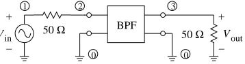
Figure 3.1 Filter pulse transmission test schematic. . . 48
Figure 3.2 Collection of simulated filter pulse transmission responses . . . 49
Figure 3.3 Single-frequency pulse generated by the Agilent E8267C . . . 51
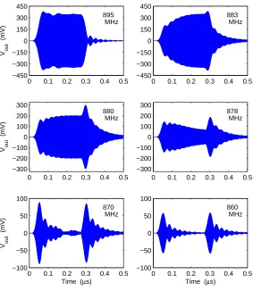
Figure 3.4 Measured pulse transmissions, 900-MHz 4% filter, frequency varied . . . 52
Figure 3.6 Simulated pulse transmission, 7th-order 3% Chebyshev filter . . . 55
Figure 3.7 Resonator-separation simulation schematic . . . 56
Figure 3.8 Simulated RF pulse applied to bandpass filters . . . 58
Figure 3.9 Resonator-separation simulation, different ports, same pulse . . . 58
Figure 3.10 Resonator-separation simulation, output port, multiple pulse arrivals . . . 59
Figure 3.11 Partial sums of pulse arrivals vs. complete pulse transmission . . . 60
Figure 3.12 RMS difference of partial sums from total pulse transmission . . . 61
Figure 3.13 Resonator-separation result, pulse frequency varied . . . 62
Figure 3.14 Collection of simulated switched-tone filter transmission responses . . . 64
Figure 3.15 Measured switched transmissions, 900-MHz 4% filter, frequency varied . . 66
Figure 3.16 Filter reflection test schematic . . . 68
Figure 3.17 Collection of simulated filter transient reflection responses . . . 70
Figure 3.18 Wireless switched-tone reflection measurement system . . . 72
Figure 3.19 Wireless switched-tone measurement results . . . 72
Figure 3.20 Lowpass prototype circuit, 7th-order Chebyshev filter . . . 74
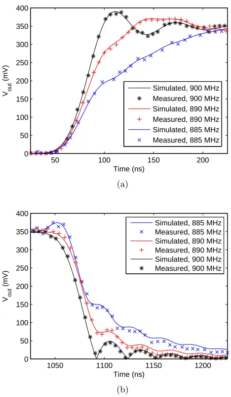
Figure 3.21 Measured filter output vs. lowpass-prototype-derived response . . . 77
Figure 3.22 Settling time vs. group delay for simulated 7th-order 4% filter . . . 78
Figure 3.23 Pulse overlap caused by filtering communications pulses . . . 80
Figure 3.24 Signal degradation caused by pulse overlap between two users . . . 81
Figure 4.1 Filter pulse decay test schematic . . . 86
Figure 4.2 Simulated filter pulse envelope decay, 7th-order 900-MHz filters . . . 87
Figure 4.3 Lowpass-equivalent circuit of 7th-order Chebyshev filter . . . 90
Figure 4.4 Bandpass transient response vs. lowpass prototype transient response. . . 90
Figure 4.6 Filter decay response measurement system. . . 93
Figure 4.7 Measured filter decay envelopes, 7th-order 900-MHz designs . . . 94
Figure 4.8 Filter bandwidth extraction circuit . . . 99
Figure 4.9 Simulated turn-on response and time derivative, 7th-order 4% filter . . . 100
Figure 4.10 Measured decay response and RF envelope, 900-MHz 3% filter . . . 102
Figure 4.11 Linear passband extraction circuit . . . 102
Figure 4.12 Simulated short-pulse waveform and spectrum . . . 104
Figure 4.13 Simulated short-pulse transmission and spectrum, 5th-order 1% filter . . . 106
Figure 4.14 Simulated short-pulse reflection and spectrum, 5th-order 1% filter . . . 107
Figure 4.15 Time-domain vs. frequency-domain S-parameters, simulated . . . 108
Figure 4.16 Linear passband extraction measurement system. . . 108
Figure 4.17 Measured short-pulse transmission and reflection, 465-MHz 1% filter . . . . 109
Figure 5.1 Two-tone switched-to-multisine conversion schematic . . . 115
Figure 5.2 Switched-to-multisine conversion hardware. . . 117
Figure 5.3 Measured time-domain traces, 2 switched tones to a 2-tone multisine . . . 117
Figure 5.4 Fast-switching filter response simulation circuit . . . 118
Figure 5.5 Simulated fast-switched response, 7th-order 465-MHz 3% filter . . . 119
Figure 5.6 Output IP3 measurement for Ophir 5162 using switched tones . . . 121
Figure 5.7 Switched-tone IP3 measurement system . . . 122
Figure 5.8 Nonlinear passband extraction circuit. . . 124
Figure 5.9 Nonlinear passband extraction measurement system . . . 126
Figure 5.10 Alternate nonlinear passband extraction system . . . 126
Figure 5.11 Passband extraction measurements, 7th-order 900-MHz filters . . . 128
Figure 5.13 Wireless switched-tone nonlinear measurement results . . . 129
Figure 5.14 Frequency-hopping IMD measurement system . . . 132
Figure 5.15 Measured IMD produced by single switch/filter/amplify event . . . 133
Figure 6.1 LITMUS circuit architecture . . . 137
Figure 6.2 Switched-tone spectrum, 10 tones . . . 137
Figure 6.3 Distortion reduction measurement setup, 2 tones . . . 146
Figure 6.4 Measured IM3 for the RF2320 amplifier with time-multiplexing . . . 148
Figure 6.5 Random-phase distortion reduction measurement setup . . . 149
Figure 6.6 Measured distortion, with LITMUS vs. without, random phases . . . 150
Figure 6.7 Wideband distortion reduction measurement setup . . . 151
Figure 6.8 Measured distortion, time-multiplexed vs. non-multiplexed, 20 tones . . . . 152
Figure 6.9 Linear recovery measurement setup . . . 155
Figure 6.10 Measured time-domain linear recovery . . . 156
Figure 6.11 Measured frequency-domain linear recovery . . . 157
Figure 6.12 Measured distortion, multiplexed vs. non-, filtered, 4 tones . . . 158
Figure B.1 VLFMpulse element . . . 195
Figure B.2 ChebyshevBPF circuit. . . 196
Figure C.1 Lowpass prototype vs. bandpass circuit. . . 200
Figure D.1 Lowpass prototypes vs. bandpass circuits, 3rd-order filters . . . 206
Figure D.2 Cauer 1 vs. Cauer 2 simulation circuit . . . 206
Figure D.3 Cauer 1 vs. Cauer 2 architecture, steady-state response comparison . . . 207
Figure E.1 Trilithic 7BC900/27-3-KK S-parameters . . . 212
Figure E.2 Trilithic 7BC900/36-3-KK S-parameters . . . 213
Figure E.3 Trilithic 7BC900/45-3-KK S-parameters . . . 214
Figure E.4 Trilithic 7BC465/5-3-KK S-parameters . . . 215
Figure E.5 Trilithic 5BC465/5-3-KK S-parameters . . . 216
Figure E.6 Trilithic 4BC500/20-3-KK S-parameters . . . 217
Figure E.7 Trilithic 4BC1000/40-3-KK S-parameters . . . 218
Figure E.8 Trilithic 4BC2000/80-3-KK S-parameters . . . 219
Figure E.9 K&L Microwave 5MC10-500/T25-O/O S-parameters . . . 220
Figure E.10 K&L Microwave 5DR30-1000/T25-O/O S-parameters . . . 221
Figure E.11 K&L Microwave 5DR30-2000/T25-O/O S-parameters . . . 222
Figure E.12 900-MHz Trilithic filters’ group delay . . . 223
Figure E.13 4th-order Trilithic filters’ group delay . . . 224
LIST OF TABLES
Table 3.1 Time required to charge filter nodes, simulated . . . 54
Table 4.1 Simulated Q-value estimation, 900-MHz Chebyshev filters . . . 88
Table 4.2 MeasuredQ-value estimation, 900-MHz Chebyshev filters . . . 95
Table 4.3 Filter bandwidth estimation measurements . . . 102
Table 5.1 IP3 measurements, two-tone vs. switched-tone . . . 122
Table 6.1 IM3 generated by switching harmonics, 2 tones . . . 141
Table 6.2 IM3 generated by switching harmonics, 4 tones . . . 143
Table 6.3 Measured distortion reduction with switching harmonics, 2 tones . . . 146
Table 6.4 Measured random-phase distortion reduction, 4 tones . . . 150
Table 6.5 Measured wideband distortion reduction, 6+ tones . . . 152
Table B.1 VLFMpulse parameters . . . 196
Table B.2 ChebyshevBPF parameters. . . 197
Table E.1 900-MHz Trilithic filters’ datasheet values . . . 209
Table E.2 465-MHz Trilithic filters’ datasheet values . . . 210
Table E.3 4th-order Trilithic filters’ datasheet values. . . 210
1
Introduction
1.1
Overview
Time-frequency effects are present in all practical communications systems, though many have been ignored for some time. As modern communications systems push the limits of the information-carrying capacity of wireless devices, however, time-frequency effects have begun to play a larger role in the performance of radio-frequency (RF) and microwave systems.
intermodulation distortion (IMD) upon amplification. These examples demonstrate that placing greater emphasis on the time-domain view of signals and systems is required to understand device performance completely.
This work focuses on transient signals in bandpass systems: non-steady-state phe-nomena which are present in systems designed for a particular steady-state behavior. Prop-erties of resonant circuits are emphasized because they are (a) ubiquitous in wireless devices and (b) most likely to produce unintended behavior in modern communication systems if tra-ditional steady-state design is followed without regard for time-domain consequences. This dissertation aims to explain and model time-frequency effects caused by resonant circuits, to employ these effects in the evaluation of wireless communication circuits and systems, and to exploit these effects to achieve greater linearity in transmitter amplification.
1.2
Motivations
The most common methods of analysis for radio-frequency and microwave systems have historically been steady-state. Frequency-domain tools are powerful for studying such systems because they reduce the coupled differential equations that describe circuits, which are generally unwieldy when analyzing many cascaded components, into algebraic equations which are manageable in matrix forms. Recently, however, several problems have appeared for which steady-state analysis has yielded only limited insight and frequency-domain tech-niques alone have been unable to solve.
One such problem that has long affected communication systems is co-site inter-ference. It occurs when multiple radios in close proximity inadvertently operate within the same frequency channel at the same time or otherwise produce spurious tones that degrade the received Signal-to-Noise Ratio (SNR). It is known to be caused by circuit-field coupling between nearby radios, and by spectral content produced by nonlinear mixing within nearby radios. Traditional RF and microwave design has used steady-state analysis in mitigating interference sources such as these.
narrowband circuits, and filter-amplifier intermodulation. Steady-state analysis cannot cap-ture these behaviors; such properties must be analyzed in the time domain if their effects on communications systems are to be mitigated.
A second problem is that of testing integrated assemblies. As RF device manu-facturers reduce the size, cost, and time-to-market of wireless communications products, higher levels of integration and more sophisticated automated testing procedures are em-ployed. Vertical integration reduces the number of access points that are available for testing individual subsystems, and identification of components which do not meet specifications becomes increasingly difficult. Multilayer filters based on low-temperature co-fired ceramics (LTCC), for example, offer a compaction of the filter structure at the expense of access to its individual resonators [2].
In steady-state, the reflected signal from these filters is at a minimum in-band, and one-port measurements provide limited information about its internal structure. Before reaching steady-state, however, the filter response is not necessarily minimal in-band, and additional information about its internal structure may be obtained by examining its time-domain response.
A third problem is that of reducing distortion when generating high-power ampli-tude modulated communication signals. The demand for linear and power-efficient transmit-ters continues to grow as wireless systems migrate towards broadband data and multimedia services. New systems adaptively employ a diverse set of spectrally efficient modulation schemes ranging from Binary Phase Shift Keying (BPSK) to Orthogonal Frequency Divi-sion Multiplexing (OFDM) with 64 Quadrature Amplitude Modulation (QAM) symbols on each subcarrier. As a result, transmitter specifications for linearity and signal quality are increasingly stringent to accommodate the higher SNR and adjacent channel interference requirements.
another time-frequency property of bandpass filtering.
When steady-state techniques are inadequate for explaining adverse system per-formance, for evaluating component parameters, or for improving device capabilities, time-domain and time-frequency methods must be employed.
1.2.1 When to Use Time-Domain and Time-Frequency Analysis
If it is reasonable to assume that the rate-of-change of the signals which propagate through a system is much slower than the response times of all components which form the system, then steady-state techniques are adequate to determine system behavior. Fourier methods are standard for linear systems; Harmonic Balance analysis is common when non-linearities are present. A transfer-function description of the system is generally sufficient for analysis. Transient behavior is assumed to be negligible and transient effects on system performance are ignored.
As communication systems evolve, however, the transient behavior of system com-ponents becomes significant. Demands for increased communication speeds, improved audio transmission quality, and video transmission require higher data rates, while crowding of licensed communications bands encourages greater spectral efficiency and spurs higher band selectivity. As bit rates increase while frequency-band limits become sharper, the rate-of-change of the signals propagating through the system approaches the response times of the system’s slowest components, which are usually the bandpass filters. For these components, the signal’s transition periodbetweensteady states becomes comparable to its timewithin steady states. In this case, transient behavior is no longer negligible and transient effects on system performance may no longer be ignored.
1.2.2 Objective: Explain, Model, & Apply Time-Frequency Effects There are four main aspects of this work:
• To determine the adverse effects that narrowband circuits produce on the communi-cation systems which incorporate them.
• To model resonator energy dynamics in commonly-used filter architectures and provide closed-form solutions for their time-domain responses.
• To develop time-domain techniques for extracting circuit parameters from systems containing narrowband components.
• To provide a time-frequency technique for improving RF transmitter linearity.
1.3
Original Contributions
To achieve the aforementioned objectives, a number of original research initiatives were undertaken. The author’s contributions to the field of RF and microwave engineering are summarized below.
1.3.1 Evaluation of Filter Transients on Frequency-Hopping
Long-tail effects produced by narrowband filters have been identified as a potential source of co-site interference. Recent work focuses on communication systems that use bursty transmissions because many radios operating in ad-hoc environments use frequency-hopping techniques that are susceptible to co-site interference when transients last longer than expected.
1.3.2 Pulse Decay Methods for Estimating Filter Parameters
Bandpass filters, as with many other front-end components that once were pro-duced discretely, are now manufactured as parts of integrated assemblies. Unfortunately, a filter’s frequency selectivity is often skewed by variations in manufacturing due to ma-terials and packaging; thus, manual or automated tuning is often necessary. To enable tuning and to avoid disassembling RF front-ends in order to test component functionality, non-destructive methods of probing integrated filters are sought.
A single-port time-domain pulsed probing method for estimating the loaded quality factor of a filter’s outermost resonator is developed. Whereas frequency-domain techniques are unable to characterize individual filter elements, the time-domain technique is able to isolate a single resonator. Also, a method for estimating the bandwidth of the overall filter structure from the same time-domain decay trace is presented.
1.3.3 Lowpass-Prototyped Filter Transient Response Solution
A number of methods for obtaining closed-form solutions for transient waveforms exist in the relevant literature. Most approaches are solutions to differential equations of physically-realizable filter circuits, and each method requires that either the bandpass circuit values be specified, or that the bandpass transfer function be given, in order to solve for the time-domain output expression. These solutions become increasingly complex for filters of higher order. It is possible, however, to greatly simplify the analysis for filters designed from lowpass prototypes.
An analytical method for determining the transient response of a bandpass filter from its lowpass transient response is developed. Time- and frequency-scaling relationships are used to reduce the complexity of the full differential-equation solution of the bandpass circuit by a factor of two.
1.3.4 Method for Measuring IM Distortion by Switched Tones
communications hardware because intermodulation content is created when multitones are present at a nonlinearity, this filter property is advantageous because it allows an amplifier to be tested for intermodulation distortion using a single-frequency source.
A technique for measuring the third-order intercept-point (IP3) of an RF amplifier using switched-tone probes is presented. Conditions are given for choosing filter parame-ters and tone frequencies which enable distortion measurements to be made using a single synthesizer instead of the standard dual-synthesizer test-bed.
1.3.5 One-Port Nonlinear Method for Filter Passband Extraction
The two-tone interference pattern may also be used to characterize the filter itself. Most techniques for characterizing resonant circuits assume that the structure simplifies to a single, linear resonator in the frequency band of interest [6]. These techniques are insufficient, however, when the circuit contains multiple coupled resonators with overlapping frequency bands. A nonlinear method for determining a filter’s passband from a single input port, which may be extended to any number of coupled resonators, is presented.
1.3.6 Transmission-Line Separation of Coupled Resonators
The cause of long-tail transients in narrowband filters is related to filter structure and the energy interactions that take place within that structure. To describe how filter components affect the time variation of energy flow within — and out of — the overall structure, a circuit technique for dissociating wave transmissions and reflections within a filter is sought.
A method for capturing the dynamics of reactive energy in coupled-resonator fil-ters is developed. The transmission-line expansion technique provides a visualization of interactions between reactive elements within a bandpass Chebyshev architecture.
Linear Amplification by Time-Multiplexed Spectrum (LITMUS) is a new time-frequency signal processing technique which reduces this distortion about a desired AM signal.
LITMUS prevents interaction between the AM and nonlinearity by applying only one sinusoid at a time to the nonlinear circuit. The spectral components are multiplexed in time, using natural sampling, at a rate much faster than the symbol rate of the infor-mation signal. The desired amplified signal is completely recovered at the output using a bandpass filter to remove sampling aliases generated during the time-multiplexing process. Theoretically, LITMUS completely suppresses IMD about the desired signal when an ideal multiplexing switch is used; however, practical switching bandwidths limit experimentally-observed third-order intermodulation distortion (IM3) suppression to a range of 8.8 to 22.7 dB depending on the bandwidth available for the time-multiplexed signal.
1.4
Dissertation Outline
Chapter 2 of this dissertation presents a literature review of time-frequency con-cepts, narrowband transient analyses, nonlinearities in filter circuits, and a brief discus-sion of multitone linearization. Several frequency-domain circuit parameters are compared against their time-domain analogues. A number of popular time-frequency analysis tech-niques are reviewed. The most recent research on narrowband transients and time-domain resonant-circuit parameter extraction is summarized.
Chapter 3 discusses linear transient distortion in wireless communication systems. Pulsed and switched-tone experiments are conducted to show that, as signal transition times approach the response times of system components, it is possible for communication signals to overlap when there are differences in signal propagation times through narrowband components, leading to SNR degradation. A typical frequency-hopping scenario is presented as a case study. Coupled-resonator energy dynamics are discussed and the transmission-line resonator separation method illustrates the interactions between resonators which cause intersymbol interference.
resonator, as well as the bandwidth of the entire structure, are presented. A short-pulse technique for S-parameter extraction is applied to bandpass filters.
Chapter 5 adds nonlinearity to the resonant structures. A method for generating multisines from switched-tone signals is presented, and the multisine signal is used to (a) measure the IP3 of an amplifier and (b) extract the passband of a filter cascaded with an amplifier. A filter-amplifier cascade is found to generate IMD. Another frequency-hopping case study, which demonstrates how frequency-switching in one communications band may interfere with a neighboring band, is presented.
Chapter 6 presents LITMUS as a new high-power linear multitone generation tech-nique. The concept behind LITMUS is explained using a frequency-domain representation of a digitally modulated signal. The theory of LITMUS and experimental results verifying its distortion reduction are presented.
Chapter 7 contains a summary of the research performed and lists the significant results of this work.
1.5
Published Works
1.5.1 Journal papers
1. G. J. Mazzaro, M. B. Steer, K. G. Gard, and A. L. Walker, “Response of RF Networks to Transient Waveforms: Interference in Frequency-Hopped Communications,”IEEE Transactions on Microwave Theory & Techniques, Vol. 56, No. 12, pp. 2808-2814, Dec. 2008.
2. G. J. Mazzaro, M. B. Steer, and K. G. Gard, “Filter Characterization Using One-Port Pulsed RF Measurements,”IET Microwaves, Antennas, & Propagation, Vol. 3, No. 2, pp. 303-309, Mar. 2009.
1.5.2 Conference papers
2. G. Mazzaro, M. Steer, K. Gard, A. Melber, and M. Pollack, “Characterization of Radio-Frequency Front-Ends Using Switched-Tone Probes,”Government Microcircuit Applications Conference, Orlando, FL, Mar. 2009.
3. M. B. Steer, N. M. Kriplani, K. G. Gard, J. Hu and G. J. Mazzaro, “The Origins and Modeling of Co-Site Interference in Military and Commercial Radios,” Government Microcircuit Applications Conference, Orlando, FL, Mar. 2009.
4. G. Mazzaro, M. Steer, K. Gard, K. Ranney, K. Kappra, and A. Walker, “Remote Electronic Device Detection Using Switched-Tone Probes,”Government Microcircuit Applications Conference, Las Vegas, NV, Mar. 2008.
5. M. B. Steer, G. Mazzaro, J. R. Wilkerson, and K. G. Gard, “Exploiting Device-Circuit-Field Interactions in the Time-Frequency Domain,”Government Microcircuit Applications Conference, Las Vegas, NV, Mar. 2008.
6. M. Steer, G. Mazzaro, J. Wilkerson, K. Gard, and A. Walker, “Time-Frequency Effects in Microwave and Radio Frequency Electronics,” International Conference on Signal Processing and Communication Systems, Dec. 2007.
1.6
Unpublished Works
1. G. J. Mazzaro, M. B. Steer, and K. G. Gard, “Intermodulation Distortion in Narrow-band Amplifier Circuits,” Accepted to IET Microwaves, Antennas, & Propagation, September 2009.
2
Time-Frequency Concepts and
Prior Research
2.1
Introduction
Before discussing current research on time-frequency effects, it is necessary to present background information to place this dissertation in its proper context. Several mathematical quantities must be defined, fundamental differences between steady-state and time-domain analysis must be explained, and a literature review of the most relevant time-frequency work must be performed.
2.2
Important Quantities and their Regions of Applicability
Several mathematical quantities must be reviewed before they can be appropriately applied to time-frequency analysis. These are frequency, linear delay, and quality factor.
2.2.1 Frequency: Fourier vs. Instantaneous
Frequency is defined as the repetition rate of a signal, which need not be sinusoidal [7]. Perhaps the simplest periodic signal is a single sinusoid of the form
x(t) =Acos (ωt+φ). (2.1)
Its frequency, in radians per second, isω. In general, however, any periodic signalx(t) can be written as a collection of sinusoids:
x(t) =A1cos (ω1t+φ1) +A2cos (ω2t+φ2) +...+Ancos (ωnt+φn), (2.2)
within which there exist a collection of frequencies,ω1...ωn, which denote the rates of change
of each of the component signals that make up x(t).
When signals are assumed to be constant or periodic for all time, whether they are made up of one or many frequencies, they are said to be in steady-state. The standard continuous-time Fourier Transform given by [8]
X(ω) =
Z +∞
−∞
x(t)e−jωtdt (2.3)
separates x(t) into complex sinusoids. The value of X at a particular frequency ω equals the magnitude and phase of the component sinusoid with frequencyωcontained within the signalx(t).
to each sinusoidal component are intuitive. For signals such as x(t) given by (2.2), the magnitudes of each component areA1...Anand the phases areφ1...φn. These values exactly
match the time-domain description of the signal because (a) the components exist for all time and (b) the basis functions of the Fourier Transform are complex exponentials that exist for all time.
When signals are not periodic for all time, which is the case for all practical signals, the transformation between the time-domain and frequency-domain descriptions is less well-defined: Are any signals truly periodic? If a signal is not periodic, is it possible to define a frequency, or set of frequencies, for the signal?
One way to bridge the gap between steady-state and transient descriptions of signals which are not periodic for all time is the concept of instantaneous f requency, defined as
ω(t) = dφ
dt , (2.4)
which states that the frequency of a signal is equal to the instantaneous rate of change of its phase. The signal to be analyzed is assumed to be of the form given by (2.1); the signal is assigned a single frequency value at each point in time.
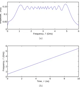
Although this description is simple, it is a vastly different approach for describing signals from traditional Fourier methods. This difference is highlighted by analyzing a linear chirp, a signal which is commonly used in radar systems:
x(t) = sin
µ
2π
µ
f0+k2t
t
. (2.5)
Fig. 2.2(b).
In this case, the Fourier description does not capture the time-varying nature of the chirp. A plateau of spectral content between 500 MHz and 5.5 GHz, with an average level ofx(t) = 0.14 and ripples of approximately 0.025 in magnitude. It is unclear from the Fourier Transform whether the signal contains components between 500 MHz and 5.5 GHz that are always present at a magnitude given by the transform, or if the signal merely spends a fraction of its time at each intermediate frequency.
The instantaneous-frequency description, on the other hand, captures the time-varying nature of the chirp. Although no amplitude information is given by (2.4), the plot follows a linear pattern as expected:
φ(t) = 2π
µ
f0+k 2t
t= 2π
µ
f0t+k 2t
2
(2.6)
ω(t) = d dt2π
µ
f0t+k2t2
= 2π(f0+kt) (2.7)
f(t) =f0+kt (2.8)
This example demonstrates that the Fourier Transform, although a powerful steady-state analysis tool, is sometimes inadequate for capturing the true nature of time-varying signals. Instantaneous frequency is one alternative way of looking at time-varying signals. Additional analysis methods are presented in Section 2.3.
2.2.2 Linear Delay: Group vs. Average
0 2 4 6 8 10 −1
−0.5 0 0.5 1
Amplitude,
x
(t)
Time, t (ns)
Figure 2.1: Linear chirp example: time-domain signal. The frequency is linearly increasing betweent= 0 andt= 10 ns.
0 1 2 3 4 5 6
0 0.05 0.1 0.15
Amplitude, |
X
(f)|
Frequency, f (GHz)
(a)
0 2 4 6 8 10
0 1 2 3 4 5 6
Frequency,
f (GHz)
Time, t (ns)
(b)
455 460 465 470 475 0
50 100 150 200 250 300 350 400 450
Group Delay (ns)
Frequency (MHz)
Figure 2.3: Group delay example: 5th-order Chebyshev filter, f
0 = 465 MHz, B = 6 MHz, passband amplitude ripple = 0.10 dB. The group delay trace peaks sharply at the edges of the filter passband. A signal with a bandwidth encompassing either/both of these points will experience linear distortion due to this sharp variation.
phase function is given byϕ(ω), its group delayτ is computed as [8]
τ(ω) =− d
dω{ϕ(ω)}. (2.9)
The group delay characteristic for a fifth-order bandpass Chebyshev filter, commonly used in Family Radio Service (FRS) radios, is given in Fig. 2.3.
If the frequency content of an input to such a circuit element is sufficiently narrow, group delay may be considered constant over the signal bandwidth. With constant group delay τ0 , the phase function of the system is approximated by
ϕ(ω)≈ −
Z
τ0 dt=−φ0−ωτ0 . (2.10)
Let the incoming signal be denoted X(ω), and the amplitude transfer function of the component be denoted |H(ω)|. The output from the component whenX(ω) is applied is
455 460 465 470 475 0
10 20 30 40 50
Voltage (mV)
Frequency (MHz)
Figure 2.4: Spectrum of a pulsed RF signal: 465 MHz tone at−10 dBm which switcheson
and off at 0.5-µs intervals. Most of the RF energy resides near the carrier frequency, but a considerable amount is spread over a wide bandwidth around the carrier.
which amounts to a scaling of the amplitude of the incoming signal by |H(ω)| , a phase shift by−φ0 , and a time delay ofτ0. This time delay is thegroup delay, the common travel time through a system for a small grouping of input frequencies. For the filter example of Fig. 2.3, a packet of frequencies near the center of the passband would take approximately 186 ns to travel from the filter input to the filter output.
If the frequency content of an input to a circuit element is not sufficiently narrow, however, group delay cannot be assumed constant over the signal bandwidth. This is the case with pulsed RF signals whose pulse frequencies approach the system’s communications bandwidth. This condition can occur in a fast-frequency-hopping scheme. An example of a pulsed signal whose travel time cannot be estimated using group delay is given in Fig. 2.4. Although most of the signal energy is concentrated within a seemingly narrow bandwidth around the fundamental tone, a significant portion of the signal energy is spread beyond this narrow band. (Here, a band of 15 MHz around 465 MHz is required to en-capsulate 98% of the signal energy.) With respect to the filter of Fig. 2.3, the group delay cannot be considered constant over the signal bandwidth. Another method for determining linear delay is needed.
error function can be formed [9]:
e(t, τ) =y(t)−x(t−τ) . (2.12)
The integral of this error squared is
ε(τ) = lim
T→∞
1 2T
Z T
−T
e2(t, τ)dt (2.13)
where τ is the delay of the signal.1 The value of τ which minimizes ε(τ) is the average delay. Unlike group delay, which is solely a property of the device and not of the applied signal, average delay depends upon both the transfer function of the device and the input waveform. Whereas the application of group delay is limited to narrowband signals, average delay can be extended to signals of arbitrary bandwidth.
Settling Time
Another time-domain quantity that is often used in the context of linear delay is
settling time,ts, which is defined as the time required for the output of a circuit to settle
within a given percentage of its steady-state amplitude upon application (or change) of a steady-state pulse at its input. Common percentages for this measure are 1/e(37%), 1/e3 (5%), and 1/e5 (1%).
Strictly speaking, settling time is not a measure of linear delay because a change of the signal at the output of a lumped-element circuit may appear (almost) instantaneously after a change in the signal at the input of the circuit, while the time required to achieve steady-state is on the order of 1/B whereB is the circuit’s bandwidth. In other words, set-tling time cannot discern between a pure-time-delay/wide-bandwidth combination (where no change in the output appears at until after the time delay, some signal appears imme-diately after the delay, and the signal settles shortly thereafter) and a narrow-bandwidth
circuit (where some signal appears immediately after the input is changed but requires approximately 1/B to achieve steady-state).
Like average delay, settling time is dependent upon both the circuit and the fre-quency of the applied signal. This property is illustrated in Chapter 3.
2.2.3 Quality Factor: Fractional Bandwidth vs. Energy Decay
Another concept that spans the time and frequency domains is quality factor, Q. Quality factor is most relevant when discussing resonant circuits. Q is a measure of the energy storage capability of a resonant structure. In a circuit, it relates the average energy stored in electric and/or magnetic fields to the energy dissipated by the system, scaled by the circuit’s resonant frequency [10]:
Q=ω(average energy stored)
(energy loss/second) . (2.14)
Qcan range from 0 — representing a circuit which stores no energy, up to∞— representing a resonant circuit which is lossless.
Q is most commonly calculated in the frequency domain as the inverse of the resonant circuit’s half-power percentage bandwidth γ,
Q= ω0 ∆ω =
1
γ (2.15)
where ∆ω is the difference between the upper and lower corner frequencies and ω0 is the center frequency of the filter. For first- and second-order circuits, the value given by (2.15) is exact, but for higher-order circuits, the value given by (2.15) is an approximation. Using this fractional-bandwidth relationship, it is straightforward to determine the quality factor of a bandpass system from scattering parameters.
to drop to 1/e of its initial value, or [11]
Q= 2π τ
T0 =ω0τ (2.16)
whereτ is the time constant of the energy decay andT0 is the period of the RF excitation at the circuit’s resonant frequency.
A misunderstanding arises when using the fractional-bandwidth relationship given by (2.15) in order to approximate the settling time of the resonant circuit by (2.16). It should be noted that the time-domain definition is strictly validfor first- and second-order resonant circuits only. For higher-order resonant structures, e.g. circuits containing three or more reactive elements, the expression in (2.15) is an approximation which worsens as the number of reactive elements in the circuit increases. The extent of the error in this approximation is evident when applying RF pulses to narrowband filters. This error is addressed in greater detail in Chapter 3.
2.2.4 Summary
In this section, a number of time-frequency quantities were defined. The term
frequency appears in every chapter of this work. Linear delay is most relevant in Chapter 3 when discussing the transit time of pulses through bandpass filters and in Chapter 4 when discussing the extraction of resonant circuit parameters from pulse-decay waveforms. The
quality factor of a coupled-resonator structure is discussed in Chapter 3, while the Q of a single resonator is emphasized in Chapter 4. Chapters 5 and 6 rely less on this terminology and more on nonlinear circuit concepts.
2.3
Review of Analysis Techniques
2.3.1 Short-Time Fourier Transform
The Short-Time Fourier Transform (STFT) is a modification of the Fourier Trans-form that is used for finite time-series data. Multiplying the original signal by a windowing function isolates a portion of the signal to be broken into Fourier components [12]:
X(τ, ω) =
Z +∞
−∞
x(t)w(t−τ)e−jωtdt (2.17)
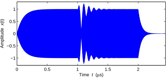
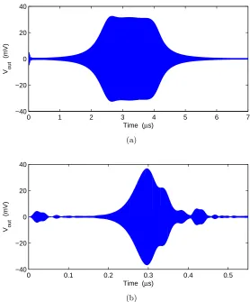
where w(t) is a windowing function centered on the time period over which the STFT is to transform the time-series data. The variable τ is used to shift the window in time. An example of the STFT is given in Figs. 2.5-2.7. The signal is written
x(t) =
£
1−e−t/100 ns¤cos¡2π·888·106t¢ 0≤t≤1µs
£
e−(t−1µs)¤cos¡2π·888·106t¢
+£1−e−(t−2µs)/50 ns¤sin¡2π·900·106t¢ 1µs≤t≤2µs
£
e−(t−2µs)/50 ns¤sin¡2π·900·106t¢ 2µs≤t≤3µs.
(2.18)
The signal x(t) consists of two sinusoids which are active at two different times. The first sinusoid at 888 MHz ramps to an amplitude of 1, following a first-order exponential rise with a time constant of 100 ns. This sinusoid ramps back down to zero after 1 µs. As the first sinusoid dissipates, the second at 900 MHz ramps up to an amplitude of 1. This sinusoid reaches its maximum value at a faster rate, a time constant of 50 ns. It ramps back down after another 1 µs.
The STFT ofx(t) without any window, which is the standard Fourier Transform, is shown in Fig. 2.6. The STFT of this signal, using a 100-ns rectangular window given by
w(t) =
(
1 τ −50 ns≤t≤τ + 50 ns
0 0.5 1 1.5 2 −1
−0.5 0 0.5 1
Amplitude
x
(t)
Time t (µs)
Figure 2.5: Short-Time Fourier Transform example: signal given by (2.18). The signal ramps up at one frequency, ramps down while ramping up at a second frequency, and ramps down at the second frequency.
880 885 890 895 900 905 910 0
0.1 0.2 0.3 0.4
Amplitude |
X
(
ω
)|
Frequency ω/2π (MHz)
Figure 2.6: Short-Time Fourier Transform of the signal in Fig. 2.5: no windowing. Both frequencies are present in this view.
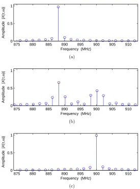
for several different values of τ, is shown in Fig. 2.7.
The Fourier Transform of Fig. 2.6 reveals that the signal contains frequency content concentrated at 888 MHz and 900 MHz. It accurately extracts the signal’s underlying sinusoids, but it does not show that each sinusoid is present for only a fraction of the data collection period. Performing the STFT on the signal using different values of the delay variable τ, however, reveals this information.
875 880 885 890 895 900 905 910 0
0.5 1
Amplitude |
X
(
τ
,
ω
)|
Frequency (MHz)
(a)
875 880 885 890 895 900 905 910 0
0.5 1
Amplitude |
X
(
τ
,
ω
)|
Frequency (MHz)
(b)
875 880 885 890 895 900 905 910 0
0.5 1
Amplitude |
X
(
τ
,
ω
)|
Frequency (MHz)
(c)
in the neighborhood of the transition time between the two sinusoids, as in Fig. 2.7(b), the STFT displays two peaks, showing that as time progresses, the presence of the first sinusoid is diminished while the presence of the second sinusoid is augmented.
Whereas the full Fourier Transform was unable to capture the time-varying nature of the signal, the Short-Time Fourier Transform (with appropriate windowing) was able to extract the frequency transitions. As evidenced by this example, the STFT is useful for analyzing signals that are sinusoidal over short durations. If the underlying frequency content is not sinusoidal, however, a more general transform is needed to extract time-frequency information.
2.3.2 Wavelet Transform
One such generalized transform which is not restricted to sinusoidal basis functions is the Wavelet Transform. It is written [13]
W(κ, τ) =
Z +∞
−∞
x(t)ψ(κ, τ, t)dt (2.20)
whereψis thewavelet(the basis function of the transform),τ is the position of the wavelet in time, and κ is thescale of the wavelet.
The Wavelet Transform can be thought of as a correlation of a recorded signal, x(t), with scalings of a pre-defined waveform,ψ(t). The higher the value ofW, the higher the degree of similarity exists betweenx(t) andψ(t) for a particular scalingκat a particular location in time τ. The wavelet must be zero-mean in order for the integral to assume a minimal value when x(t) and ψ(t) are uncorrelated.
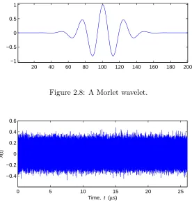
Although wavelets are similar to sinusoids in that both are zero-mean, wavelets are unlike the sinusoids of Fourier analysis because they have limited duration. The sinusoids of Fourier analysis exist for all time (or over the entire window for the STFT). An example wavelet is shown in Fig. 2.8.
20 40 60 80 100 120 140 160 180 200 −1
−0.5 0 0.5 1
Figure 2.8: A Morlet wavelet.
0 5 10 15 20 25
−0.4 −0.2 0 0.2 0.4 0.6
x
(t)
Time, t (µs)
Figure 2.9: Linear chirp from 1 to 8 GHz over 14 µs, starting at t= 6 µs, with Gaussian white noise; |x(t)|= 0.01, σn = 0.02, µn = 0. The chirp signal is not visible within the
noise.
Wavelet analysis is particularly useful for discerning patterns in a signal which follow a zero-mean shape that is not necessarily sinusoidal.
One such example is wavelet analysis of a reflected wideband linear chirp; such a signal may be found in radar applications. Assume that the received signal consists of some portion of the original transmitted chirp, the original chirp changed frequency linearly at a rate of 500 MHz/µs, the delay of the reflection in time is unknown, and the received signal is buried in white Gaussian noise. Such a signal is shown in Fig. 2.9.
0 5 10 15 20 25 0
5 10 15 20
x 10−9
W
(
τ
)
Time, t (µs)
Figure 2.10: Location of the 2-to-4 GHz linear chirp, extracted from Fig. 2.9 using chirp wavelet; τ = 8 µs. The location of the signal is determined even though the waveform is buried in noise.
ψ(τ, t) =
(
sin£2π£f0+k2(t−τ)
¤
(t−τ)¤ τ ≤t≤τ +T
0 otherwise (2.21)
f0= 2·109Hz k= 500·106 Hz T = 2µs (2.22)
When (2.20) is applied to the waveform of Fig. 2.9, the result is Fig. 2.10, which shows a peak at 8 µs, exactly where the 2-to-4 GHz chirp occurs in the noisy waveform.
Here the parameterκ is not used because only one time-scaling ofψ(τ, t) is neces-sary to identify the time index of the particular waveform. If the chirp rate were unknown, ψ(τ, t) could be scaled and W(τ) could be plotted against a number of time-scalings κ in order to extract the chirp rate.
L1 C1 L3 C3 L5 C5 R
R V 0
(a)
N2
CN5 L
N1
C RN
− V1 +
RN
V 0 LN4
N3
C
(b)
Figure 2.11: 5th-order Chebyshev filter: (a) lumped-element model, (b) lowpass equivalent circuit. Bandpass series LCs correspond to lowpass series inductors and bandpass parallel LCs correspond to lowpass shunt capacitors.
2.3.3 Lowpass Prototyping
Another tool that is useful for analyzing time-frequency properties is lowpass pro-totyping. Lowpass prototyping is particularly useful in the design and analysis of filters. It is generally discussed in the frequency domain, but its usefulness extends to the time-domain as well.
Frequency Transformation
Typically, bandpass filter design begins with the filter’s lowpass prototype, a net-work of series inductances and shunt capacitances, realizing specifications of rolloff, pass-band ripple, and 1-Ω resistive terminations. A frequency transformation is then used to center the filter’s passband at the operating frequency and to accommodate a change in resistance at the filter’s input and output ports. A fifth-order lumped-element Chebyshev filter and its lowpass equivalent are shown in Fig. 4.3(a) and 4.3(b), respectively.
bandpass filter and the first capacitor of its lowpass prototype is as follows [9]:
L1 =RC γ
N1ω0 C1 = CN1
Rω0γ ω0=
1
√
L1C1
(2.23)
where R is the resistance of the input and output terminations, and ω0 is the center fre-quency of the resonator as well as that of the overall filter.
Time Scaling
It is also noted in [9] that a simple time-scaling relationship exists between (a) the envelope of the transient response of a bandpass filter, when excited by a step-modulated waveform with carrier frequency equal to the filter’s center frequency, and (b) the transient response of the filter’s lowpass equivalent, when excited by a step change in voltage. The envelope of the voltage wave across the input resistor in the bandpass case VR is a time-scaled version of the same voltage wave in the lowpass case V1:
t=α tN α= 2
ω0γ
(2.24)
wheret is the time index of the bandpass response andtNis the time index of the lowpass equivalent response.
2.3.4 Summary
In this section, several time-frequency analysis tools — which will be used to present a number of results in this dissertation — were presented. The Short-Time Fourier Transform is used to generate all of the spectral plots presented in Chapters 4, 5, and 6. Lowpass prototyping is used in Chapter 3 to derive closed-form time-domain expressions for bandpass filter transients and in Chapter 4 to extract theQ of a single resonator from a coupled-resonator structure.
2.4
Transients in Linear Narrowband Systems
In order to understand how time-frequency effects have impacted communication systems and the extent to which they have been studied, it is necessary to review prior research on narrowband transients.
2.4.1 Discovery of Transients, Quasi-Stationary Behavior
The study of transient effects in narrowband systems can be traced back at least as far as the introduction of frequency-modulation (FM) radio. In 1937, John Carson and Thornton Fry of Bell Laboratories were the first to give a mathematical treatment of distortion in frequency modulation systems [14]. Shortly after the invention of FM, they sought to compare the performance of the new scheme against amplitude modulation (AM). They argued that FM offered a better signal-to-noise ratio, assuming FM could operate over a wider bandwidth than that of traditional AM. Carson and Fry did note the existence of a transient distortion term, but neglected it in favor of analyzing the quasi-stationary signal. Much of the analysis of frequency-varying signals since Carson and Fry’s time has focused on the quasi-stationary assumption, which states that the transient behavior of a system whose input changes frequency can be approximated by smooth transitions between steady states. Let x(t) be a signal whose frequency changes with time, ω(t), which is applied to a system with steady-state transfer function H(ω):
H(ω) = |H(ω)|ejϕ(ω) (2.26)
The quasi-stationary output from the system y(t) is then
y(t) =|H[ω(t)]|A(t) cos [ω(t)·t+φ0+ϕ[ω(t)]]. (2.27)
The transient response is scaled in amplitude byH(ω) and phase-shifted by ϕ(ω) at each point in time, depending upon the input’s instantaneous frequencyω(t).
A system operates in the quasi-stationary regime as long as the input signal’s frequency varies slowly with respect to the system’s response time. Fig. 2.12 shows when this is the case and when it is not. Here a linear chirp is applied to a bandpass filter. In Fig. 2.12(a), the chirp rate is much slower than the filter’s transient response. As the input frequency changes, the magnitude of the output waveform changes with the steady-state filter response; the chirp traces out the filter’s frequency-domain transmission characteristic. In Fig. 2.12(b), however, the chirp rate approaches the transient response time of the filter. The output no longer traces out the transmission characteristic because the filter has not been given enough time to assume steady state as the input changes frequency. Because the output response is no longer a smooth transition between steady states, the quasi-stationary assumption is no longer valid.
Concurrent with Carson and Fry’s analysis, Hans Roder, a radio engineer at Gen-eral Electric, was concerned with the effect of tuned circuits on the reproduction of FM signals [15]. Instead of making the quasi-stationary assumption and using steady-state analysis, he used Bessel functions to represent oscillatory signal components propagating through frequency-to-amplitude converters and tuned amplifiers. Roder determined that, in order to reproduce an audio signal without introducing distortion, a frequency-to-amplitude converter must have linear amplitude and phase characteristics, and an amplifier must have a flat amplitude characteristic and linear phase characteristic over its full operational band-width. Unbeknownst to Roder, his analysis implied that a filter would require a constant group delay across its passband for distortionless transmission.
0 1 2 3 4 5 6 7 −40
−20 0 20 40
Vo
u
t
(mV)
Time (µs)
(a)
0 0.1 0.2 0.3 0.4 0.5 −40
−20 0 20 40
Vo
u
t
(mV)
Time (µs)
(b)
transmission and reflection properties for a filter’s passband and stopband, Salinger found that the instantaneous frequency response of a bandpass filter slowed with a decrease in filter bandwidth. He noted that the settling times of both AM and FM transients were similar as long as any input frequency swings were well within the filter’s nominal passband. Salinger recommended that a filter’s passband be chosen to enclosed the maximum input swing symmetrically. He also performed back-of-the-envelope calculations to determine the minimum operational bandwidth for FM radio, AM video with FM synchronization, and FM video.
Donald Hess, an associate professor at the Polytechnic Institute of Brooklyn, fol-lowed up on Carson and Fry’s quasi-stationary analysis [17]. Hess wanted to know the bandwidth required of single-tuned Butterworth and Chebyshev filters to transmit FM sig-nals with a specified amount of phase distortion. He derived a tighter error bound than Stumpers, and calculated that the experimental requirement of 225 kHz bandwidth for clean FM transmission matched the theoretical requirement for less than 1% phase distortion.
2.4.2 Circuit Solutions
Circuit solutions addressing transient distortion began to appear in the late 1940s. Gordon Tucker, a communications researcher for the British Post Office Research in Lon-don, presented a mathematical treatment of a commonly-used 6-element (i.e. non-ideal) filter excited by single-tone pulses [18, 19]. Tucker used differential operators (a precursor to Laplace Transforms) to find analytical expressions for the build-up and decay charac-teristics of the filter’s transmissions at midband. He also provided the first oscilloscope traces of a bandpass filter’s pulse transmissions. Charles Eaglesfield of the Mullard Radio Valve Company in London picked up on Tucker’s work and gave an analytical form for the amplitude of the transmitted pulses, assuming a narrowband case [20, 21].
bounds for Carson and Fry’s quasi-static solution [23].
Several years later, in 1951, William Hatton at the Massachusetts Institute of Technology was considering FM as a way to transmit video and wanted to compare its performance against AM [24]. Hatton analyzed the response of a parallel RLC circuit to a single discrete frequency step by solving the circuit’s differential equation directly. Using settling time and overshoot of the output’s instantaneous frequency as metrics, he found that FM and AM perform similarly when jumps in the input frequency are small and near the center of a filter’s passband, but FM outperforms AM for larger input frequency swings. He saw that overshoot in the amplitude response could be as high as 10% above steady-state values, even if the operating frequencies are kept within the passband.
2.4.3 Laplace Methods
Laplace Transforms were applied to circuit transients in the 1950s. While engaged in radar-system research at the Hughes Aircraft Company in 1954, R. E. McCoy analyzed FM distortion in stagger-tuned amplifiers [25]. He noticed that, when exciting a tuned circuit by a discrete frequency step, that the shape of the output frequency transient was dependent upon (a) the initial frequency of the step, (b) the magnitude of the step, and (c) the direction of the step. He derived a circuit solution for normalized output frequency deviation using the inverse Laplace Transform, which could be generalized to tuned circuits with any number of stages. McCoy provided detailed computations for large frequency steps in single-tuned circuits. He showed how the frequency transient is longer when using more stages and recommended that stagger-tuning not be used if distortion is to be kept to a minimum.
single-tuned circuit and a series of frequency steps.
Harry Hartley of the Westinghouse Electric Corporation in Baltimore presented another simplification of the Laplace Transform method in 1966 [27]. He exploited several properties of Laplace Transforms under narrowband assumptions for both the input signal and the system’s transfer function to determine the instantaneous amplitude, phase, and frequency of output transients.
The Laplace Transform of a system’s output Vo(s) is, in general, the product of a transfer function H(s) with an input excitation Vi(s):
Vo(s) =Vi(s)H(s). (2.28)
Vo(s) may be written as the ratio of two polynomials whose roots are the poles and zeros
of Vo(s). It is noted in [27] that, for linear narrowband circuits, all zeroes and poles of the system are (a) clustered in a narrow frequency band, (b) are real or complex conjugates of each other, and (c) have either a zero or negative real part. This allows the system’s output to be written
Vo(s) =K
Q
m
(jω0+σ0m)Q
n
(jω0−s∗
0n) (s−s0n)
Q
i
(jω0+σpi)Q
j
³
jω0−s∗ pj
´
(s−spj) (2.29)
vo(t) =<
"
1 πj
Z c+j(ω0+B/2)
c−j(ω0−B/2)
Vo(s)etsds
#
(2.30)
where σ0m are the real zeros of Vo(s), s0n are the complex conjugate zeros, σpi are the
characteristics could impact frequency-shift-keying communication schemes.
Chohan and Fidler at the University of Essex in England went further in assessing the suitability of bandpass filters for use in frequency- and phase-modulated communications [28]. They focused on the instantaneous frequency of the output and used the s-domain shifting property of Laplace Transforms to generalize Hartley’s instantaneous frequency result to filters of any order and any Q value. They provided simulated data for second-order Butterworth filters.
2.4.4 Summary & Current Research
Transients in narrowband circuits have been observed as early as the 1930s. Dif-ferential equations and Laplace methods have been used to determine the extent to which these transients will distort communication systems, but most work has been limited to lower-order systems for mathematical tractability.
Studies of transient distortion have not yet been extended to higher-order band-pass filters, and no data have yet been presented to evaluate the effects of such distor-tion on frequency-hopped communicadistor-tions for filters of any design. Because higher-order narrowband filters have become so common to wireless device architectures, and because frequency-hopping systems that implement such filters may fail if circuit transients are longer than anticipated, an evaluation of narrowband linear effects produced by contem-porary filter designs is performed in Chapter 3 and an evaluation of narrowband nonlinear effects is performed in Chapter 5.