Real-Time Embedded Systems
Design Principles and Engineering Practices
Xiaocong Fan
AMSTERDAM • BOSTON • HEIDELBERG • LONDON NEW YORK • OXFORD • PARIS • SAN DIEGO SAN FRANCISCO • SINGAPORE • SYDNEY • TOKYO
225 Wyman Street, Waltham, MA 02451, USA Copyright©2015 Elsevier Inc. All rights reserved.
No part of this publication may be reproduced or transmitted in any form or by any means, electronic or mechanical, including photocopying, recording, or any information storage and retrieval system, without permission in writing from the publisher. Details on how to seek permission, further
information about the Publisher’s permissions policies and our arrangements with organizations such as the Copyright Clearance Center and the Copyright Licensing Agency, can be found at our
website:www.elsevier.com/permissions.
This book and the individual contributions contained in it are protected under copyright by the Publisher (other than as may be noted herein).
Notices
Knowledge and best practice in this field are constantly changing. As new research and experience broaden our understanding, changes in research methods, professional practices, or medical treatment may become necessary.
Practitioners and researchers must always rely on their own experience and knowledge in evaluating and using any information, methods, compounds, or experiments described herein. In using such information or methods they should be mindful of their own safety and the safety of others, including parties for whom they have a professional responsibility.
To the fullest extent of the law, neither the Publisher nor the authors, contributors, or editors, assume any liability for any injury and/or damage to persons or property as a matter of products liability, negligence or otherwise, or from any use or operation of any methods, products, instructions, or ideas contained in the material herein.
British Library Cataloguing in Publication Data
A catalogue record for this book is available from the British Library Library of Congress Cataloging-in-Publication Data
A catalog record for this book is available from the Library of Congress ISBN: 978-0-12-801507-0
For information on all Newnes publications visit our website at http://store.elsevier.com/
Typeset by SPi Global, India Printed and bound in USA
Preface
An embedded system is an electronic system that is designed to perform a dedicated function within a larger system. Real-time systems are those that can provide guaranteed worst-case response times to critical events, as well as acceptable average-case response times to noncritical events. When a real-time system is designed as an embedded component, it is called a real-time embedded system. Real-time embedded systems are widespread in consumer, industrial, medical, and military applications.
As more and more of our daily life depends on embedded technologies, the demand for engineers with the skill set for the development of real-time embedded software has soared in recent years. As a consequence, preparing students for the design and implementation of embedded software is becoming increasingly important. This textbook is written especially for advanced undergraduates or master-level students who are pursuing a major in software engineering, computer engineering, or a related discipline. The textbook may also benefit practicing engineers with a concentration in embedded software development.
This book takes a synergetic approach to introducing ideas and topics from real-time systems, embedded systems, and software development principles. Readers will not only gain a thorough understanding of concepts related to microprocessors, interrupts, and the
cross-platform development process, and appreciate the importance of real-time modeling and scheduling, they will also be trained in good software engineering practices such as model documentation, model analysis, design patterns, and system standard conformance.
This textbook features three aspects that are essential for the development of real-time embedded software.
First, developing software for real-time embedded systems involves many activities, including specification of requirements, timing analysis, architecture design, multitasking design, and cross-platform testing and debugging. This book covers the whole process of embedded software development, with some topics fully explained and others only briefly mentioned (e.g., debugging and testing). In particular, this book presents various embedded software architectures in a systematic way, with a focus on a real-time operating system, which is the most advanced architecture adopted in large real-time embedded systems. Moreover, we have chosen to place significant emphasis on reusable design solutions. As shown in Table0.1, this
Table 0.1 Summary of design patterns
Category Pattern Name Where in the Book
ISR
ISR-Pattern-min Section 4.5.1
ISR-Pattern-server Section 4.5.2
Interrupt chaining Figure 4.7 in Section 4.5.3 Interrupt cascading Figure 4.9 in Section 4.5.4 Interrupt disabling Figure 4.11 in Section 4.5.5
Double buffering Figure 4.12 in Section 4.5.5 Honor first request Figure 12.17 in Section 12.3.2
Subclassing Abstraction-occurrence Figure 6.25 in Section 6.3.4
General hierarchy Figure 6.27 in Section 6.3.4
Software architecture
Round-robin DAS Figure 12.10 in Section 12.2.2 Round robin with interrupts Figure 12.16 in Section 12.3.2 FIFO queuing Figure 12.20 in Section 12.4.1 Priority queuing Figure 12.21 in Section 12.4.2 Serial port design pattern Figure 14.5 in Section 14.2.2.1
Static task scheduler
Clock based Section 15.2
Frame based Section 15.3
Timing wheel Section 22.3
Semaphore/mutex Rendezvous synchronization pattern Figure 18.8 in Section 18.3.1 Multi-instance resource protection Figure 18.19 in Section 18.4.1
Condition variable
Barrier synchronization pattern Figure 18.24 in Section 18.5.1 Producer-consumer pattern Figure 18.25 in Section 18.5.2 Read-write lock pattern Figure 18.30 in Section 18.5.3
Message queue
Unidirectional queuing pattern Figure 19.5 in Section 19.3.1 Acked-unidirectional queuing pattern Figure 19.6 in Section 19.3.2 Bidirectional queuing pattern Figure 19.7 in Section 19.3.3 Client-server queuing pattern Figure 19.10 in Section 19.3.4
Pipe Unidirectional piping pattern Figure 20.3 in Section 20.3 Bidirectional piping pattern Figure 20.3 in Section 20.3 Deadlock avoidance Hierarchical messaging pattern Figure 21.8 in Section 21.7.3
DAS, detect-acknowledge-service; FIFO, first in first out; ISR, interrupt service routine.
book introduces many design patterns, which represent the best practices that can be reused in a wide range of real-time embedded systems.
Third, POSIX (for “portable operating system interface”) is an open operating system interface standard that has been developed to promote interoperability and portability of applications across variants of Unix operating systems. Software systems built upon one real-time operating system can be easily ported to other POSIX-compliant operating systems. This text features POSIX.1-2008 (2013 edition). The operating system services and concepts covered in this book are fully compatible with the POSIX.1-2008 standard. The example codes provided in this book have been tested in QNX—a real-time operating system widely adopted in industry. Since QNX is POSIX compliant, the programs may also be compiled, without changing the source code, for execution on another POSIX-compliant operating system.
Briefly, this textbook consists of four parts:
• Part I is dedicated to a basic introduction to real-time embedded systems and the iterative development process. Although our emphasis is on the software aspects, complete
isolation from the underlying hardware is neither feasible nor desirable. For such a reason, this part also contains two chapters on microprocessors and interrupts—fundamental topics for software engineers who wish to build embedded systems.
• Part II is dedicated to modeling techniques for real-time systems. In particular, we introduce the modeling tools covered by UML—a standard widely adopted in both academia and the software industry. Moreover, we introduce real-time UML—a profile for specifying real-time-related constraints in system models. UML diagrams are consistently used throughout the book to illustrate key concepts and design patterns. • Part III is dedicated to the design of software architectures for real-time embedded
systems. We start with generic architectures, which lead us to the most complicated architecture—a real-time operating system. The focus is then switched to multitasking and real-time scheduling—two critical issues to be addressed by any designers of real-time embedded systems.
• Part IV is dedicated to system implementation. We especially focus on those mechanisms available on any POSIX-compliant operating systems; this means that the
design/implementation patterns given in this book are applicable to other POSIX-compliant operating systems as well.
To aid instructors and students in using this text, we provide a supplements package on Elsevier’s companion website: http://booksite.elsevier.com/9780128015070. This package includes PowerPoint slides and source code.
In this text, I have not been able to cover every major topic concerned with real-time
embedded systems. I have exercised my best judgement in deciding which topics are suitable for software engineers, which to emphasize, and which to omit. Seriously interested readers may refer to other textbooks for different perspectives.
Comments from colleagues are encouraged and welcome. Please feel free to send suggestions to Xiaocong Fan, Behrend College, Pennsylvania State University, Erie, PA 16563, USA (e-mail: [email protected]). I look forward to hearing from you about your experiences with the text.
Acknowledgments
First of all, I am grateful for the opportunity to learn from many excellent texts available on real-time systems or embedded systems, the authors including Jane W.S. Liu, David E. Simon, Rob Williams, Qing Li, and Bruce P. Douglass, to mention only a few. They may recognize their influence in some parts of the book, directly or indirectly.
I am indebted to the reviewers for numerous comments and enlightening suggestions. I would like to thank my students, who have been influential in shaping my thoughts on how best to organize and teach a course on real-time embedded systems.
The final manuscript was ably edited by SPi. A most special thanks go to Tim Pitts, Charlie Kent and Nicky Carter at Elsevier. This book would not be possible without their graceful management and great patience.
Acronyms
AIC Advanced interrupt controller
ANSI American National Standards Institute
BSP Board support package
CAN Controller area network
CISC Complex instruction set computing
COFF Common Object File Format
COM Serial communication port
CPU Central processing unit
CSPR Current program status register
DAS Detect-acknowledge-service
DMA Direct memory access
DSP Digital signal processor
DTCM Data tightly coupled memory
EDF Earliest deadline first
EEPROM Electrically erasable programmable read-only memory
ELF Executable and Linking Format
EOI End of interrupt
EPROM Erasable programmable read-only memory FIFO First in first out
GPR General-purpose register
GRM General Resource Modeling
GRM Graphical user interface
HLP Highest locker protocol
HNERT Highest-priority nonempty ready-thread list I2C Inter-Integrated Circuit
IC Integrated circuit
ICE In-circuit emulator
ICR Interrupt command/status register
IEEE Institute of Electrical and Electronics Engineers
IMR Interrupt mask register
INV Interrupt vector number
IP Internet Protocol
IQR Interrupt request
IRR Interrupt request register ISR Interrupt service routine
LNA Low-noise amplifier
LSb Least significant bit LSB Least significant byte
MMU Memory management unit
MOF Meta Object Facility
MSB Most significant byte
NVM Nonvolatile memory
OCL Object Constraint Language
OMG Object Management Group
OOM Object-oriented modeling
OOP Object-oriented programming
OS Operating system
PC Personal computer
PCP Priority ceiling protocol PCR Program counter register PDF Probability distribution function PIC Programmable interrupt controller PIT Programmable interval timer POSIX Portable Operating System Interface PRF Pulse repetition frequency
QoS Quality of service
RAM Random-access memory
RF Radio frequency
RISC Reduced instruction set computing
RMA Rate-monotonic assignment
ROM Read-only memory
RTOS Real-time operating system
RT-UML Real-time Unified Modeling Language SFR Special-function register
SPI Serial peripheral interface SRAM Static read-access memory
TCM Tightly coupled memory
UART Universal asynchronous receiver-transmitter
UML Unified Modeling Language
Introduction to Embedded and Real-Time
Systems
Contents
1.1 Embedded Systems 3
1.2 Real-Time Systems 5 1.2.1 Soft Real-Time Systems 5 1.2.2 Hard Real-Time Systems 6 1.2.3 Spectrum of Real-Time Systems 7
1.3 Case Study: Radar System 8
Part of the joy of looking at art is getting in sync in some ways with the decision-making process that the artist used and the record that’s embedded in the work.
Chuck Close
1.1 Embedded Systems
In computing disciplines (computer engineering, software engineering, computer science, information systems and technology), the term “embedded system” is used to refer to an electronic system that is designed to perform a dedicated function and is often embedded within a larger system.
Embedded systems differ from general-purpose computing devices mainly in two aspects:
• First, an embedded system is designed simply for a specific function, whereas a
general-purpose computing device, such as smartphone, laptop, or desktop computer, is not; they can be used as Web servers or data warehouses, or can be used for writing articles, reading news, playing games, or running scientific experiments, to mention only a few applications.
• Second, an embedded system is traditionally built together with the software intended to run on it. Such a parallel model of developing hardware and software together is known as hardware-software co-design. Recently, there has been a trend where an embedded system
Real-Time Embedded Systems. http://dx.doi.org/10.1016/B978-0-12-801507-0.00001-8 ©2015 Elsevier Inc. All rights reserved.
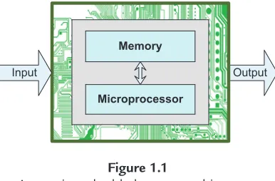
Figure 1.1
A generic embedded system architecture.
is built with awell-defined interfaceopen to third-party embedded software providers. In contrast, a general-purpose computing device is often built independently from the software applications that may run on it.
An embedded system is a combination of computer hardware and software, and sometimes mechanical components as well.Figure 1.1gives a bird’s-eye view of a generic embedded system architecture, where the microprocessor and the memory blocks are the heart and the brain, respectively. Embedded software is commonly stored in nonvolatile memory devices such as read-only memory (ROM), erasable programmable ROM (EPROM), and flash memory. The microprocessor also needs another type of memory—random-access memory (RAM)—for its run-time computation.
When an embedded system is powered on, its microprocessor reads software instructions stored in memory, executes the instructions to process input information from peripheral components (through sensors, signals, buttons, etc.), and produces output to meet the needs of the externalembeddingsystem.
Given that the hardware components are chosen, most of the design effort is in the software, including application, device drivers, and sometimes an operating system. In many cases, it is possible to build a customized integrated circuit (IC) that is functionally equivalent to an embedded system. An IC-based solution is a hardwired solution that does not contain software and a microprocessor. However, the embedded system solution is more flexible and less expensive, especially when the product needs to be frequently upgraded to accommodate new changes. In response to a new change, for the hardwired solution, a new circuit needs to be designed, constructed, and delivered. In contrast, for the embedded system solution, software patches can be rapidly developed, and the upgrading process can be done over the Internet and may typically take just a few seconds.
opener, TV remote control, microwave oven, programmable thermostat, Xbox controller, and USB memory card reader. This list goes on and on.
Someone said that there are more computers in our homes and offices than there are people who live and work there. If this is true, then there are even more embedded systems that have been and will continue changing every part of our lives. One proof of this statement is that about 98% of microprocessors go into embedded systems, whereas less than 2% of microprocessors are used in computers.
1.2 Real-Time Systems
There are systems that need to respond to a service request within a certain amount of time: they are called real-time systems [22, 45]. To a real-time system, each incoming service request imposes a task (job) that is typically associated with a real-time computing constraint, or simply called its timing constraint.
The timing constraint of a task is normally specified in terms of its deadline, which is the time instant by which its execution (or service) is required to be completed. Depending on how serious missing a task deadline is, a timing constraint can be either a hard or a soft constraint:
• A timing constraint ishardif the consequence of a missed deadline is fatal. A late response (completion of the requested task) is useless, and sometimes totally unacceptable.
• A timing constraint issoftif the consequence of a missed deadline is undesirable but tolerable. A late response is still useful as long as it is within some acceptable range (say, it occurs occasionally with some acceptably low probability).
Actual systems may have both hard and soft timing constraints. A system in which all tasks have soft timing constraints is a soft real-time system. A system is a hard real-time system if its key tasks have hard timing constraints.
1.2.1 Soft Real-Time Systems
A soft real-time system offersbest-effortservices; its service of a request isalmost always
completed within a known finite time. It may occasionally miss a deadline, which is usually considered tolerable. It is worth noting that although missing a deadline will not cause catastrophic effects, the usefulness of a result may degrade after its deadline, thereby degrading the system’s quality of service.
Table 1.1 Example soft real-time systems
Example System Example Timing Constraint Consequence of Missed Deadlines
Digital camera
Shutter speed, shown in seconds or fractions of a second, is a measurement of the time the shutter is open. When the shutter speed is set to 0.5 s, the shutter open time should be (0.5±0.125) s 99.9% of the time
Unsatisfied users may switch to other models
Global positioning system
Upon identifying a waypoint, it can remind the
driver at a latency of 1.5 s The driver misses the waypoint Robot-soccer
player
Once it has caught the ball, the robot needs to kick the ball within 2 s, with the probability of breaking this deadline being less than 10%
Its team may lose the game
Wireless router The average number of late/lost frames is lessthan 2/min
The user has bad Web surfing experience
1.2.2 Hard Real-Time Systems
In a hard real-time system, missing some deadlines is completely unacceptable, because this could result in catastrophic effects such as safety hazards or serious financial consequences.
A hard real-time system offersguaranteedservices. Hence, the correctness of a hard real-time system is twofold: functional correctness and timing correctness. Here, the timing correctness of a system means that its service of a request is guaranteed to be completed within a strict deadline. Actually, in most cases timing correctness is even more important than functional correctness, because a partially functional system may be used as is and still has its values, whereas a fully functional system is useless if the offered services have no guaranteed service completion time.
Since breaking a hard timing constraint is unaffordable, it is normally a requirement that the designers/developers of a hard real-time system shouldvalidate rigorouslythat the system can meet its hard timing constraints. In the literature, the proof techniques include design-time schedulability analysis, exhaustive simulation, combinatorial performance testing, and symbolic reasoning tools based on temporal logics (e.g., model checking). While many of these techniques are beyond the scope of this book, we will cover basic approaches to schedulability analysis when it comes to real-time scheduling.
Hard timing constraints are typically expressed in deterministic terms.Table 1.2gives some example hard real-time systems.
Table 1.2 Example hard real-time systems
Example System Example Timing Constraint Consequence of Missed Deadlines
Antilock braking system
The antilock braking system should apply/ release braking pressure 15 times per second A wheel that locks up should stop spinning in less than 1 s
Loss of human lives
Antimissile system
It never needs more that 30 s to intercept a missile after it reenters the atmosphere (in the terminal phase of its trajectory)
Loss of human lives, huge finan-cial loss
Cardiac pacemaker
The pacemaker waits for a ventricular beat after the detection of an atrial beat. The lower bound of the waiting time is 0.1 s, and the upper bound of the waiting time is 0.2 s
Loss of human life
FTSE 100 Index It is calculated in real time and publishedevery 15 s Financial catastrophe
compute only an approximate firing range, which demands more weapons being activated to cover the firing range. Since the first approach consumes fewer resources, it is the default approach employed by the system to handle incoming missiles. However, the system would switch to the second approach if it predicts that waiting for the precise calculation would take too much time for the incoming missiles to be safely destroyed.
In contrast, for a soft real-time system, it typically does not take any corrective actions until the bad thing really happens. For example, a DVD player has to synchronize the video stream and the audio stream. A missed deadline happens when, owing to data loss or decoding latency, the timing difference of the two streams exceeds a certain tolerable threshold. After a missed deadline has been detected, a DVD player may selectively discard the decoding of some video/audio frames to resynchronize the two streams.
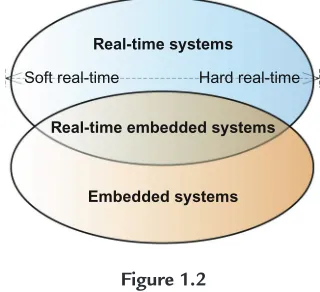
1.2.3 Spectrum of Real-Time Systems
A real-time system is called areal-time embedded systemif it is designed to be embedded within some larger system.
Real-time systems
Real-time embedded systems
Embedded systems
Soft real-time Hard real-time
Figure 1.2
System classification.
1.3 Case Study: Radar System
Radar (radiodetectionandranging) is an object-detection system that uses radio waves or microwaves to determine the distance range, altitude, direction, or speed of objects. Radar has been widely used in many areas, including airport traffic control systems, aviation control systems, military surveillance systems, antimissile systems, and meteorological precipitation monitoring.
Radar is a very complex electronic and electromagnetic system [51, 58, 70]. Below we briefly describe the functionality of each subsystem. Readers may choose to skip the details for now, but will find them useful when we use radar as an example to explain advanced modeling concepts later in the book.
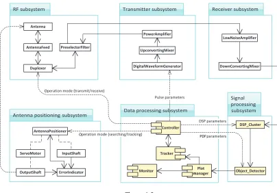
As shown inFigure 1.3, a radar system is typically composed of several subsystems.
Theradio frequency (RF) subsystemgenerally consists of an antenna, an antenna feed, a duplexer, and some preselector filters. The antenna is the interface with the medium of radio wave propagation, and it is the first stage during signal reception and the last stage during signal transmission. The antenna feed collects energy as it is received from the antenna, or transmits energy as it is transmitted to the antenna. The duplexer switches the radar system between transmit mode and receive mode. The switch operation must be extremely
rapid—say, within 5 ms (a real-time constraint)—in order to detect or track fast-moving targets. The switch operation frequency can be adjusted by an operator through the controller, which is part of the data processing subsystem. Preselector filters are used to attenuate out-of-band signals and images during the signal reception phase, and during transmission they are used to attenuate harmonics and images.
p p p
O
O PDF
m
Figure 1.3
A radar system: its components, information flow (solid lines), and control flow (dashed lines).
N
Figure 1.4
The radar signal in the time domain.
frequency). The generated signals must conform to the timing constraints specified in the design. The upconverting mixer is used to transform the baseband frequency signals into RF signals. The power amplifier is used to amplify the RF signals for transmission.
constrains the radar’s maximum detection range. The pulse width also determines the dead zone at close range. A radar echo takes approximately 1µs to return from a target 150 m away. This means if the radar pulse width is 1µs, the radar will not be able to detect targets closer than 150 m because the receiver is blanked while the transmitter is active.
The pulse repetition frequency (PRF) is the rate of pulse transmission. Most radar systems emit pulses multiple times in each direction so that multiple echo signals can be received. While a radar system might not be able to detect a target on the basis of simply one echo signal, the integration of multiple reflected pulses (of similar amplitudes) can reinforce the return signals and make detection easier. PRF can range from a few kilohertz to tens or hundreds of kilohertz. For example, a radar with a 1◦horizontal beamwidth that sweeps the entire 360◦horizon every second with a PRF of 2160 Hz can emit six pulses over each 1◦arc; it thus can receive six echoes from each target within the detection range. Note that the (unambiguous) detection range is reduced as the PRF is increased because the receiver active period is shortened. A lower PRF gives a longer detection range, but often suffers from poorer target painting and velocity ambiguity.
Modern radar systems often use a technique calledPRF staggering. With staggered PRF, the transmitter can use different PRFs to produce packets: a packet of pulses is transmitted with a fixed interval between pulses, and then another packet is transmitted with a slightly different interval. By PRF staggering, a radar can force the “jamming” signals from other radar systems to jump around erratically, inhibiting integration and thus suppressing their impacts on target detection. The PRF parameters can be set up by human operators and automatically adjusted by the controller of the data processing subsystem.
Thereceiver subsystemconsists of a low-noise amplifier (LNA) and a downconverting mixer. After signal transmission, a radar system typically positions its antenna in that direction for a few milliseconds up to a few hundreds of milliseconds to collect the echo signals (such a dwell time is another example of a real-time constraint). Echo signals often contain noises. The LNA is used to separate desired signals from undesired signals, such as thermal noise, clutter (echoes returned from objects that are not targets of interest, such as precipitation and birds), and interference (signals originating from active sources other than the radar). The LNA can also boost the power of the desired signals without introducing undesired distortions. The downconverting mixer is used to transform the RF signals into baseband frequency signals. Finally, the receiver subsystem uses A/D converters to sample an analog signal and save the digital values in shared memory accessible to the signal processing subsystem.
torque on the output shaft in a direction to reduce the error. Through the controller, an operator can change the operation mode of the antenna positioner (say, from searching to tracking a target), or can alter the scan strategy (say, a conical scan, a unidirectional sector scan, or a circular scan).
Echoes from targets must be detected and processed before the transmitter emits the next pulse. After transmission of a pulse, if there is a reflective object (say, an unmanned aerial vehicle) at a distance ofxmeters from the antenna, the echo signal reflected by the object returns to the antenna in approximately 2x/cs, wherec=3×10⁸ m/s is the speed of light in a vacuum. To measure the target distance, the radar’s detection range is divided into many
range intervalsor range bins, the length of which is equal to the desired range resolution (say, 200 m). The antenna’s pulse repetition period can then be divided into many time frames, where the length of a time frame equals the time it takes the radio signal to propagate exactly one range interval. The digital values collected within each time frame form one sample of the situation in the corresponding range bin. Since the radar can transmit pulses multiple times in each direction, multiple samples for each range bin can be collected, and these are the inputs to thesignal processing subsystem.
In general, the number of range bins can be in the hundreds or even thousands, and PRFs can range from a few to tens or hundreds of kilohertz. Such a high-demanding real-time constraint typically requires many digital signal processors (DSP) to form a computing cluster. The DSP cluster needs to produce a discrete Fourier transform of the samples for each range bin, and calculate the frequency spectrum of the echoes.
Theobject detectorcan determine whether there are objects in the direction in which the antenna is pointing and their positions and velocities, if applicable. If there is a moving object, the frequency of the reflected signal must be different from the frequency of the transmitted signal, which is called Doppler shift. The amount of Doppler shift is proportional to the velocity of the object.
A statistical hypothesis testing approach can be used to determine whether or not a
measurement represents the influence of a target or merely interference [58]. The decision rule is simple: if the calculated “likelihood ratio” exceeds the detection threshold, declare a target to be present; otherwise, declare that a target is not present. Notice that the object detector relies on several unknown parameters that need to be replaced by their maximum likelihood estimates. The probability distribution functions that form the likelihood ratio may depend on one or more parameters. The position of the threshold can be dynamically adjusted to
Thedata processing subsystemis used to track targets of interest, interact with human operators, generate commands to control the radar, and adjust parameters of the other subsystems.
The controller module is the kernel of the radar system; it is not only responsible for
synchronizing the behavior of the whole system to meet various timing constraints, but is also critical in tuning the performance of each component by adjusting certain parameters. For instance, it can alter the signal processing parameters such as the detection threshold and transform types, as well as the parameters for the statistical models used by the object detector. In addition, it can regulate the behavior of the digital waveform generator by changing the pulse parameters (such as the pulse width, pulse frequency, PRF, etc.).
The role of the plot manager is to manage real-time updates (also called plots) received from the object detector (say, once every 5 s) of the signal processing subsystem. The monitor module can be connected to a decision-support system so that human operators can make sense of the current situation and make real-time decisions.
The role of the tracker module is to process plots and to determine which plot belongs to which target, while rejecting any false alarms. Tracking is a computationally intensive activity, which typically has several steps:
• Track prediction.The tracker keeps a record (called a track) for each active target of interest. Each track has a unique ID, a state (including position, acceleration, speed, and heading), and possibly a target motion model (which is constructed to fit the motion history of the target). In this step, for each track the tracker needs to employ the associated motion model to predict its new state. It is particularly difficult when the target movement is very unpredictable or when the density of targets is high or the number of false returns is large. In such a situation, the tracker can employ a multiple-hypothesis approach where a track can be branched into many possible directions, with the most unlikely potential branches removed over time to reduce computational cost.
• Track gating.The gating process tentatively assigns a plot to an established track if the plot is within a threshold distance away from the predicted position of the track. • Track association.In practice, it is very likely that a plot is assigned to more than one
• Track initiation.After track association, a number of plots may remain unassociated with existing tracks. The tracker will create a new track for each of the unassociated plots. A new track is typically given the status of “tentative” until plots from subsequent radar updates have been successfully associated with the new track. Before being reinforced and confirmed by subsequent radar updates, tentative tracks are transparent to the operator so that false alarms can be washed away from the screen display.
• Track maintenance.Some existing tracks may be missing updates for a while (say, for the past five consecutive radar update opportunities). There is a chance that the target may no longer be there. Depending on the nature of the applications, such a track can be
terminated—say, if the target was not seen for the past five out of the 10 most recent update opportunities.
Being a real-time system, a radar system typically operates with many timing constraints at different levels. For example, the object detector may produce batches of radar updates every 5 s, and it is thus necessary for the tracker to process all those radar updates within 5 s. The cluster of DSPs may need to complete its processing at the millisecond level per round, while the receiver may need to get its job done at the microsecond level per echo signal.
Problems
1.1 What is an embedded system? Identify some embedded systems used in your everyday life.
1.2 Are the laboratory computers embedded systems? Why or why not? 1.3 Is Google Glass an example of embedded systems? Why or why not? 1.4 What is a real-time system?
(a) Identify some hard real-time systems, and for each, identify a few hard timing constraints.
(b) Identify some soft real-time systems, and for each, identify a few soft timing constraints.
1.5 What would a hard real-time system do if it anticipates that a deadline might be missed? 1.6 Explain how a radar system could be either a hard real-time system or a soft real-time
Cross-Platform Development
Contents
2.1 Cross-Platform Development Process 16 2.2 Hardware Architecture 17
2.3 Software Development 18 2.3.1 Software Design 18
2.3.2 System Programming Language C/C++ 18 2.3.2.1 Declarations and definitions 20
2.3.2.2 Scope regions 21
2.3.2.3 Storage duration 22
2.3.2.4 Linkage 22
2.3.2.5 Storage-class specifiers 23
2.3.3 Test Hardware-Independent Modules 25 2.4 Build Target Images 25
2.4.1 Cross-Development Toolchain 25 2.4.1.1 Cross compiler/assembler 25
2.4.1.2 Linker 27
2.4.1.3 Dynamic linker 28
2.4.2 Executable and Linking Format 28 2.4.2.1 Linking view 30
2.4.2.2 Execution view 32 2.4.3 Memory Mapping 34
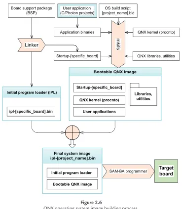
2.4.4 Case Study: Building a QNX Image 36 2.5 Transfer Executable File Object to Target 38 2.6 Integrated Testing on Target 39
2.7 System Production 39
Great computer hardware is only a doorstop without great software.
Charles King
Real-Time Embedded Systems. http://dx.doi.org/10.1016/B978-0-12-801507-0.00002-X ©2015 Elsevier Inc. All rights reserved.
2.1 Cross-Platform Development Process
Compared with nonembedded software, the development of embedded software renders many unique challenges to software engineers:
• For embedded systems, especially for real-time embedded systems, timing correctness is equally important as functional correctness. Sometimes, a timing constraint is so
important that it becomes an integral part of the functional requirements. For example, although a GPS navigation system can always identify waypoints correctly (functional correctness), it is useless if it is not able to report the waypoints before it is too late for the user to take actions.
• Most embedded systems are “dumb” devices that cannot run a debugger; this makes it hard to detect and clear program defects. For example, the processing system embedded inside a refrigerator can handle inputs from its touchpad and door sensor, provide output to a digital display, and control the cooling and icemaker machinery. It, however, may not have “luxurious” resources reserved for debugging.
• Most embedded systems are required to offer high reliability. For example, if a system has a reliability requirement of four nines (i.e., 99.99% availability), it is not tolerable if the downtime is greater than 9 s per day. High reliability is not a trivial objective especially for an embedded system that may be operating in a hostile or an unexpected environment. Unpredictable event patterns from the environment may significantly change an
embedded system’s sequence of execution.
• Efficient utilization of the memory space is another challenge. More memory means more monetary cost. Making software is a creative activity; making software that can fit into the available memory space demands even more creativity.
• Power management is critical to prolong the operating time of an embedded system. Being able to switch to a low-power state when inactive is a must-have feature for many embedded systems.
Owing to the uniqueness of embedded software, we need to distinguish two terms: host platform and target platform. The term “host platform” refers to the computing environment (i.e., the processor architecture and, if applicable, the operating system) upon which software is developed and its executable artifact is built. In contrast, the term “target platform” refers to the computing environment upon which software (actually its executable artifact) is intended to run.
d h p
p
p
p
Y
N
Y
N
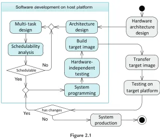
Figure 2.1
Real-time embedded systems development process.
As a road map,Figure 2.1shows the cross-development process for real-time embedded systems. At a high level, some activities need to be conducted on the host platform, while others need to be performed on the target platform. We next explain each of those activities.
2.2 Hardware Architecture
As far as embedded systems are concerned, a hardware architecture is an abstract
representation of an electronic or an electromechanical device that contains microprocessors, memory chips, and some peripherals (e.g., clocks, controllers, I/O devices, sensors, and actuators) as needed to fulfill its expected functionality.
Some common design factors related to hardware architecture design are as follows:
• Processing power.How fast a microprocessor will be required? A closely related factor is the processor’s power consumption, typically expressed in terms of millions of
instructions per second per milliwatt. A more powerful processor generally means higher power consumption, and a higher price too.
the evaluation board, and how much will be appropriate on the target system? A design with more memory on the evaluation board than what might be needed can often save a project that could have failed otherwise. However, more than necessary will certainly increase the production cost.
• Peripherals.What peripherals are required? Some advanced processor designs, also called microcontrollers or system-on-chip processors, have many built-in peripherals. Such a processor, if chosen, may be able to meet the needs for peripherals already. In general, it is advised to design a debugging interface (such as a serial port) on the evaluation board or the target system. When choices need to be made, performance always has higher priority than cost. A proven statement says that never use a $1.00 chip and expect the performance of a $10.00 chip.
• Reliability. Should the system be fail-proof? May it fail occasionally? What is the tolerable downtime?
• Future upgrade.How will field upgrades be performed?
We will learn some hardware fundamentals closely related to microprocessors and interrupts in Chapters 3 and 4, respectively.
2.3 Software Development
As shown inFigure 2.1, software development activities are performed on the host platform.
2.3.1 Software Design
Software design includes software architecture design, task design, and schedulability analysis:
• Software architecture design.How are different functional modules interrelated and synchronized? This topic is covered in Chapters 12 and 13.
• Task design.How many tasks should be considered? How should one assign priorities to those tasks? How should one document the task design and the timing constraints associated with the tasks? This is covered in Chapters 6–11 and 14.
• Schedulability analysis.As far as the identified timing constraints are concerned, is the set of tasks schedulable? This topic is covered in Chapters 15–17.
2.3.2 System Programming Language C/C++
utility called a compiler. This raises another requirement: a compiler has to be available for the chosen programming language such that the source code can be transformed into efficient binary code that is understandable to the processor selected in hardware design.
In practice, C and C++ are the de facto programming languages for embedded systems.1It is estimated that among all the embedded systems, about half of them are implemented in C, and about one third are implemented in C++. Their popularity is partially because C/C++
compilers are available for almost every processor type on the market.
The syntax of C/C++ programming is well beyond the scope of this book. Assuming the reader’s familiarity with C, we will learn in Chapters 18–23 a few implementation patterns that utilize some operating system kernel objects such as timers, semaphores, and message queues.
In the rest of this section, we briefly cover a few concepts (semantics) that are relevant to binary code generation.
1 //---start of a.h---extern int a;
3 static int sa=5;
//---end of
a.h---5
//---start of
b.h---7 int b(int p); static int sb=10;
9 //---end of
b.h---11 //---start of c.h---extern int c;
13 static int sc=3;
//---end of
c.h---15
//---start of
one.c---17 #include "a.h" #include "b.h" 19 int c = 2;
int main(void) 21 { int temp = 10;
sb = sb + temp;
23 printf("Invoke from %d: %d\n", a, sb); b(temp+sb);
25 sb = sb + temp;
printf("Invoke from %d: %d\n", a, sb);
27 b(temp+sb); return 0;
29 }
//---end of
one.c---31
//---start of
two.c---33 #include "c.h" #include "b.h" 35 int a = 1;
int b(int p2)
37 { static int temp = 2; sc++;
39 sb = sb + 2;
temp = p2+temp+sc+sb;
41 if (temp < 50) goto done; temp = 100;
43 done:
printf("Output from %d: %d\n", c, temp);
45 return temp; }
47 //---end of
two.c---Listing 2.1 An example C code.
A C/C++ program (application) can consist of numerous source files, each of which usually contains some#includedirectives that refer to header files. A compiler processes one source file at a time; it merges those headers with the source file to produce a transitory source file, which is called atranslation unitor a compilation unit.
InListing 2.1, there are two source files and three header files. The source file one.c together with a.h and b.h forms one translation unit, while the source file two.c together with b.h and c.h forms another translation unit.
2.3.2.1 Declarations and definitions
Each source or header file can define or declare many names, such as names for variables, names for functions, statement labels, tags for structures/unions/enumerations, identifiers for constants, and names for namespaces and classes in C++. The following discussion focuses on variable names and function names only.
We distinguish name declarations from name definitions. A name declaration simply states that the name belongs to the current translation unit. More than a name declaration, a name definition also imposes a requirement for storage.
declared in a.h; similarly the variablecis defined in one.c and declared in c.h. Note that the variabletempis defined, independently, in both functionsmain()andb(). The statement “extern int k = 0” is a definition of variablekbecause it has an initializer. • A function declaration is a statement containing a function prototype (function name,
return type, the types of parameters and their order). A function declaration is a function definition if the function prototype is also followed by a brace-enclosed body, which generates storage in the code space. For example, the functionb()in b.h is a function declaration, while the functionb()in two.c is a function definition.
A name declared in C/C++ may have attributes. For example, a variable name has a type, a scope, a storage duration, and a linkage; a function name has all those attributes except storage duration.
The type of a variable determines its size and memory address alignment, the values it can take, and the operations that can be performed on it. A function’s type specifies the function’s parameter list and return type.
We next examine scope, storage duration, and linkage in detail.
2.3.2.2 Scope regions
A name’s scope is that portion of a translation unit in which the name is visible. A name in an inner scope can hide a name from an outer scope. C and C++ each support five different kinds of scope regions [60]:
• File/namespace scope.In C, a name has file scope if it is declared in the outermost level of a translation unit. In C++, a name has namespace scope if it has file scope (global scope) or is declared in a namespace definition. InListing 2.1, names with file scope includea,b,
c,sa,sb,sc, andmain.
• Function scope.A statement label has function scope. A label can be defined only in the body of a function definition and is in scope everywhere in that body. InListing 2.1, the labeldonehas a function scope.
• Function prototype scope.A name has function prototype scope if it is declared in the function parameter list of a function declaration without a body. InListing 2.1, the parameterpof functionb()in b.h has function prototype scope.
• Block scope.A name has block scope (called local scope in C++) if it is declared within a function definition or a block nested therein. InListing 2.1, for the functionb()defined in two.c, the parameterp2and the variabletemphave block scope.
2.3.2.3 Storage duration
The storage duration of a variable determines the lifetime of the storage for that variable. Each variable in C/C++ has one of the following three storage durations:
• Static.For a variable with a static storage duration, its storage size and address are determined at compile time (before the program starts running); the lifetime of its storage is the entire program execution time. A variable declared at file/namespace scope has a static storage duration.
• Automatic.A local variable declared at block scope normally has an automatic storage duration. Local variables are stored in a run-time stack. Allocating storage for local variables usually takes just one machine instruction. Each time a function is called, a stack frame (a block of memory in the stack) is allocated for the function’s local variables, and the stack frame is deallocated when the function returns. Thus, for a variable with an automatic storage duration, the lifetime of its storage begins upon entry into the block immediately enclosing the object’s declaration and ends upon exit from the block. • Dynamic.A local variable declared at block scope can have a dynamic storage duration if
its storage is allocated by calling an allocation function, such asmalloc()in C or the operatornewin C++. Dynamic memory allocation allows a user to manage memory very economically. The drawback is that it is much slower than automatic allocation because it typically involves tens or hundreds of instructions. For a variable with a dynamic storage duration, the lifetime of its storage lasts until the memory is deallocated explicitly—say, by afreefunction in C or the operatordeletein C++.
2.3.2.4 Linkage
Linkage determines whether name declarations in different scopes can refer to the same name definition. The linkage attribute applies to both variable names and function names.
C and C++ support three levels of linkage:
• No linkage.A name defined in block scope or structure/class scope normally has no linkage. In such a case, it can be referenced by name only within its scope. Outside its scope, declarations of the same name refer to different entities. Function parameters and local variables normally have no linkage.
• Internal linkage.A name defined in file/namespace scope can have internal linkage. In such a case, it can be referenced by name only within the same translation unit. Outside the translation unit, declarations of the same name refer to different entities.
can be referenced from other translation units. Declarations of the same name always refer to the same entity. Global variables and functions normally have external linkage by default.
2.3.2.5 Storage-class specifiers
A variable declaration in C/C++ can be preceded by a storage-class specifier, which is used to change the way of creating the memory storage for the variable [61]. Both storage duration and linkage can be affected by the use of a storage-class specifier.
A storage-class specifier can be one of the following keywords:
• Auto.This specifier can be used only in declarations of local variables with block scope. All local variables in C/C++ are of the “auto” type by default, so the keyword “auto” is very rarely used explicitly. The “auto” specifier indicates a variable with an automatic storage duration. If it is uninitialized, such a variable has a garbage value.
• Register.This specifier can be used only in declarations of variables with block scope. The “register” specifier basically requests the compiler to store the variable in a register; this allows faster access than an “auto” variable, which is stored in the main memory. You are not allowed to take the address of a register variable. “Register” is the only storage-class specifier that can be used for function parameters.
• Extern.This specifier can be used in declarations of both variables and functions.
• A variable with the “extern” specifier has external linkage, which means that it can be referenced from other translation units. This also avoids unnecessary passing of variables as arguments during function calls.
• A variable with the “extern” specifier has a static storage duration, which means that its memory is allocated at compile time and it exists and retains its value as long as the program runs. If it is uninitialized, such a variable is set to 0.
• A local variable (block scope) normally has an automatic storage duration and no linkage. With the “extern” specifier, a local variable will have a static storage duration and external linkage.
• With or without the “extern” specifier, a global variable (file/namespace scope) by default has a static storage duration and external linkage.
• With or without the “extern” specifier, a function by default has external linkage, which means that it can be called from other translation units.
• Static.This specifier can be used in declarations of both variables and functions.
• A local variable (block scope) normally has an automatic storage duration. With the “static” specifier, a local variable will have a static storage duration. As a
consequence, its value persists between different function calls.2This will not affect its linkage (no linkage) and scope attributes.
• With the “static” specifier, a global variable (file/namespace scope) has its linkage attribute changed to “internal linkage.” For example, inListing 2.1, the global variable
sbdefined in b.h has a “static” specifier. The header b.h is included by both one.c and two.c. Although each of the two translation units uses the same namesb, it actually refers to a distinct entity in each translation unit.
• A function normally has external linkage. With the “static” specifier, a function will have internal linkage, which means that it may be called only within the translation unit in which it is defined.
By default, a local variable without a specifier is treated the same as one with “auto,” and a global variable without a specifier is treated the same as one with “extern” [62].
Table 2.1summarizes how a variable’s linkage and storage duration may be affected by a storage class specifier. Note that the only storage class specifiers allowed in a file/namespace scope declaration are “static” and “extern.”
Table 2.1 A variable’s linkage and storage duration depend on the storage class specifier
Storage Block Scope File/Namespace Scope Structure Member/Class Scope Class Linkage Storage Linkage Storage Linkage Storage
Specifier Duration Duration Duration
None No linkage Automatic Normally external linkage
Static No linkage Same as enclosing object
Auto No linkage Automatic NA NA NA NA
Register No linkage Automatic NA NA NA NA
Extern Normally external linkage
Static Normally external linkage
Static NA NA
Static No linkage Static Internal linkage Static External linkage in C++ only
Static in C++ only
NA, not applicable.
2.3.3 Test Hardware-Independent Modules
In practice, most modules of an embedded software are hardware independent. Hence, the skills for testing “general-purpose” software systems are equally applicable to the testing of those hardware-independent modules. For instance, test stubs, as used in the top-down testing approach, can be used to simulate the functionality of the software components that directly interact with hardware devices. As a simulator, a test stub of a module implements the interface of the actual module but simply providescanned responsesto calls made during testing.
The topic of testing is beyond the scope of this book, and the interested reader is referred to textbooks on testing such as [30, 31, 54, 55].
2.4 Build Target Images
In this section, we will look at the toolchain for building target images, and introduce a standard object file format—ELF. As a case study, we will also examine the image building process for embedded systems that rely on the QNX operating system.
2.4.1 Cross-Development Toolchain
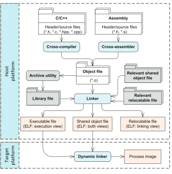
Figure 2.2shows the code transformation process involving a chain of cross-development tools: cross compiler/assembler, linker, and dynamic linker.
2.4.1.1 Cross compiler/assembler
A compiler is called anative compilerif its output is intended to directly run on the host platform (or the same type of environment) where the compiler runs. A cross compiler is a compiler capable of generating executable code for atarget platformthat is different from the host platform. This statement applies to a cross assembler as well, except that it processes source files written in assembly languages.
A cross compiler/assembler is useful in a number of situations:
• The target platform (e.g., an embedded system) has extremely limited resources. It is not powerful enough to run a native compiler to generate executable code by itself.
Figure 2.2
Cross-development toolchain.
For each compilation unit, the compiler/assembler generates an object file.3For instance, the C compiler can produce two object files—one.o and two.o—for the example code given in
Listing 2.1.
Each object file contains a symbol table. A symbol table is an array-like data structure consisting of entries about the global symbols (i.e., names of global variables and nonstatic functions) defined in the compilation unit, as well as the external symbols (with “external linkage”) referenced in the compilation unit. When the compiler encounters a symbol declaration, it stores that symbol and its attributes in the symbol table of the object file.4
3 The term “object” used in this context is different from the one used in object-oriented modeling/programming. 4 In object files, a symbol refers to a memory location, the content of which is either data for a variable or code for
For the example code given inListing 2.1, we have the following:
• In one.c, there are four global symbol definitions: global variablesc,sa, andsb, and a functionmain(). It references two external symbolsaandb().
• In two.c, there are four global symbol definitions: global variablesa,sb, andsc, and a functionb(). It references the external symbolc. The symbol table also has an entry for
temp, which is a local variable with a static storage duration.
An object file’s symbol table holds information that is needed by a compiler/linker to locate and relocate a program’s symbolic definitions and references.
2.4.1.2 Linker
A complete program (application) is typically composed of multiple object files, each of which may cross-reference the definitions for data or functions defined in the other object files. The process of combining multiple object files into a single object file is called static linking, which is performed by a computer program known as a linker or link editor. The compiler automatically invokes the linker as the last step of compiling.
A linker has two major jobs:
1. Symbol resolution.While a linker is processing the application-specific object files, it needs to analyze each object file and determine where symbols with external linkage are defined. External symbol references may also involve application-independent object files—those that define commonly used functions (say,printf) for a wide range of applications (some known as archived library files, some known as .so, or sharable object files). It is worth noting that two variables of the same name can be defined in different scopes. InListing 2.1, a static variablesbis defined in both one.c and two.c. This will not confuse the linker because the compiler has treated them as distinct symbols. Essentially the compiler uses “namespace” to distinguish variables: a local variable name is tagged by the function to which it belongs and a global variable name is tagged by the file name. 2. Symbol relocation.The final object file produced by a linker contains all the symbol
definitions originating from the input object files, as well as those from static library files. As the linker merges the input object files and inserts code from the library files, the symbol offsets are changed. By symbol relocation, the linker, via a relocation table, modifies the binary code of the final object file so that each symbol reference reflects the actual address assigned to that symbol.
A linker can generate three types of object files: relocatable file, executable file, and shared object file:
• Executable file.An executable file holds code and data suitable for execution. In an operating system, the basic unit of execution is called a process orprocess image, which is dynamically created from an executable file (say, as a result of an exec or spawn call). For systems supporting virtual memory, each process is put into its own address space. • Shared object file.A shared object file holds code and data suitable for further linking. It
can be combined with other relocatable and shared object files to create another object file. Some shared object files aredynamically linkable, and are intended to be loaded at run time and can be simultaneously shared by multiple process images.
2.4.1.3 Dynamic linker
In order to create a process image for an object file, the object file has to be loaded from its storage location into RAM. This job is performed by a program interpreter, which
• itself is an executable file or a shared object file;
• is self-interpreted (it does not need another program interpreter);
• is able to receive control from the system and provide a running environment for the object being loaded.
Aprogram loaderis a program interpreter that simply loads a program into memory and transfers the execution control to it. This approach works for stand-alone executable files. An executable file is stand-alone when it contains one copy for each library routine used in the program. This makes the executable object easier to distribute to diverse target environments, at the cost of larger memory space.
Another type of program, instead of having an embedded copy for each library routine, contains only reference information of sharable library routines. Obviously, such a program requires the presence of library files on the target system. It also demands adynamic linker—a program interpreter that is more powerful than a simple program loader. A dynamic linker, once it has gained control from the system, will first load the whole program into memory to form an initial process image, then resolve symbolic references dynamically by loading and binding external shared libraries to form a complete process image, and finally transfer control to the process. This procedure is also called dynamic linking.
An advantage of dynamic linking is that multiple applications can share a single copy of a library. This also implies that a deployed system can automatically benefit from bug fixes and upgrades to libraries.
2.4.2 Executable and Linking Format
adopted object file format.5It supports cross-compilation, initializer/finalizer (e.g., the constructor and destructor in C++), dynamic linking, and other advanced system features.
An ELF object file has an ELF header, a section header table and/or a program header table, and a series of sections or segments. As shown inFigure 2.3, the ELF header of an object file resides at the beginning; it serves as a “road map” for the rest of the object file. An ELF header has the following fields:
• The first four bytes mark the file as an ELF object file. The “class” byte can take a value of 1 or 2, indicating the support for 32-bit or 64-bit processor architectures, respectively. The “data” byte can take a value of 1 or 2, specifying ELFDATA2LSB or ELFDATA2MSB as the data-encoding format. The encoding ELFDATA2LSB specifies 2’s complement values,6with the least significant byte occupying the lowest address. The encoding ELFDATA2MSB specifies 2’s complement values, with the most significant byte occupying the lowest address. The “pad” bytes are unused and are reserved for future changes.
• The “type” field indicates the object file type, which can take a value of 1, 2, or 3, representing relocatable file, executable file, or shared object file, respectively.
• The “machine” field specifies the required architecture for this object file. For example, the value 3 is reserved for Intel 80386 processors, and 40 is reserved for ARM processors. • The “version” field identifies the version of the object file format, which is fixed to 1 for
the current standard.
• The “entry” field gives the memory address of an entry point to which the system first transfers control. A system may have many entry points—say, for reset, interrupts, and software interrupts. However, an executable file can have one and only one entry point. • The “phoff” field holds the byte offset of the program header table in the object file. It is
zero if the file has no program header table.
• The “shoff” field holds the byte offset of the section header table in the object file. It is zero if the file has no section header table.
• The “flags” field holds processor-specific flags associated with the file. It is zero for the 32-bit Intel architecture because it defines no flags.
• The “ehsize” field holds the ELF header’s size in bytes.
• The “phentsize” field holds the size in bytes of one entry in the file’s program header table; all entries are of the same size.
• The “phnum” field holds the number of entries in the program header table.
5 Another standard format is named common object file format (COFF).
6 In a 2’s-complement binary number representation, the weight of each bit is a power of 2, except for the most
• The “shentsize” field holds the size in bytes of one entry in the file’s section header table; all entries (section headers) are of the same size.
• The “shnum” field holds the number of entries in the section header table.
• The “shstrndx” field holds an index in the section header table, giving the entry associated with thesection-header string table.
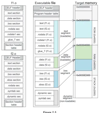
The ELF standard provides two parallel views of an object file’s contents. On the one hand, an ELF object file can be viewed asa series of named sections. This “linking” view is taken by compilers/assemblers and linkers. Sections are intended for further processing by a linker. On the other hand, an ELF object file can be viewed asa series of named segments. Segments are intended to be mapped into memory to create a process image. This “execution” view is taken by dynamic linkers or program loaders.
2.4.2.1 Linking view
Figure 2.3shows the linking view of ELF, where it is optional to have a program header table. For example, there is no program header table in a relocatable file, whereas a shared object file may or may not have a program header table.
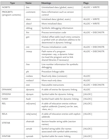
Table 2.2lists some default sections with predefined names. Each section contains a single type of information, such as program code (instructions), data, symbol, or relocation information. Typically, an object file may have
• a .text section for executable instructions; • a .data section for initialized data;
• a .bss (for “block started by symbols”) section for uninitialized data; • a .symtab section (symbol table) for static linking;
n
n
j
Table 2.2 Some predefined section headers, their types, and their attributes
Type Name Meanings Flags
NOBITS .bss Uninitialized data (global, static) ALLOC + WRITE
PROGBITS .comment Extra information such as version (program contents) control
.data Initialized data (global, static) ALLOC + WRITE
.data1 More initialized data ALLOC + WRITE
.debug Symbolic debugging information
.fini Process termination code ALLOC + EXECINSTR
.got Global offset table (each entry contains a symbol with an absolute address to be determined in dynamic linking)
.init Process initialization code ALLOC + EXECINSTR
.interp Path name of a program interpreter—say, a dynamic linker (to load the program and to link shared libraries if necessary)
ALLOC + EXECINSTR
.line Line number information for symbolic debugging
.plt Procedure linkage table
.rodata Read-only data (constant) ALLOC
.rodata1 More read-only data ALLOC
.text Executable instructions ALLOC + EXECINSTR
DYNAMIC .dynamic A table of entries for dynamic linking ALLOC
DYNSYM .dynsym Symbol table for dynamic linking [ALLOC]
HASH .hash Symbol hash table for dynamic linking [ALLOC]
REL .rel[name] A table of relocation entries without explicit addends ([name] can be .text, .data, etc.)
[ALLOC]
RELA .rela[name] A table of relocation entries with explicit addends
[ALLOC]
STRTAB .shstrtab Section-header string table (section names)
.strtab Symbol string table (for names associated with symbol table entries)
[ALLOC]
• a .strtab section holding a symbol string table;
• a .shstrtab section holding a section-header string table; and
• a few .rel[name] sections each containing the relocation information for a specific section with the name [name].
Each section in an object file occupies one contiguous (possibly empty) sequence of bytes, and has exactly one section header describing it. A section header has the following fields:
• The “name” field specifies the name of the section. Its value is an index in the .shstrtab section (section-header string table), giving the location of a null-terminated string. • The “type” field categorizes the section’s contents. The first column ofTable 2.2lists
some of the supported types.
• The “flags” field supports one-bit flags: 0x1 for WRITE (the section contains writable data), 0x2 for ALLOC (the section occupies memory during process execution), and 0x4 for EXECINSTR (the section contains executable machine instructions).
• The “addr” field, if not zero, gives theload address7; that is, the starting address in the NVM at which the section’s first byte resides.
• The “offset” field gives the byte offset from the beginning of the file to the first byte in the section.
• The “size” field gives the section’s size in bytes.
• The “link” field, for a section related to dynamic linking or relocation, holds a section header index of a string table or symbol table.
• The “info” field, for a .rel or .rela section, holds the section header index of the section to which the relocation applies.
• The “addralign” field holds a value of 0 or positive integral powers of 2, specifying a constraint for section address alignment. If the value of addralign is greater than 1, the value of addr must be congruent to 0, modulo the value of addralign.
• The “entsize” field, if not zero, gives the size in bytes of an entry of a table section.
2.4.2.2 Execution view
Figure 2.4shows the execution view of ELF, where it is optional to have a section header table. In this view, an object file is a set of segments described by a program header table, which is meaningful only for executable and sh