IRT in Item Banking, Study of DIF Items and Test Construction : Item Response Theory in Item Banking, Study of Differentially Functioning Items and Test Construction

Master Thesis

IRT in Item Banking, Study of DIF Items and Test Construction

(Item Response Theory in Item Banking, Study of Differentially Functioning Items and Test Construction)

Gembo Tshering

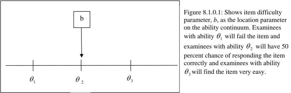
s0129836

M.Sc Student

Master of Science-Track Educational Evaluation and Assessment

Educational Science and Technology

Master Thesis

IRT in Item Banking, Study of DIF Items and Test Construction

(Item Response Theory in Item Banking, Study of Differentially Functioning Items and Test Construction)

Supervisors

First Mentor

Dr. Bernard P. Veldkamp University of Twente

(Assistant

Professor)

Second Mentor

Dr. Hans J. Vos University of Twente

(Assistant

Professor)

External Mentor

Dr. Bas T. Hemker National Institute of Educational Measurement, CITO

(Psychometrician)

Bhutan Board of Examinations

Ministry of Education

Royal Government of Bhutan

Bhutan

Netherlands Fellowship Programmes

Netherlands Organization for International Cooperation in

Higher Education (NUFFIC)

Ministry of Education, Culture and Science

The Netherlands

University of Twente

Educational Science and Technology

The Netherlands

CITO

National Institute of Educational Measurement

The Netherlands

This page is dedicated to the above organizations for giving me

an opportunity to develop academically and acquire the capacity

to interact with knowledge and wisdom available within the vast

Preface

Classical Test Theory (CTT) had been a sole principle of measurement for the measurement specialists until 1970s. In the decades of the 1970s, Item Response Theory (IRT) began to pick up momentum among the measurement specialists. The weaknesses inherent in CTT are readily redressed by IRT. However, CTT is still used by the measurement specialists due to its simplicity compared to IRT in terms of both mathematical complexity and requirement of special computer packages. Where expertise and special computer packages are available, IRT is always a first choice. The existence of local independence and invariance of item parameters across examinee groups makes IRT superior to CTT. The limitations due to lack of adequate statistics for studying differential item functioning and item bias and incapability of producing tailored tests naturally make CTT inferior to IRT. CTT upsets the measurement specialists when they are confronted with the task of building item banks. The item parameters obtained by using CTT change when the group of examinees changes. For instance, the items are easy when examinees are able and items are difficult when examinees are not able, meaning that the difficulty of the ability being measured change as the examinees change. This is undesirable because ability should maintain its level of complexity irrespective of where, how, when and who are tested on it. Item banking is often used as a quick and efficient means to test as and when desired and this requires the items in the item bank to measure the abilities they are supposed to measure with the same level of complexity across different examinations. Once again CTT fails to serve the measurement specialists in dealing with item banking.

Despite the complexity of expertise involved in it, IRT is widely applied in making paper and pencil tests, studying differential item functioning , item banking and computer adaptive testing (CAT). I have been very lucky to have the opportunity to put the principles of CTT and IRT into practice through a project at the National Institute of Educational Measurement, CITO, Arnhem, the Netherlands.

The project pet named as Using Item Bank in making Tests for English Reading and Vocabulary

Constructs (UIBTERV) is contracted to me by CITO through contract award reference number

2006-HRM-037. It has been a very challenging, exciting and above all extremely motivating throughout the course of the project execution. Learning One-Parameter Logistic Model (OPLM), using OPLM to calibrate items, studying differential item functioning with OPLM, producing high stake test for the 1st year students of the Dutch Lower Secondary Education with OPLM, calibrating items for the item bank with OPLM and extending item bank with new items have given me the first hand experience with the use of CTT and IRT in the field of measurement.

However all these invaluable experiences have come to me not without the involvement of prominent personalities from the University of Twente, Educational Science and Technology, Enschede, the Netherlands and the National Institute of Educational Measurement, CITO, Arnhem, the Netherlands. Dr. Bernard Veldkamp from the University of Twente introduced CITO to me while attending one of his classes from the course on Designing Educational Assessment. With his keen interest in my desire, enthusiasm and determination to have a first hand knowledge of CTT and IRT, introduced me to CITO and soon afterwards we made a couple of trips to CITO to look for a project.

Dr. Bernard Veldkamp has supported my work on the thesis right from the beginning to the end by reading the draft chapters as and when I was able to put them up for his kind attention. He also read the complete draft thesis. The occasions always resulted into valuable comments and feedback.

Ms Angela Verschoor is an expert in CAT, but I soon learned that I would not have a share of knowledge from her only because UIBTERV is a paper and pencil tests project. Dr. Bas Hemker is a psychometrician at CITO and UIBTERV is one of his projects. Dr. Bas Hemker not only spared UIBTERV for me, but he also consented to be my external supervisor at CITO who is due to be involved almost daily with me on UIBTERV. It is with constant maneuvering and guidance from Dr. Bas Hemker that I discovered what I have been looking for in UIBTERV and made my work a success.

Dr. Bas Hemker led me to a couple of meetings on entrance test for English Reading Comprehension and Vocabulary test with test experts Ms. Marion Feddema and Ms. Noud van Zuijlen, where I learnt how the test statistics are used for making decision about the prospective examinees.

OPLM, item calibration, study of differential item functioning, test construction and extending item bank have been continuous lessons imparted to me by Dr. Bas as I ploughed through UIBTERV. Indeed, it is his continuous support, interest and confidence in my progress with UIBTERV that I realized I could complete the project as per the deadline set in the contract.

I also continuously enjoyed the goodwill of CITO through other personalities. “A theoretical knowledge is never as beautiful as a practical knowledge” is a comment from Prof. Dr. Piet Sanders, Head of the Department of Psychometrics, CITO, which echoed continuously and triggered a daily quest that I would claim as a realization at the end of a hard day work. Dr. Timo Bechger’s demonstration of Newton Raphson Estimation procedure as used for MML estimation with MathCad is a pleasure hard to forget.

My friends Mr. Wouter Toonen, and Dr. Huseyin Yildrem have been wonderful friends. Although, each one of us was always conscience stricken by fast evading time, we would occasionally manage to turn around and laugh over small talks.

Last but not least, I would have been extraordinarily forgetful if I did not mention my association with the second mentor DR. Hans Vos. Dr. Hans Vos has been a constant source of inspiration to me. His interest in me led me to an additional experimental success at CITO through conducting an experiment on Standard Setting by using Bookmark method in collaboration with Dr. Maarten de Groot, psychometrician. Dr. Hans Vos has read the complete thesis and I once again say thank you to him for his valuable feedback and comments.

Finally I would like to thank everyone who has been a part of this thesis. My thanks are due to (a) NUFFIC for sponsoring me the master of science (M.Sc) degree course vide fellowship award letter NFP-MA.05/1518\GW.07.05.250/fl\file number 022/05\dated June 9, 2006, (b) University of Twente, Educational Science and Technology for being home and family abroad while pursuing M.Sc. and (d) National Institute of Educational Measurements, CITO, for contracting the project and also sponsoring my daily involvement in it.

Gembo Tshering Educational Science and Technology University of Twente Enschede The Netherlands

Contents

Page

Preface

……….

iv

Chapter

Using Item Bank in making Tests for English Reading and

Vocabulary Constructs

………..

1-7

1.0.0 Introduction………

1

1.1.0

Dutch Education System……… 1

1.1.1

Student Monitoring System………... 2

1.2.0 UIBTERV……….

3

1.2.1 UIBTERV

Data……….

4

1.2.2

Problems in UIBTERV……….. 5

1.2.3

Goals of UIBTERV………... 6

1.3.0

Chapters in the Thesis……… 6

1.3.1 Summary………

7

1

1.3.2 References………..

7

A Review of Classical Test Theory

………

8-17

2.0.0 Introduction………

8

2.1.0

Classical Test Theory……….... 8

2.2.0

Assumptions of Classical True Score Theory…………... 8

2.2.1 Assumption

1………...

8

2.2.2 Assumption

2………...

8

2.2.3 Assumption

3………...

9

2.2.4 Assumption

4………...

9

2.2.5 Assumption

5………...

9

2.2.6 Assumption

6………...

9

2.2.7 Assumption

7………...

9

2.3.0 Test

Reliability………...

10

2.3.1

Different ways of Interpreting the Reliability Coefficient

of a Test……….

10

2.3.2

Use of the Reliability Coefficient in Interpreting Test

Scores……….

11

2.4.0

Two popular Formulae for Estimating Reliability……... 12

2.4.1 Internal-Consistency

Reliability………...

12

2.4.2

The Spearman-Brown Formula………. 12

2.5.0

Standard Errors of Measurement and Confidence

Intervals……….

13

2.6.0 Validity………..

14

2.6.1 Content

Validity………...

14

2.6.2 Criterion

Validity………...

15

2.6.3

Reliability of Predictor and Criterion Validity………….. 16

2.6.4 Construct

Validity………..

16

2.7.0 Summary………

17

3

Item Parameters in CTT Context

……….

18-24

3.0.0 Introduction………

18

3.1.0 Item

Difficulty………...

18

3.1.1

Role of P-values in Item Analysis………. 19

3.2.0 Item

Variance……….

19

3.2.1

Role of Item Variance in Item Analysis……… 20

3.3.0 Item

Discrimination………...

20

3.3.1

Index of item Discrimination………. 20

3.3.1.1

Role of Index of Discrimination in Item Analysis………. 20

3.3.2

Point Biserial Correlation……….. 20

3.3.2.1

Role of Point Biserial in Item analysis……….. 21

3.3.3

Biserial Correlation Coefficient………. 21

3.3.3.1

Role of Biserial Correlation Coefficient in Item Analysis 21

3.4.0 Item

Reliability

Index………

21

3.4.0.1

Role of Item Reliability Index in Item Analysis………… 22

3.5.0

Item Validity Index……… 22

3.5.0.1

Role of Item Validity Index in Item Analysis…………... 22

3.6.0

Making Test from Item Bank……… 22

3.7.0 Summary………

22

3.8.0 References………..

24

Making Norm Reference Table

……….

25-27

4.0.0 Introduction………

25

4.1.0 Norming

Study………...

25

4.2.0

Making Norm Table……….. 25

4.3.0 Percentile

Rank………..

26

4.4.0 Summary………

26

4

4.5.0 References………..

27

Item Response Theory

………

28-30

5.0.0 Introduction………

28

5.1.0

Item Response Theory………... 28

5.2.0

Assumptions of Item Response Theory………. 28

5.2.1

Dimensionality of Latent Space………. 28

5.2.2 Local

Independence………...

29

5.2.3

Item Characteristic Curves……… 29

5.2.4 Speededness………...

30

5.3.0 Summary………

30

5

5.3.1 References………..

30

6

One-Parameter Logistic Model (OPLM)

……….

31-40

6.0.0 Introduction………

31

6.1.0

Presentation of One-Parameter Logistic Model………… 31

6.2.1 The

M

i

Tests……….. 32

6.2.2 The

S

i

Tests……… 33

6.2.3 The

R1

c

Tests………. 34

6.3.0 Parameter

Estimation……….

36

6.3.1

Conditional Maximum Likelihood Estimation………….. 36

6.3.2

Marginal Maximum Likelihood Estimation……….. 37

6.4.0

OPLM and other Models………... 37

6.4.1

OPLM and Rasch Model………... 37

6.4.2

OPLM and Two-Parameter Logistic Model……….. 37

6.4.3

OPLM and Partial Credit Model……… 38

6.4.4

OPLM and Generalized Partial Credit Model…………... 38

6.5.0 Strengths

of

OPLM………

38

6.6.0 Summary………

39

6.7.0 References……….

39

Item and Test Information Functions

………..

41-44

7.0.0 Introduction………

41

7.1.0

Item Information Function for Dichotomous Model……. 41

7.2.0

Test Information for Dichotomous Model………

41

7.3.0

Item Information Function for Polytomous Model……... 42

7.4.0

Test Information Function for Polytomous Model……… 42

7.5.0

Test Information Function and Standard Error of

Measurement……….

43

7.6.0 Summary………

44

7

7.7.0 References………..

44

Item Calibration

……….

45-56

8.0.0 Introduction………

45

8.1.0

Type of IRT Model used for Item Calibration…………... 45

8.2.0

Steps of Item Calibration………... 46

8.2.1

Fitting OPLM to UIBTERV Data……….

46

8.2.2 Analysis

1………..

47

8.2.3

Analysis 2: Goodness of Fit Test………... 47

8.3.0

Analysis 3: Differential Item Functioning………. 48

8.3.1

Gender DIF Analysis………. 50

8.3.2

School Level DIF Analysis……… 52

8.4.0 Summary………

56

8

8.5.0 References………..

56

Generating Item Information and Global Norms

………...

57-63

9.0.0 Introduction………

57

9.1.0 Global

Norm………..

57

9.1.1 Population

Parameters………...

57

9.1.2

Estimation of Population Parameters………

57

9.1.4

Interpreting Global Norm Table and Moments of

Distribution………

59

9.2.0 Item

Information………

60

9.3.0 Summary………

63

9.4.0 References………..

63

Making English Reading Comprehension Entrance Test

…………..

64-71

10.0.0 Introduction………

64

10.1.0

Assembling Tests from Item Pool………. 64

10.1.1 Specifying

Ability

Range………..

64

10.2.0

Making Norm Reference Table for Tests……….. 66

10.3.0

Norm Reference Table for 3 versions of Test…………... 67

10

10.4.0 Summary………

71

Item Banking and Linking New Items to Old Item Bank

…………..

72-86

11.0.0 Introduction………

72

11.1.0

Item Bank and its Functions……….. 72

11.2.0

Building Item Bank……… 72

11.2.1

Calibrating Items from Different Tests on Common

Scale………...

73

11.2.2

Replenishing Item Bank……… 73

11.2.3

Mean and Sigma Method of Determing Scaling

Constants………

74

11.2.4 OPLM Method of Linking Items ………..

80

11.2.4.1 Method I……….

81

11.2.4.2 Method II………

81

11.2.5 Comparison of Mean and Sigma and OPLM methods of Linking Items……….

84

11.2.6 Summary………

86

11

11.2.7 References………..

86

Discussions and Future Developments………

87-88

12.0.0 Introduction………

87

12.1.0 Discussions……….

87

12.2.0 Future Developments………...

88

12

12.3.0 Summary………

88

Appendix I

Global Norm Table for UIBTERV English Reading Comprehension Test

Chapter 1

Using Item Bank in making Tests for English Reading and Vocabulary Constructs

1.0.0 Introduction

The project Using Item Bank in making Tests for English Reading and Vocabulary (UIBTERV) consists of a series of continuous stage by stage tasks. The stages that UIBTERV went through were (a) writing test items for English reading and vocabulary constructs for Lower Secondary Education of the Netherlands, (b) assembling the test items into thirteen test booklets with each booklet containing seventy tests items, (c) pre-testing the test booklets with sample schools, (d) correction and scoring of the pretested booklets and (e) construction of data banks for the scores obtained from the pretests. My role in UIBTERV begins from the last stage, i.e., stage e. Although my role begins somewhere from the middle and will end somewhere short of touching the end of UIBTERV, it is important to understand UIBTERV from its holistic perspective to have an idea of an immensity of stake it carries against thousands of Dutch students.

In this chapter, a brief description of the Dutch education system will be presented and UIBTERV will be described in terms of its goals, current situation and future line of plans in the light of Dutch Secondary Education. Finally, this chapter will complete with short tour of the subsequent chapters.

1.1.0 The Dutch Education System

The education system of the Netherlands is composed of different levels. The different levels are Primary Education, Special Primary Education, Lower Secondary Education, Pre- University Education, Senior General Secondary Education, Pre-Vocational Secondary Education, Vocational Training Programme, Special Secondary Schools, University Education, Higher Professional Education, and Senior Secondary Vocational Education. The relationships among the different levels and the direction of movements form one level to another level are displayed in figure 1.1.0.1 (CITO, 2005, p.7).

The Primary Education in the Netherlands spans a duration of eight years. The children are allowed to begin school at the age of four and they are legally obliged to be in the schools at the age of five. Of the eight years, the last seven years are compulsory. When the children graduate from the Primary Education, they are given a recommendation on the type of secondary education that they should pursue. The recommendation is based on the results of the four different kinds of tests conducted in four areas, viz., (a) language, (b) arithmetic/mathematics, (c) study skills and (d) world orientation. The teachers also play very important role in enhancing the validity of the recommendation by providing additional information about their students. The Primary Education has also Special Primary Education for the students with learning and behavioral problems.

The VWO curriculum prepares students for research oriented university education, the HAVO curriculum prepares them for professional university education and the Pre-Vocational Secondary Education curriculum prepares them for Senior Secondary Vocational Education.

1.1.1 Student Monitoring System

The movements of students from Primary Education to Secondary Education and the types of schooling they will pursue are monitored by the Student Monitoring System. Generally the Student Monitoring System is implemented in Primary Education and in Secondary Education. The professional body responsible for developing, managing, executing and reporting the matters relevant to the Student Monitoring Systems is the National Institute of Educational Measurement, CITO, located at Arnhem in the Netherlands. The National Institute of Educational Measurement does everything concerning educational assessment, measurement and evaluation in the Netherlands and to a certain extent its expertise sail abroad as well. The readers may like to visit www.cito.com for more discoveries and information about the National Institute of Educational Measurement, CITO, Arnhem, the Netherlands.

The Student Monitoring System is highly psychometric based on quantitative research with elements of longitudinal design. At both Primary Education and Secondary Education levels, the Student Monitoring System consists of entrance tests, follow-up tests and advisory tests. The contents of the

Figure 1.1.0.1: The Dutch Education System

University (WO)

Higher Professional

Education (HBO)

Senior Secondary Vocational Education

Pre-University

Education (VWO)

Senior General Secondary Education

(HAVO)

Pre-vocational Secondary

Education

Vocational

Training

Programme

(BB+)

Lower Secondary Education

Special Secondary

Schools

Primary Education

Education

Special P

rimary

Education

Age 4

Age 18

Age 12

The Dutch Education System

6 5 4 3

2 1

8 7 6 5 4 3 2

Compulsory Education

1

VWO HAVO GT KB BB BB+

Year

student monitoring systems are different for Primary Education and Secondary Education because they have structural differences. The Student Monitoring System of Primary Education is not within the scope of the thesis and also the scope of the thesis does not warrant a detailed description of the Student Monitoring System of the Secondary Education. In case of the Student Monitoring System of the Secondary Education, a detailed description of the role of the Department of Psychometrics at CITO in producing entrance tests, follow-up tests and advisory tests will be presented throughout the thesis.

The Student Monitoring System of the Secondary Education seeks to 1. measure an individual student’s competence.

2. measure student’s competence relative to the fellow students. 3. measure the progress of an individual student.

4. measure the progress of a student with reference to the fellow students.

5. advise student on the choice of the types of schools he/she could pursue in the third year of the Secondary Education.

The five goals of the Student Monitoring System of the Secondary Education link students with teachers by presenting answers to the following questions:

• How much progress is made by my students?

• Is the progress made by my students sufficient?

• Is there a standstill or deterioration in the students’ development and what can I do about it as a teacher?

• Is the subject matter offered by me as a teacher adequately geared to the level of the students?

• Which student needs extra help and attention?

• Do I have to address or change my didactic approach as a teacher?

• Are there any parts of the educational programme in need of improvement?

• What are the positions of my students with respect to the students of other classes and the students of other schools?

To achieve the five goals and to get answers to the questions, the Student Monitoring System of the Secondary Education uses three tests, viz., (a) entrance tests, (b) follow-up tests and (c) advisory tests. In a nutshell, the School Monitoring System purports to (a) help teachers monitor their students’ development, (b) provide tools to help students decide on the type of schooling they should choose after successfully completing the Lower Secondary Education and (c) monitor the quality of the educational process. UIBTERV has direct relevance to the Student Monitoring System of the Secondary Education.

1.2.0 UIBTERV

Three Tests Test Area _Entrance

Test

Test after 1st Year

Test after 2nd Year Dutch Reading Comprehension Prepared Prepared Prepared English Reading Comprehension UIBTERV Prepared Prepared Mathematics Prepared Prepared Prepared Study Skills Prepared Prepared Prepared Table1.2.0.1: Shows test areas and types of tests offered by The Student Monitoring System.

In table 1.2.0.1, prepared indicates that the tests were ready for administration. Where UIBTERV is concerned, the tests are to be prepared. Each test in table 1.2.0.1 has three versions corresponding to three difficulty levels. For instance, an entrance test in English Reading Comprehension has three different tests of three different difficulty levels, viz., (a) an Easy and Average Easy Test, (b) an Average Easy and Average Difficult Test and (c) an Average Difficult and Difficult Test. Table 1.2.0.2 shows this relationship.

The combination of (a) easy items and average easy items makes up an Easy and Average Easy Test for the students studying in BB+/BB section of the Secondary Education, (b) average easy items and average difficult items makes up an Average Easy and Average Difficult Test for the students studying in KB/GT section of the Secondary Education and (c) average difficult items and difficult items makes up an Average Difficult and Difficult Test for the students studying in HAVO/VWO section of the Secondary Education.

The three versions of the test are overlapped by using common items. The test for BB+/BB and the test for KB/GL are overlapped by using average easy items as the common items. The test for KB/GT and the test for HAVO/VWO are overlapped by using average difficult items as the common items. The common items link the three versions of the test which is a necessary condition to place them on a common scale for comparative studies of their results.

Entrance Test Target Population

Easy Average Easy Average Difficult Difficult BB+/BB

KB/GT HAVO/VWO

Table 1.2.0.2: Shows how Entrance Test is divided into three tests for three levels of secondary education.

1.2.1 UIBTERV Data

The test booklets were administered to 1280 students. The data are joined in a complete dataset. A portion of data from the data file EngEntNw.DAT is shown in table 1.2.1.1.

19828 2218 01 J 19085 0 0 39 1 1 1 1 1001100010111001101110010010101111101011101101100101010100101100111010 19828 2220 01 J 08045 1 0 51 1 1 1 1 1110110010011111111101011011111101111110111101110100111100100111111110 19828 2190 01 J 06125 1 0 59 1 1 1 1 1111110011011011111111011111111111111100111101110111101111111101111111 19828 2189 01 J 09046 1 0 62 1 1 1 1 1111110111011111111111111110111101111110111111110111111101111101111111 . . .

. . . . . . . . .

30442 0163 02 J 07024 6 0 45 2 2 2 2 0000110111000111001011110110100001011101111111111101111010101110101111 22906 0096 02 J 25066 1 0 53 2 2 2 2 1101100111010110101111101111111101011101101110111111101011011110111111 30442 0166 02 J 21025 1 0 56 2 2 2 2 1110101110110101111111111111101110111111111110111100110110111101111110 22906 0093 02 J 29115 1 0 51 2 2 2 2 1111101000100111010111111111101110011111011110101101111011001110111111 . . .

. . . . . .

30442 0161 02 J 18074 5 0 62 2 2 2 2 1111111101111111011111111110110110011111111111111110110111111111111111 22906 0095 02 J 05016 1 0 59 2 2 2 2 1111111110110111111111111111110111011111111110111101101010111100111111 30442 0162 02 M 03035 3 0 36 2 2 2 15 0110000100100110110011010111100011011110101110001000101011001111001010

Table 1.2.1.1: Excerpts from UIBTERV data file EngEntNw.DAT.

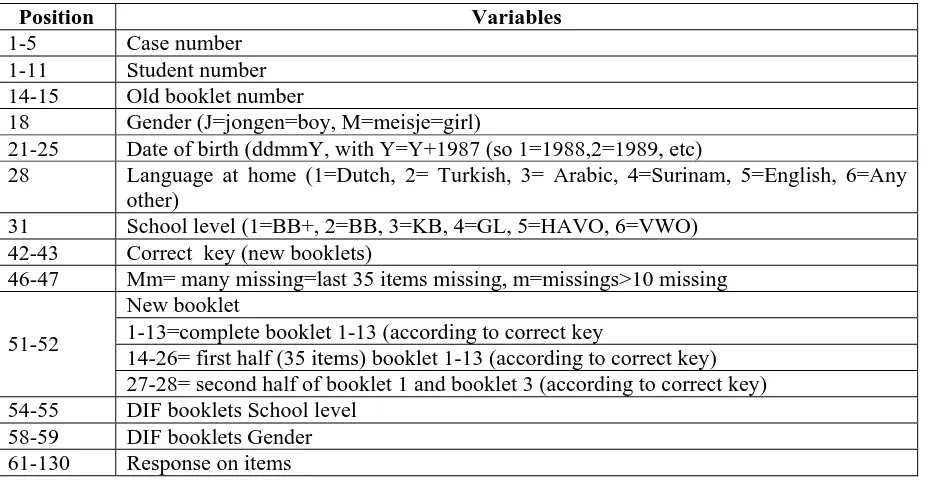
The data has the following variables with the positions specified against them:

Position Variables

1-5 Case number 1-11 Student number 14-15 Old booklet number

18 Gender (J=jongen=boy, M=meisje=girl)

21-25 Date of birth (ddmmY, with Y=Y+1987 (so 1=1988,2=1989, etc)

28 Language at home (1=Dutch, 2= Turkish, 3= Arabic, 4=Surinam, 5=English, 6=Any other)

31 School level (1=BB+, 2=BB, 3=KB, 4=GL, 5=HAVO, 6=VWO) 42-43 Correct key (new booklets)

46-47 Mm= many missing=last 35 items missing, m=missings>10 missing New booklet

1-13=complete booklet 1-13 (according to correct key

14-26= first half (35 items) booklet 1-13 (according to correct key) 51-52

27-28= second half of booklet 1 and booklet 3 (according to correct key) 54-55 DIF booklets School level

58-59 DIF booklets Gender 61-130 Response on items

Table 1.2.1.2: Variables and their positions.

1.2.2 Problems in UIBTERV

A Follow-Up Test and an Advisory Test in English Reading Comprehension are ready for administration. An Entrance Test in English Reading Comprehension and Vocabulary is due to be prepared from the pretested test booklets and the unused items have to be banked for future use in assembling similar tests. The situation elevates a platform to delineate problems in UIBTERV.

The first challenge is to calibrate the pretested items from the thirteen test booklets, each test booklet having 70 test items with some anchor items. The anchor items relate the items from different booklets to each other and make them comparable. The second challenge is to assemble entrance tests for Secondary Education for three populations, as shown in figure 1.2.0.2. The third challenge is to develop norm tables for the entrance tests. The fourth challenge is to successfully link the new items to the old item bank. The old item bank has the items from the Follow-Up Tests and the Advisory Tests on English Reading Comprehension and Vocabulary.

By linking items from Entrance Tests with other items available in the old item bank, the items will be placed on the common scale which will make the comparative study of the results from three tests on English Reading Comprehension and Vocabulary possible. The comparative study across all three tests will make the monitoring of student’s learning progress possible.

1.2.3 Goals of UIBTERV

The goals of UIBTERV are to

(1) prepare test specifications. (2) prepare item pool. (3) field test the items.

(4) calibrate the field tested items. (5) develop global norm.

(6) assemble test items. (7) develop local norms.

(8) extend the old item bank by adding items from the field tested items. (9) publish entrance test for lower secondary education.

The goals 1, 2 and 3 were successfully completed before I took up UIBTERV and goal 9 is beyond the scope of my contract with CITO, Arnhem, the Netherlands. Therefore, I will elaborate on goals 4, 5, 6, 7 and 8 in chapters 8 through 12.

1.3.0 Chapters in the Thesis

The thesis has 12 chapters. Chapter 1 offers an introduction to the rest of the chapters and their contents. Chapters 2 and 3 offer a quick review of the Classical Test Theory (CTT). As far as possible, the theoretical aspects of CTT are transformed into practical source of information by illustrating them with extracts from the analyses performed by using CTT in UIBTERV. Chapter 4 describes norm reference table and its use in tests. Chapter 5 focuses on the different assumptions of IRT. Chapter 6 presents the One-Parameter Logistic Model. Chapter 7 describes item and test information functions. While I tried to illustrate the contents of chapters 4 through 7 with extracts from the analyses performed by using IRT in UIBTERV, I must state that some of them could not be readily illustrated with information from UIBTERV, however. The chapters build a concrete stage for orchestrating the connection between theory and application.

IRT are used on the basis of as and where their functions are optimal, complementary and supplementary. Chapter 12 presents some discussions on UIBTERV.

1.3.1 Summary

UIBTERV has gone through (a) writing test items for English Reading and Vocabulary constructs for Lower secondary Education, (b) assembling the test items into 13 test booklets, (c) pre-testing the test booklets, (c) correction and scoring of the pretested booklets and (e) construction of data banks for the scores obtained from the pretests.

The Student Monitoring System is highly psychometric based on quantitative research with elements of longitudinal design. The Student Monitoring System purports to (a) help teachers monitor their students’ development by looking at their performance in the tests, (b) provide tools to help students decide on the type of schooling they should choose after successfully completing the Lower Secondary Education and (c) monitor the quality of the educational process. The Student Monitoring System of Secondary Education has four areas of test, viz., (a) Dutch Reading Comprehension, (b) English Reading Comprehension,(c) Mathematics and (d) Study skills.

UIBTERV’s goals are to (a) prepare test specifications,(b) prepare item pool, (c) field test the items, (d) calibrate the field tested items, (e) develop global norm, (f) assemble test items, (g) develop local norms, (h) extend the existing item bank by adding items from the field tested items and (i) publish entrance test for lower secondary education.

When items from different tests on English Reading Comprehension and Vocabulary are linked, the items are placed on common scale. Items from different tests with common scale will make the comparative study of the results from different tests possible, meaning that a student’s learning progress can be monitored.

1.3.2 References

The Education System in the Netherlands, retrieved on 6 March 2006 from: http://www.nuffic.nl/pdf/dc/esnl.pdf.

Chapter 2

A Review of Classical Test Theory

2.0.0 Introduction

Item writing and building test precede item bank construction. To construct item bank, items will have to be pilot tested and analyzed by using item response theory or classical test theory or both. In chapter one it was noted that the goal of the project is to extend the old item bank and construct an Entrance Test to measure English Reading Comprehension and Vocabulary constructs of the Dutch students in Lower Secondary Education. Therefore, a review of classical test theory (CTT) is made in this chapter. Emphasis is made on the concepts of the CTT which are directly used for analyzing the data from the pilot tested tests, building item banks and constructing tests.

2.1.0 Classical Test Theory

A test theory and test model is a symbolic representation of the factors influencing the observed test scores and is described by its assumptions. Classical test theory describes how errors of measurement can influence the observed scores of a test. An observed score is expressed as the sum of the true score and the error of measurement. It is this central idea of the relationship among true score, observed score and error of measurement that enables the classical test theory to describe the factors which influence the test scores.

2.2.0 Assumptions of Classical True Score Theory

The classical true score theory is underpinned by seven assumptions (Yen & Allen.,1979, pp.57-60). These seven assumptions are stated below.

2.2.1 Assumption 1

Assumption one states that an observed score (X) in a test is the sum of two parts known as (1) the true score (T) and (2) the error score (E) or error of measurement. Mathematically, this assumption is expressed as

X=T+E. (2.2.1.1)

The additive nature of the true score and the error score is commonly made in statistical work, because it is mathematically simple and appears reasonable.

2.2.2 Assumption 2

Assumption two states that the expected value (

ξ

) or population mean of an observed score is the true score. Mathematically, this assumption is expressed as

T X)= (

ξ

. (2.2.2.1)

Equation 2.2.2.1 defines the true score as the mean of the theoretical distribution of the observed scores that would be found in repeated independent testing of the same person with the same test. The true score is viewed as remaining constant over all administrations, and over all parallel forms of a test.

∑

= = k k

k

kp

X

1

μ

, (2.2.2.2)

where

X

k is the k th

value the random variable can assume, and is the probability of that value. When an observed test score is considered as a random variable, , the true score for examinee j is defined as

k

p

j

X

j X j

j

X

T

=

ε

=

μ

. (2.2.2.3)

2.2.3 Assumption 3

Assumption three states that the error scores and the true scores obtained by a population of examinees on one test are uncorrelated. Mathematically, this assumption is expressed as

0

=

ET

ρ

, (2.2.3.1)

where

ρ

_ET is the correlation between error scores and true scores.

2.2.4 Assumption 4

Assumption four states that the error scores on two different tests are uncorrelated. Mathematically, this assumption can be expressed as

0

2 1E =

E

ρ

, (2.2.4.1)

where

E

₁

and

E

₂are the error scores on, say, test 1 and test 2.

2.2.5 Assumption 5

Assumption five states that the error scores on one test are uncorrelated with the true scores on another test . Mathematically, this assumption is expressed as

)

(

E

₁

)

(

T

₂

0

2 1T =

E

ρ

. (2.2.5.1)

2.2.6 Assumption 6

Assumption six states the definition of parallel tests. If and are observed score, true score and error variance of test A and and are observed score, true score and error variance of test B , then test A and B are parallel tests when

a

a

T

X

,

σ

E2 b

b

T

X

,

σ

_E2_′

b

a

X

X

ξ

ξ

=

and

σ

E2

=

σ

E2′. (2.2.6.1)

2.2.7 Assumption 7

2.3.0 Test Reliability

When simply defined, test reliability is a condition that fulfils the reproducibility of the test scores when the same test is administered again to the same population of examinees. In practice, it is difficult and rare to have a test with perfect reliability, i.e., a test which is capable of reproducing the same scores when administered again to the same population of examinees. A test which is highly reliable has its observed scores very close to true score. Therefore, technically, test reliability can be defined in terms of the reliability coefficient which is the squared correlation between the observed score and the true score of the test (Lord & Novick, 1968, p.61), meaning that the reliability reflects the observed score variance in terms of true score variance.

The test administrators always want to have a test with high reliability. A test with low reliability is a concern to the test administrators as it invites doubts on both consistency and utility of the scores obtained from the test.

Two broad sources of measurement errors have been classified to be responsible for non-reliability of a test. One of the categories of the error of measurement is called systematic errors of measurement. Algina & Crocker (1986, p.105) define systematic measurement errors as those errors which consistently affect an individual’s score because of some particular characteristic of the person or the test that has nothing to do with the construct being measured. The other category of the error of measurement is called random errors of measurement. Algina & Crocker (1986, p.106) define random errors of measurement as purely chance happenings because of guessing, distractions in the test situation, administration errors, content sampling, scoring errors and fluctuations in the individual examinee’s state.

It is clear from the two paragraphs that test reliability is dependent on the relationship between true scores, observed scores and errors of measurement. There are different ways of interpreting the reliability coefficient by involving true scores, observed scores and errors of measurement.

The procedures commonly used to estimate test score reliability are (1) alternate form method, (2) test-retest method, (3) test re-test with alternate forms and (4) split-half methods (Algina & Crocker 1986 & Yen & Allen,1979). The procedures are not described in the thesis.

2.3.1 Different ways of Interpreting the Reliability Coefficient of a Test

Yen & Allen (1979, p.73-75) give different ways of interpreting the reliability coefficient of a test in three different contexts.

Test Reliability in the Context of Parallel Tests: If a test X and a test X’ are parallel tests, then the reliability coefficient of test X is the correlation of its observed scores with the observed scores of test X’. Mathematically, this can be written as

2 2 2

XT X T X

X

σ

ρ

σ

ρ

′

=

=

(2.3.1.1)

Test Reliability in the Context of True Score and Observed Score:

(1) Reliability coefficient is the ratio of true score variance to observed score variance. Mathematically, this can be stated as

2 2

2 1

X T X

X

σ

σ

ρ

=

, (2.3.1.2)

(2) Reliability coefficient is the square of the correlation between observed score and true score. Mathematically, this can be stated as

2

2

1X XT

X

ρ

ρ

=

. (2.3.1.3)

Test Reliability in the Context of Observed Scores and Error scores:

(1) Reliability coefficient is one minus the squared correlation between observed and error scores. Mathematically, this can be stated as

2

1

2

1X XE

X

ρ

ρ

=

−

. (2.3.1.4)

(2) Reliability coefficient is one minus the ratio of error score variance to observed score variance. Mathematically, this can be written as

2 2

1

2 1

X E X

X

σ

σ

ρ

=

−

. (2.3.1.5)

2.3.2 Use of the Reliability Coefficient in Interpreting Test Scores

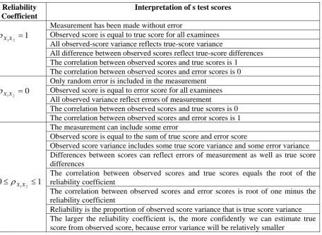
Yen and Allen (1979, p.76), offer a summary of applying the reliability coefficient in interpreting test scores. The summary is quoted in table 2.3.2.1.

Reliability Coefficient

Interpretation of s test scores

Measurement has been made without error

Observed score is equal to true score for all examinees All observed-score variance reflects true-score variance 1

2 1X =

X

ρ

All difference between observed scores reflect true-score differences The correlation between observed scores and true scores is 1

The correlation between observed scores and error scores is 0 Only random error is included in the measurement

Observed score is equal to error score for all examinees All observed variance reflect errors of measurement 0

2 1X =

X

ρ

The correlation between observed scores and true scores is 0 The correlation between observed scores and error scores is 1 The measurement can include some error

Observed score is equal to the sum of true score and error score

Observed score variance includes some true score variance and some error variance Differences between scores can reflect errors of measurement as well as true score differences

The correlation between observed scores and true scores equals the root of the reliability coefficient

The correlation between observed scores and error scores is root of one minus the reliability coefficient

1 0

2

1 ≤

≤

ρ

XX

Reliability is the proportion of observed score variance that is true score variance The larger the reliability coefficient is, the more confidently we can estimate true score from observed score, because error variance will be relatively smaller

2.4.0 Two popular Formulae for Estimating Reliability

In this section, two popular formulae for estimating test score reliability are briefly described.

Coefficient alpha is used when parallel test forms are not available, where as the Spearman- Brown Formula is used when parallel test forms are available.

2.4.1 Internal-Consistency Reliability

Internal-consistency reliability is estimated using one test administration. A test is divided into two or more subtests, say, N subtests. The variances of scores of the subtests and the variance of the total test score are used to estimate the reliability of the test by using the formula (Yen & Allen1979, pp. 83-84) stated below:

⎥

⎥

⎥

⎥

⎦

⎤

⎢

⎢

⎢

⎢

⎣

⎡

−

⎥⎦

⎤

⎢⎣

⎡

−

=

≥

∑

= 2 1 2 2

1

2 1 X N i Y X X X i

N

N

σ

σ

σ

α

ρ

, (2.4.1.1)

where X is the observed score for a test formed from combining N subtests, , is the population variance of X, is the population variance of the i

∑

= = N i i Y X 1 2 X

σ

2 i Y

σ

th

subtest, , and N is the number of subtests which combine to form X.

i

Y

Equation 2.4.1.1 shows that coefficient Alpha is the lower bound of the test reliability, meaning that low Alpha does not provide good information about the actual reliability of a test.

Corollary:

1. If each subtest,

Y

i, is a dichotomous item, equation 2.5.1.1 takes the following special form:

(a)

⎥

⎥

⎥

⎥

⎦

⎤

⎢

⎢

⎢

⎢

⎣

⎡

−

−

⎥⎦

⎤

⎢⎣

⎡

−

=

≥

∑

= 2 1 2

)

1

(

1

20

2 1 X N i i i X X X

p

p

N

N

KR

σ

σ

ρ

, (2.4.1.2)

where

p

_i is the proportion of examinees getting item i correct.

⎥

⎦

⎤

⎢

⎣

⎡

−

−

⎥⎦

⎤

⎢⎣

⎡

−

=

≥

2 2

)

1

(

1

21

2 1 X X X X

p

p

N

N

N

KR

σ

σ

ρ

(b) (2.4.1.3)

p

is the average of the p-values. where

2.4.2 The Spearman-Brown Formula

2 1X

X

ρ

The Spearman-Brown formula expresses the reliability, , of a test in terms of the reliability,

1

YY

1 1 2 1

)

1

(

1

_YY YY X X

N

N

ρ

ρ

ρ

−

+

=

, (2.4.2.1)

where X=the observed score for a test formed from combining N subtests, , is a subtest score that is a part of X,

∑

= = N i i Y X 1 i

Y

2 1X X

ρ

2 1Y Y

ρ

is the population reliability of X, is the population reliability of any

Y

_i, N is the number of parallel test scores that are combined to form X.

2.5.0 Standard Errors of Measurement and Confidence Intervals

When the discrepancy between an examinee’s true score and observed score from a test is interpreted, confidence intervals are commonly used to show the interval in which the expected score is likely to fall. Standard error of measurement is used to calculate the confidence interval. The formula for the estimated standard error of measurement is

2 1

1

_{X X}

X

E

σ

ρ

σ

=

−

, (2.5.0.1)

X

σ

is the standard deviation for the observed scores for the entire examinee group and where

2 1X

X

ρ

is the test reliability estimate.

The confidence interval for an examinee’s true score can be constructed as E

c E

c

T

x

z

z

x

−

σ

≤

≤

+

σ

, (2.5.0.2)

E

σ

where x is the observed score for the examinee, is estimated standard error of measurement, and is the critical value of the standard normal deviate at the desired probability level.

c

z

Item Analysis for Booklet 11

Number of observations = 50 Number of items = 30 Results based on raw (unweighted) scores Mean = 22.480 S.D. = 4.535 Alpha = .788

The case information contains test reliability coefficient alpha estimated for a test consisting of 30 dichotomous items administered to 50 examinees. Alpha is 0.788 and standard deviation is 4.535. The observed scores of the examinees on this test consist of true scores and random errors.

The magnitude of the random errors inherent in the test is 2.089. The mean of the true scores of the examinees may fall between 18.30 and 26.66 at 96 % confidence interval.

On the whole, this test is a good test. The mean of the observed scores of the examinees is close to the mean of their true scores.

Item Analysis for Booklet 12

Number of observations = 45 Number of items = 30 Results based on raw (unweighted) scores Mean = 23.822 S.D. = 3.702 Alpha = .711

The case information contains test reliability coefficient alpha estimated for a test consisting of 30 dichotomous items administered to 45 examinees. Alpha is 0.711 and standard deviation is 3.702. The observed scores of the examinees on this test consist of true scores and random errors.

The magnitude of the random errors inherent in the test is 2.00. The mean of the true scores of the examinees may fall between 19.82 and 27.82 at 96 % confidence interval.

On the whole, this test is a good test. The mean of the observed scores of the examinees is close to the mean of their true scores.

A case from the Project

2.6.0 Validity

Test scores are used for different purposes. For example, test scores are used for making placement decision, diagnosing learning difficulties, awarding grades, making admission decision, writing instructional guidance, setting future criterion, licensing and many more. In these examples, test scores provide scientific rationale for making inferences about examinees’ behaviors in relation to their test scores. The test makers and the test users apply validity studies to make the inferences derived from the test scores useful for making decisions.

Glas et al., (2003, p.100) describe validity as the meaning, usefulness and correctness of the conclusions made from the test scores. Glas et al., ( 2003, p.100, cf. Messick, 1989, 1995) define validity as “an overall evaluative judgment of the degree to which empirical evidence and theoretical rationales support the adequacy and appropriateness of interpretations and actions based on test scores or other modes of assessment”. Algina & Crocker (1986, p.217, cf. Cronbach, 1971) offer a procedural aspect of validity by emphasizing “validation as the process by which a test developer or test user gathers evidence to support the kinds of inferences that are to be drawn from test scores”.

Lord and Novick (1968, p.61) define validity coefficient of measurement X with respect to a second measurement Y as the absolute value of the correlation coefficient

Y X

XY

XY

σ

σ

σ

ρ

=

. (2.6.0.1)

Implicit in the definitions of validity is the need to identify and describe the desired inferences that are to be drawn form the test scores before conducting the validation studies. The major types of validity are content validity, criterion validity and construct validity.

2.6.1 Content Validity

• Defining the performance domain of interest

• Selecting a panel of qualified experts in the content domain

• Providing a structured framework for the process of matching items to the performance domain

• Collecting and summarizing the data from the matching process

The proposed steps may be accompanied by a check list of questions presented in table 2.6.1.1 to assist preliminary planning tasks for the content validation study.

Q.No. Question Yes No

1 Should domain objectives be weighted to reflect their importance? 2 How the item- domain objective mapping task should be structured? 3 What aspects of the item should be examined?

4 How should content validation study result be summarized? Table 2.6.1.1: Check list of questions for planning a content validation study

2.6.2 Criterion Validity

Glas et al., (2003,p.101) define criterion validity as the extent to which the test scores are empirically related to criterion measures. Criterion-related validity exists in two forms known as (1) predictive validity and (2) concurrent validity. Predictive validity involves using test scores to predict criterion measurement that will be made at some point in the future, where as concurrent validity is the correlation between test scores and criterion measurement when both are obtained at the same time. Criterion-related validation study is used when a test user wants to make an inference from the examinee’s test score to performance on some real behavioral variable of practical importance.

Algina & Crocker (1986, p.224) have proposed the following steps for criterion related validation study:

• Identify a suitable criterion behavior and a method for measuring it.

• Identify an appropriate sample of examinees representative of those for whom the test will automatically be used.

• Administer the test and keep a record of each examinee’s score.

• When the criterion data are available, obtain a measure of performance on the criterion for each examinee.

• Determine the strength of the relationship between test scores and criterion performance.

Regression analysis can be applied to establish criterion validity. An independent variable could be used as a predictor variable, X (Exam scores), and dependent variable, the criterion variable, Y (Grade point averages). The correlation coefficient between X and Y is called validity coefficient. It can be shown that the prediction of Y for the ith person is

(

X

X

)

Y

S

S

r

Y

_i

X Y XY

i

⎟⎟

−

+

⎠

⎞

⎜⎜

⎝

⎛

=

ˆ

_{, (2.6.2.1)}

where

Y

ˆ

_iis the future grade point average,

Y

is the mean of the grade point averages, is the correlation coefficient of exam score X and grade point average Y, is the standard deviation of the grade point averages, is the standard deviation of the exam scores, is the exam score of i

XY

r

Y

S

X

S

X

_i th

examinee.

This result can be expressed in confidence intervals by using the formula , where is the critical value from the normal table.

X Y c

i

z

s

2.6.3 Reliability of Predictor and Criterion Validity

When reliability coefficient is expressed as 2

2

1X XT

X

ρ

ρ

=

, (2.6.3.1)

it is clear that a test score cannot correlate more highly with any other variable than it can with its own true score. The maximum correlation between an observed test score and any other variable is

XT X

X

ρ

ρ

′

=

. (2.6.3.2)

XY

ρ

ρ

XY

If test, X, is used to predict a criterion, Y, then is the validity coefficient. As cannot not be larger than

ρ

XT ,

ρ

XY cannot be larger than

ρ

_XX′ , meaning that the square root of the reliability is the upper bound of the validity coefficient,

ρ

_XY

≤

ρ

_XX′ . Therefore, the reliability of the test affects the validity of the test.

XY

ρ

If both a test score, X, and criterion score, Y, are unreliable, the validity coefficient, , may be attenuated relative to the value of the validity coefficient that would be obtained if X and Y did not contain measurement error. Yen & Allen (1979, p.98, cf. Spearman, 1904) present the correction for attenuation as below:

Y Y X X

XY T

T_{X Y}

′ ′ =

ρ

ρ

ρ

ρ

, (2.6.3.3)

XY

ρ

Y XT T

ρ

is the correlation between the true score for X and the true score for Y,

where is the

correlation of observed scores X and Y containing error of measurement,

ρ

_XX′is the reliability of observed score X,

ρ

_YY′is the reliability of observed score Y.

Equation 2.6.3.3 expresses the correlation between true scores in terms of the correlation between observed scores and the reliability of each measurement. Lord and Novick (1968, p.70) interpret equation 2.7.3.3 as “giving the correlation between the psychological constructs being studied in terms of the observed correlation of the measure of these constructs and the reliabilities of these measures”.

2.6.4 Construct Validity

Construct validity is the degree to which a test measures the theoretical construct or trait that it was designed to measure (Lord & Novick, 1968, p.278). Construct validation study is usually conducted by analyzing the observed score correlations of a test with another test based on the theory underlying the constructs being measured. If the theory of the constructs predict the two tests to correlate, then there should be appreciable correlation between the two tests for the tests to be valid, otherwise the tests do not measure the constructs. Yen & Allen (1979,pp.108-109) propose (1) group differences, (2) changes due to experimental interventions, (3) correlation and (4) process as the possible predictions which can be made during construct validation study, besides content and criterion validities.

Algina & Crocker (1986, p.230) have summarized the following steps as the general steps involved in conducting a construct validation study:

hypotheses should be based on an explicitly stated theory that underlies the construct and provide its syntactic definition.

• Select (or develop) a measurement instrument which consists of items representing behaviors that are specific, and concrete manifestations of the construct.

• Gather empirical data which will permit the hypothesized relationships to be tested.

• Determine if the data are consistent with the hypotheses and consider the extent to which the observed findings could be explained by rival theories or alternative explanations (and eliminate these if possible).

2.7.0 Summary

CTT describes the relationship among observed score, true score and error of measurement. An observed score is the sum of true score and error of measurement. Expected value of the observed scores is the true score. Error score and true scores on a single test are uncorrelated. Error scores on two different tests are uncorrelated. Error scores on one test are uncorrelated with the true scores on another test. Two tests are parallel only when their corresponding true scores and error scores are equal. Essentially

τ

equivalent tests have same true scores and different additive constant.

Test reliability is the squared correlation between observed score and true score of the test. Two types of errors of measurement are systematic error of measurement and random error of measurement. For two parallel tests, the reliability coefficient is the correlation of the observed scores of one test with the observed scores of the other test. Reliability coefficient is the ratio of true score variance to observed score variance of a test. Reliability is the square of the correlation between observed score and true score. Reliability is the ratio of one minus the ratio of error score variance to observed score variance. Reliability is commonly estimated by using internal consistency reliability formula and Spearman-Brown Formula. Confidence interval is used to report true scores.

Validity is the absolute value of the correlation coefficient of two measurements. Three types of validity are content validity, criterion validity and construct validity. Criterion validity can be obtained by using regression analysis. Square root of the reliability is the upper bound of the validity.

2.8.0 References

Algina, J. & Crocker, L. (1986). Introduction to Classical and Modern Test Theory, Holt, Rinehart and Winston.

Glas, C.A.W. et al.(2003). Educational Evaluation, Assesment, and Monitoring, A Systemic Approach, Sweets & Zeitlinger Publishers

Lord, M. F. & Novick, R.M.(1968). Statistical Theories of Mental Test Scores, Addison-Wesley Publishing Company.

Chapter 3

Item Parameters in CTT Context

3.0.0 Introduction

Item bank will be functional when it has large reserve of good items. The quality of the items in an item bank is judged based on their parameters like item difficulty, item discrimination, item reliability and item validity statistics. These item parameters help test makers to choose the right items in accordance with the construct of interest when making a test.

In this chapter the item parameters are discussed in the context of CTT.

3.1.0 Item Difficulty

Item difficulty (sometime known as item facility) is the proportion of examinees who answer an item correctly (Algina & Crocker 1986, p.90). Item difficulty in the context of CTT is sample dependent. Its values will remain invariant only for groups of examinees with similar levels. Item difficulty is often referred to as p-value in CTT. This value represents the percentage of a certain group of examinees who selected a particular response. A p-value can be calculated for each response, the correct answer and each of the distractors, by dividing the number of individuals that selected a particular response by the total number of individuals in the group of interest. Mathematically, the definition based expression for p-value is

N pij

j item on i score with persons of

Number

= , (3.1.0.1)

where is the p-value for item j with score i and N is the total number of examinees who attempted the item j.

ij

p

Corollary:

(1) For dichotomous items, p_j is equal to mean score of item j. (2) For polytomous items,

)

(

max

)

)(

(

ij all

ij ij j

X

X

p

p

i

=

, where (Xij)is the is score i on item j. (3.1.0.2)

X

(3) The mean of test score ( ) is

∑

=

=

N j

j

p

X

1

, (3.1.0.3)

where N is number of items in the test.

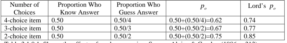
Depending on the number of choices involved in dichotomous items, the p-values of items at which the maximum true score variance would be obtained also differ due to random guessing by those examinees who do not know the correct answer. Algina & Crocker (1986, p.313) provide an expression for the p-value of an item at which the true score variance would be maximum as

m

p_o =0.50+0.50, (3.1.0.4)

Number of Choices

Proportion Who Know Answer

Proportion Who

Guess Answer o

p

Lord’s

p

o

4-choice item 0.50 0.50/4 0.50+(0.50/4)=0.62 0.74 3-choice item 0.50 0.50/3 0.50+(0.50/2)=0.67 0.77 2-choice item 0.50 0.50/2 0.50+(0.50/2)=0.75 0.85 Table 3.1.0.1: Shows the effects of random guessing. Source: Algina & Crocker (1986, p.313).

From table 3.1.0.1, it is clear that an item difficulty increases with increase in number of alternatives when multiple-choice item format is used in the test. Lord’s is the demonstration made by Lord (Algina & Crocker, 1986, p. 313) which suggests that a test reliability can be improved by choosing items with p-values even higher than those computed by adjusting for random guessing.

o

p

3.1.1 Role of Item P-values in Item Analysis

The p-values of items will be different for different items of a test depending on the types of examinees. If the items are difficult, then their values will be low. If the items are easy, then p-values will be high.

The p-value of an item can provide general guidance when analyzing an item. If the p-value is very low (in the range of 0.00 to 0.20), then the item is very hard and the possibility that the item has been miskeyed or that there is more than one correct answer to the question should be examined. Very low p-value is also indicative of floor effect.

If the p-value is greater than 0.95, then the correct answer is probably too obvious for the test population. The very high p-value is also indicative of ceiling effect. The items with p-values less than or equal to 0.20 and greater than or equal to 0.95 should be deleted or revised to present a greater challenge to the test candidates. If the p-value is zero for any response, this is called a "Null distractor." Null distractors are indicative of obvious answers, nonparallel distractors, or nonsensical distractors.

3.2.0 Item Variance

Item variance is the square of the item standard deviation. Mathematically, item-variance can be expressed as

(

)

N

X

_{ij j} j

∑

−

=

2

2

μ

σ

, (3.2.0.1)

where Xij= Score of examinee i on item j,

μ

j= mean score on item j, and N= number of examinees. Corollary:

For dichotomous items

(1) item variance can be calculated by using p-values as j

j

j

=

p

q

2

σ

, (3.2.0.2)

where q_j =1-p_j.

(2) standard deviation of the item can be calculated as j

j

j = p q

σ

. (3.2.0.3)

Item variance indicates the variability of the answers to the item. A low item variance indicates that most students selected or presented the same response to the item (not necessarily the correct one). A high item variance means that a near even number of students selected or presented a particular response.

3.3.0 Item Discrimination

Examinees differ in their abilities. It is conventional to expect high scores, average scores and low scores and other scores which incline to fall in any of these groups. Therefore, while analyzing test items, one of the objects is to select items which have potential to separate examinees into different categories of performance based on their abilities. This means that a test item should have characteristics capable of being scored correctly by high ability examinees and incorrectly by low ability examinees. The items which have such properties are discriminative. These items discriminate examinees who know answers from examinees who do not know answers.

In the following section, three commonly used item discrimination statistics are described.

3.3.1 Index of Item Discrimination

Index of item discrimination is applicable only to dichotomously scored items. To calculate item discrimination index, examinees are separated into two groups based on their total test scores with respect to the cut scores. The two groups are categorized as upper group and lower group . The index of discrimination (D) is calculated as

)

(

p

u

(

p

l

)

l

u

p

p

D

=

−

. (3.3.1.1)

3.3.1.1 Role of Index of Discrimination in Item Analysis

Algina & Crocker (1986, p.315,cf. Ebel, 1965) provide the following guidelines for interpretation of D-values when the groups are established with total test score as the criterion:

If D

≥

0

.

40

, the item is functioning quite satisfactorily. If

0

.

30

≤

D

≤

0

.

39

, little or no revision is required.

If

0

.

20

≤

D

≤

0

.

29

, the item is marginal and needs revision. If

D

≤

0

.

19

, the item should be eliminated or completely revised.

3.3.2 Point Biserial Correlation

The point biserial correlation reflects the item-test correlation when a discrete binary variable (correct vs incorrect response to the item) is correlated with a continuous variable (total test score). Algina & Crocker (1986, p.317) state the mathematical sentence for point biserial correlation as

q p

X X

pbis ×

− = +

σ

μ

μ

ρ

( ) , (3.3.2.1)

+

μ

is the mean criterion score for those who answer the item correctly,

μ

_X

where is the mean criterion