Study on real-time correction of site amplification factor

(1)

https://doi.org/10.5194/nhess-19-2827-2019 © Author(s) 2019. This work is distributed under the Creative Commons Attribution 4.0 License.

Study on real-time correction of site amplification factor

Quancai Xie1, Qiang Ma1, Jingfa Zhang2, and Haiying Yu1

1_{Key Laboratory of Earthquake Engineering and Engineering Vibration, Institute of Engineering Mechanics, China} Earthquake Administration, Harbin, 150080, China

2_{Key Laboratory of Crustal Dynamics, Institute of Crustal Dynamics, China Earthquake Administration,} Beijing, 100085, China

Correspondence:Quancai Xie ([email protected])

Received: 24 December 2018 – Discussion started: 4 February 2019

Revised: 6 October 2019 – Accepted: 28 October 2019 – Published: 13 December 2019

Abstract. The site amplification factor was usually consid-ered to be scalar values, such as amplification of peak ground acceleration or peak ground velocity, or increments of seis-mic intensity in the earthquake early warning (EEW) system or seismic-intensity repaid report system. This paper focuses on evaluating an infinite impulse recursive filter method that could produce frequency-dependent site amplification and compare the performance of the scalar-value method with the infinite impulse recursive filter method. A large num-ber of strong motion data of IBRH10 and IBRH19 of the Kiban Kyoshin network (KiK-net) triggered in more than 1000 earthquakes from 2004 to 2012 were selected care-fully and used to obtain the relative site amplification ra-tio; we model the relative site amplification factor with a ca-sual filter. Then we make a simulation from the borehole to the surface and also simulate from the front-detection sta-tion to the far-field stasta-tion. Compared to different simulasta-tion cases, it can easily be found that this method could produce different amplification factors for different earthquakes and could reflect the frequency-dependent nature of site amplifi-cation. Through these simulations between two stations, we can find that the frequency-dependent correction for site am-plification shows better performance than the amam-plification factor relative to velocity (ARV) method and station correc-tion method. It also shows better performance than the aver-age level and the highest level of the Japan Meteorological Agency (JMA) earthquake early warning system in ground motion prediction. Some cases in which simulation did not work very well were also found; possible reasons and prob-lems were analyzed and addressed. This method pays atten-tion to the amplitude and ignores the phase characteristics; this problem may be improved by the seismic-interferometry

method. Frequency-dependent correction for site amplifica-tion in the time domain highly improves the accuracy of pre-dicting ground motion in real time.

1 Introduction

In recent decades, real-time strong ground motion predic-tion has become an important part of earthquake early warn-ing (EEW) systems. In the world, there are many countries and regions that deploy operational earthquake early warning systems, like Mexico (Espinosa-Aranda et al., 1995, 2009), Japan (Kamigaichi, 2004; Hoshiba et al., 2008; Nakamura et al., 2009), Taiwan (Wu and Teng, 2002; Hsiao et al., 2009), Turkey (Erdik et al., 2003; Alcik et al., 2009), and Roma-nia (Wenzel et al., 1999; Ionescu et al., 2007). Also there are some earthquake early warning systems under development and testing, like in the Unites States (Allen and Kanamori, 2003; Allen et al., 2009; Bose et al., 2009), Italy (Zollo et al., 2006, 2009), and China (Peng et al., 2011).

(2)

2828 Q. Xie et al.: Study on real-time correction of site amplification factor

and the high-sensitivity seismograph network (Hi-net) were used to determine the hypocenter of the Japan Meteorologi-cal Agency earthquake early warning system. In order to dis-seminate the warning quickly, hypocenter estimation should be done just after the first detection of the P phase at a sin-gle station. In order to ensure the reliability of the estima-tion, the B-delta method (Odaka et al., 2003) and network method (Horiuchi et al., 2005; Horiuchi et al., 2009) are used in combination. Usually, the current Japan Meteorological Agency earthquake early warning system works well. But after the main shock of the 2011 great T¯ohoku earthquake, the earthquake early warning system did not work well due to high aftershock activity and high background noise as well as power failure and wiring disconnection (Hoshiba et al., 2011). Earthquakes that occurred simultaneously in dif-ferent locations nearby also caused the system to provide false information. The site amplification factor was usually considered to be scalar values, such as the amplification of peak ground acceleration or peak ground velocity and incre-ments of seismic intensity, in the conventional earthquake early warning system. There are some research papers on improving the site amplification factor for more accuracy in calculating Japan Meteorological Agency seismic intensity in the Japanese earthquake early warning system (Iwakiri et al., 2011). Among them, we choose the new idea proposed by Hoshiba (2013) and use it to design a casual filter for modeling the site amplification factor of Kiban Kyoshin net-work (KiK-net) stations. We focus on a full evaluation of the performance of this method by selecting a large number of KiK-net data triggered in more than 1000 earthquakes; then we a make simulation from the borehole to the sur-face and also simulate from the front-detection station to the far-field station. Then we compare the statistical simulation results with other methods considering the accuracy of the seismic-intensity prediction and clarify the advantages and some problems that need to be considered when utilizing it in earthquake early warning systems.

2 Data

The hypocenter parameters, including the origin time, loca-tion of hypocenter, and magnitude, were obtained from the JMA seismic catalogue. The strong motion data were down-loaded from the following website: http://www.kyoshin. bosai.go.jp/ (last access: 23 September 2019). The advan-tage of this network is that all stations have a borehole of 100 m or more in depth, with accelerographs installed both on the ground surface and at the bottom of boreholes. The site information measured in the boreholes includes soil type along with P- and S-wave velocity profiles. The sampling frequency is 200 Hz for the records before November 2007 and is 100 Hz thereafter. In this analysis, we use records observed at two stations. One of them, with the site code IBRH10, has been in operation since 1 September 2000, and

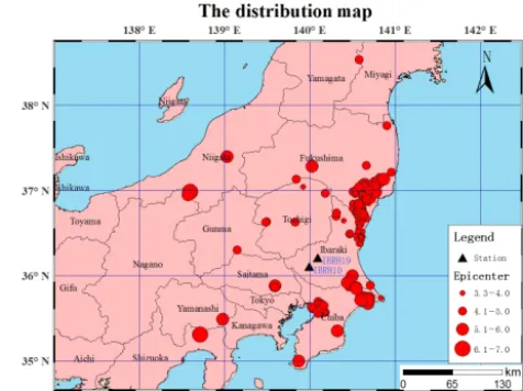
Figure 1.The station and epicenter distribution map used for this research.

the other station, with site code IBRH19, has been in opera-tion since 15 May 2004. Until 31 December 2012, IBRH10 and IBRH19 recorded 1119 and 910 events, respectively. We selected 673 strong ground motion records which were recorded at the surface and by the borehole sensor when both of these stations were triggered by an earthquake. The in-ner distance between IBRH10 and IBRH19 is 14.6 km. We selected strong motion data with a hypocenter distance at least 3 times larger than the inner distance. The number of earthquakes is up to 553, and the range of magnitude was be-tween 3.3 and 9. The recording time spans from 16 May 2004 to 31 December 2012. Excluding the earthquake which oc-curred in the sea area, the number of earthquakes with mag-nitudes ranging from 3.3 to 7 adds up to 208 (Fig. 1); 20 m of soft sediment exists at the station IBRH10. The layer of rock appears at the depth of 518 m. The IBRH19 is almost a completely rock site station. The site profiles can be down-loaded from the KiK-net website (http://www.kyoshin.bosai. go.jp/kyoshin/db/index_en.html?all, last access: 23 Septem-ber 2019).

3 Theory and methodology

(3)

ampli-Figure 2.Comparison of the method proposed by Hoshiba with the network method (modified after Hoshiba, 2013).

fication factor can be reproduced by a casual recursive fil-ter based on the historical relative spectral ratio between two stations. In this method the far-field simulated waveform can be obtained by real-time filtering of the observed waveform recorded in the front detection station.

Seismic ground motion is often modeled by convolution of the source, propagation, and site amplification factors. Site amplification factors play an important role in determining seismic wave amplitude other than the propagation effect and source effect. Usually, the site amplification factor was evalu-ated in the frequency domain. However, for earthquake early warning systems, it is not suitable, as this procedure needs some length of windowed waveform for fast Fourier trans-form (FFT) in the frequency domain. In many previous stud-ies, site amplification factors are estimated using the follow-ing equation (Iwata and Irikura, 1988):

Okl(f )=Sk(f )Gl(f )Tkl(f ), (1)

wheref is frequency in hertz; Okl(f ),Sk(f ),Gl(f ), and

Tkl(f )represent the observed seismic spectrum from eventk

at sitel, the source spectrum characterizing the eventk, the site amplification factor at sitel, and the propagation factor between event k and site l, respectively; andf is the fre-quency of the seismic waves.

The frequency-dependent relative site amplification fac-tors are assumed to be modeled by the following linear sys-tem of first-order and second-order filters:

F (s)=G0 YN

n=1 _ω

2n

ω1n

·s+ω1n s+ω2n

YM

m=1( ω2m

ω1m

)2

·s 2₊₂_h

1mω1m+ω21m

s2₊₂_h

1mω1m+ω2₂_m

, (2)

whereN andMstand for the numbers of the first-order and second-order filters, respectively, ands=iω. Hereωvalues are angular frequencies, and h values are damping factors that characterize the frequency dependence.s2+2hω+ω_m2

represents a damping oscillation (Hoshiba, 2013). G0,ω1n,

ω2n,ω1m, andω2mare estimated for given values ofNandM

by using the least-squares method on logarithmic scales. We focus on the amplitude characteristics, ignoring phase char-acteristics. The bilinear transform (also known as Tustin’s method) is introduced as

s= 2 1T

1−Z−1

1+Z−1, (3)

which is used in digital signal processing and the discrete-time control theory to transform continuous-discrete-time system rep-resentations into discrete time. Then the pre-warping equa-tion,

ω→ 2

1T tan( ω1T

2 ), (4)

is applied toω1n,ω2n,ω1m, andω2m. Next the transfer

func-tionF (z)is obtained, where1T is the sampling interval of the digital waveforms andz=exp(s1T ). Equation (3) and (4) are the necessary procedures for obtaining the coefficients of a causal recursive filter for real-time processing.

4 Result analysis 4.1 Spectral ratios

(4)

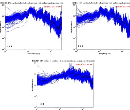
Figure 3.Surface-to-borehole spectral ratios at IBRH10:(a)EW2/EW1,(b)NS2/NS1, and(c)UD2/UD1. The blue lines stand for the spectra ratio for every earthquake event, and the black line stands for the average spectra ratio for all the events.

4.2 Simulation from borehole to surface

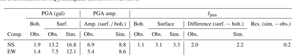
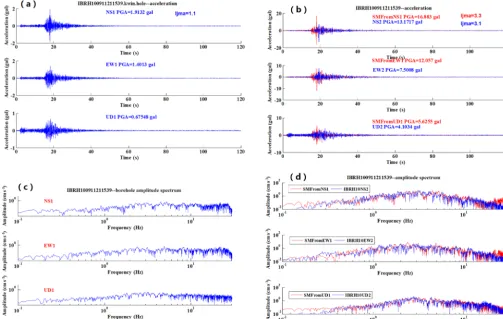
Firstly, we make the simulation from the borehole to the sur-face, although it is not useful for the earthquake early warn-ing system. However, it could be used to make a full evalua-tion of this method. We use the strong moevalua-tion data recorded by the IBR10 borehole sensor to simulate the surface sta-tion accelerasta-tion waveforms and spectrum. Figure 6a to d show the simulation results for the M4.5 earthquake which occurred on 21 November 2009. The information about the site amplification factors and the increment of seismic inten-sity are summarized in Table 1. In the table, amp., obs., sim., comp., res., surf., and boh. are the abbreviations of amplifica-tion, observaamplifica-tion, simulaamplifica-tion, component, residual, surface, and borehole respectively.

Figure 7a to d show the simulation results for the M4.6 earthquake which occurred on 7 December 2012. The infor-mation about the site amplification factors and the increment of seismic intensity are summarized in Table 2.

For these two examples, comparing the simulated acceler-ation and spectrum with the observed acceleracceler-ation and spec-trum of the surface records, the results were simulated well. The different amplifications of maximum acceleration be-tween Tables 1 and 2 reflect the differences of the frequency contents of the incident waveforms that cannot be reproduced by a scalar site amplification factor (e.g., amplification of peak ground acceleration or peak ground velocity or incre-ment of seismic intensity).

(5)

Figure 4.Surface-to-borehole spectral ratios at IBRH19:(a)EW2/EW1,(b)NS2/NS1, and(c)UD2/UD1. The blue lines stand for the spectra ratio for every earthquake event, and the black line stands for the average spectra ratio for all the events.

Table 1.Information forM4.5earthquake (IBRH100911211539).

PGA (gal) PGA amp. Ijma

Boh. Surf. Amp. (surf./boh.) Boh. Surface Difference (surf.−boh.) Res. (sim.−obs.)

Comp. Obs. Obs. Sim. Obs. Sim. Obs. Obs. Sim. Obs. Sim.

NS 1.9 13.2 16.8 6.9 8.8 1.1 3.1 3.3 2.0 2.2 0.2

EW 1.4 7.5 12.1 5.4 8.6

UD 0.7 4.1 5.6 5.9 8.3

4.3 Simulation between front-detection station and far-field station

Then, using the surface strong motion data of IBRH19, we get simulated waveforms for IBRH10. Figure 9a–d show the simulation results for theM5.2earthquake which occurred on 19 February 2012. The information about site amplification factors and the increment of seismic intensity is summarized in Table 3.

(6)

accel-2832 Q. Xie et al.: Study on real-time correction of site amplification factor

Figure 5.Spectral ratios of IBRH10 to IBRH19 for(a)EW1,(b)EW2,(c)NS1, and(d)NS2. The blue lines stand for the spectra ratio for every earthquake event, and the black line stands the average spectra ratio for all the events.(e)UD1.(f)UD2. The blue lines stand for the spectra ratio for every earthquake event, and the black line stands for the average spectra ratio for all the events.

Table 2.Information forM4.6earthquake (IBRH101212070532).

Boh. Surf. Amp. (surf./boh.) Boh. Surf. Difference (surf.−boh.) Res. (sim.−obs.)

Comp. Obs. Obs. Sim. Obs. Sim. Obs. Obs. Sim. Obs. Sim.

NS 0.7 2.7 3.6 3.9 5.1 0.0 1.2 1.3 1.2 1.3 0.1

EW 0.6 3.3 4.0 5.5 6.7

(7)

Figure 6.An example of the results of simulation for IBRH100911211539:(a)the observed acceleration at the borehole,(b)the observed surface acceleration waveform (blue) compared with the simulated one (red),(c)the spectra of the observed borehole record, and(d)the spectra of the observed surface record (blue) compared with the simulated one (red).

Table 3.Information forM5.2earthquake (IBRH10 and IBRH19 for 201202191454).

IBRH19 IBRH10 Amp. (IBRH100/IBRH19) IBRH19 IBRH10 Res. (obs.−sim.)

Comp. Obs. Obs. Sim. Obs. Sim. Obs. Obs. Sim.

NS 17.7 50.9 69.7 2.8 3.9 2.2 3.5 3.7 0.2

EW 13.6 45.7 53.2 3.3 3.9

UD 11.2 23.7 38.9 2.1 3.5

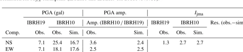
eration amplification factors for theM5.1earthquake which occurred on 14 April 2011 are 2.4, 2.5, and 3.9. Comparing the simulation results for these two earthquakes, the different amplification of acceleration between Tables 3 and 4 shows the different frequent content of the waveforms that cannot be reproduced by a scalar site amplification method.

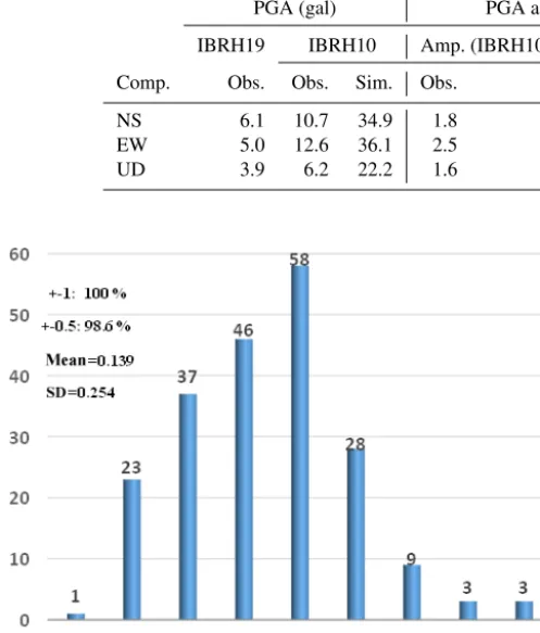
Although most of the simulation results show good perfor-mance, cases exist in which the simulation did not work well. For example, Fig. 11a–d show the simulation results for the

M5.3earthquake that occurred on 16 March 2011. The infor-mation about the site amplification factors and the increment of seismic intensity is summarized in Table 5. Comparing the

(8)

Figure 7.An example of the results of simulation for IBRH101212070532:(a)the observed acceleration at the borehole,(b)the observed surface acceleration waveform (blue) compared with the simulated one (red),(c)the spectra of the observed borehole record, and(d)the spectra of the observed surface record (blue) compared with the simulated one (red).

NS 7.1 25.4 16.7 3.6 2.4 1.3 2.7 2.7 0

EW 7.1 18.1 17.6 2.5 2.5

UD 4.3 14.6 16.7 3.4 3.9

velocity at the ground surface relative to the engineering bedrock of averaged S-wave velocity – 700 m s−1) based on topographic data. Iwakiri et al. (2011) proposed the station correction method. The station correction method is based on site amplifications obtained empirically from observed seismic-intensity data.

We compared the performance of this method with the ARV method and station correction method. For the ARV

(9)

NS 6.1 10.7 34.9 1.8 5.7 1.5 2.7 3.8 1.1

EW 5.0 12.6 36.1 2.5 7.2

UD 3.9 6.2 22.2 1.6 5.7

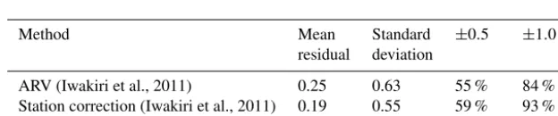
Figure 8. The seismic-intensity residuals between observed data and simulated data.

seismic-intensity error is 74.74 % for all 11 years of data. The best case is 93.7 % in 2017, and the worst case is 34.6 % in 2010. From the analysis mentioned above, we can conclude that this method could improve the accuracy of the seismic-intensity estimation. It highly improves the accuracy of pre-dicting ground motion in real time and could be used in the earthquake early warning system.

5 Discussion

Through comparing different simulation cases, one can easily see that the frequency-dependent correction of the site amplification factor could produce different amplifica-tion factors for different earthquakes. It could produce the frequency-dependent site amplification factor and highly im-proves situations in which scalar-value site amplification methods could not produce different amplification factors for different earthquakes. It skips the procedure to calculate the EEW magnitude and epicenter distance or hypocenter dis-tance using the starting portion of the waveform. We can ob-tain the waveform in real time at the target station. It highly improves the accuracy of predicting ground motion in real time compared with the scalar-value site amplification factor.

The simulation from the borehole to the surface is not suit-able for earthquake early warning systems, but it proves that this method shows good performance for simulating wave-forms of the target station in real time. For the purpose of earthquake early warning, we need to save a lot of lead time for warning the public, requiring the distance between two stations to be much larger. It means that the method has a relation to network density. We could use the frequency-dependent site implication factor to predict the seismic in-tensity more accurately in the seismic-inin-tensity quick report system and earthquake early warning system with high net-work density. For the purposes of earthquake early warn-ing, we need to use a large amount of historical ground mo-tion records to model the relative site amplificamo-tion and find the optional casual-filter parameter firstly. In the area with a sparse network and low seismicity, we could not get the relative site amplification easily because of a small number of strong motion records. We need to consider other meth-ods for estimating the relative site amplification factor. We can adopt a method such as the coda normalization method (Phillips and Aki, 1986) or generalized spectrum inversion method (Iwata and Irikura, 1986; Kato et al., 1992).

There are cases in which some simulations did not work very well; 1.9 % of the seismic-intensity residuals are larger than 1. One of possible reasons is the azimuth dependency of site amplification (Cultrera et al., 2003). We did not consider azimuth dependency in designing the frequency-dependent filter for the site amplification factor. If we design multiple frequency-dependent correction filters for the site amplifica-tion factor regarding the azimuth dependency of site amplifi-cation, we would be able to predict the target ground motion more precisely. Another possible reason is the accuracy of the input relative spectral ratio. This situation may be im-proved by more precisely characterizing the input spectral ratio and complicated filter design. For example, we can use a large number of first- and second-order filters to model the spectral ratio, but it is more complicated and time-consuming for the hardware design when the number of filters grows larger. We need to make a trade-off between the accuracy of the input spectral ratio and the difficulty of the filter design.

(10)

Figure 9.An example of simulation from IBRH19 (surface) to IBRH10 (surface) for the earthquake 201202191454:(a)the observed surface acceleration for IBRH19,(b)the observed surface acceleration waveform (blue) compared with the simulated one (red),(c)the spectral ratio of observed surface record for IBRH19, and(d)the observed spectra of surface record at IBRH10 (blue) compared with the simulated one (red).

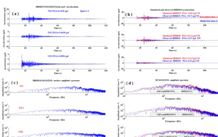
Table 6.The comparison results.

Method Mean Standard ±0.5 ±1.0

residual deviation

ARV (Iwakiri et al., 2011) 0.25 0.63 55 % 84 %

Station correction (Iwakiri et al., 2011) 0.19 0.55 59 % 93 %

This paper 0.35 0.36 69.7 % 98.1 %

system. This situation may be improved with the seismic-interferometry method (Yamada et al., 2010). Because the site amplification factor was assumed to be a linear system, the nonlinearity of weak ground motion and strong ground motion (Noguchi et al., 2012) was not taken into consider-ation in this study. More research is needed to solve these problems.

6 Conclusion

In this paper, we evaluate the infinite impulse recursive fil-ter method that models the relative site amplification fac-tor by hisfac-torical strong ground motion data and then imple-ments the relative site amplification factor with the casual filter. First, we calculated the spectrum ratio for IBRH10

and IBRH19; then we obtained the surface simulated ac-celeration time series and spectrum for IBRH10 from bore-hole records at IBRH10. Similarly, we obtained the IBRH10-simulated surface acceleration time series and spectrum from the surface strong ground motion records of IBRH19. Lastly, we calculated the seismic-intensity residual between the ob-served data and simulated data and then compared the ac-curacy with the previous method and statistical report. This method highly improves the accuracy of predicting ground motion in real time. The results show the following.

(11)

Figure 10.An example of simulation from IBRH19 (surface) to IBRH10 (surface) for the earthquake 201104140735:(a)the observed surface acceleration for IBRH19,(b)the observed surface acceleration waveform (blue) compared with the simulated one (red),(c)the spectral of observed surface record for IBRH19, and(d)the observed spectra of surface record at IBRH10 (blue) compared with the simulated one (red).

(12)

Figure 12. The seismic-intensity residuals between the observed data and simulated data.

Figure 13.The percent ratio diagram for 1◦seismic-intensity error in the current Japan EEW system.

standard deviation of these seismic-intensity residuals is 0.254; 98.6 % of these seismic-intensity residuals are less than 0.5, and 100 % of these seismic-intensity resid-uals are less than 1.

2. The spectra ratio is calculated between IBRH10 and IBRH19 surface records. Similarly, we use the infinite impulse recursive filter method to model the relative spectra ratio between two stations. The average seismic-intensity residual of these earthquakes is 0.35. The stan-dard deviation of these seismic-intensity residuals is 0.36; 69.7 % of these seismic-intensity residuals are less than 0.5, and 98.1 % of these seismic-intensity residuals are less than 1. This method shows better performance than the ARV method and station correction method. The average 1◦ seismic-intensity error of all 11 years of statistical data of the current Japan Meteorological Agency earthquake early warning system is 74.74 %. This method also shows better performance than the current operational Japan Meteorological Agency earth-quake early warning system. This method highly

im-proves the accuracy of predicting ground motion in real time.

Data availability. The hypocenter parameters, including the origin time, location of hypocenter, and magnitude, used in this study, which were routinely determined by JMA, were obtained from the JMA seismic catalog. The KiK-net strong motion data can be down-loaded from the NIED website (http://www.kyoshin.bosai.go.jp/, last access: 23 September 2019). We thank JMA and NIED for their hard work.

Author contributions. QX completed the core work and wrote the text content, QM and JZ were the technical directors in chief, and HY supervised the strong motion data processing and related analy-sis. All authors discussed the editor opinions and revised the paper.

Competing interests. The authors declare that they have no conflict of interest.

Acknowledgements. We thank Toshiaki Yokoi (BRI) and Mitsuyuki Hoshiba (MRI) for supervising Quancai Xie and providing useful suggestions for this study. We also thank Toshihide Kashima(BRI) for providing the program that we used for calculating the JMA seismic intensity.

Financial support. This work is partially supported by the Sci-entific Research Fund of the Institute of Engineering Mechan-ics, China Earthquake Administration (grant no. 2019B06), Na-tional Key Research and Development Program of China (grant no. 2018YFE0109800), National Natural Science Foundation of China (grant no. 41874059), and Seismological Science and Technology Spark Project (grant no. XH19071).

Review statement. This paper was edited by Filippos Vallianatos and reviewed by Hao Chen and three anonymous referees.

References

Alcik, H., Ozel, O., Apaydin, N., and Erdik, M.: A study on warning algorithms for Istanbul earthquake early warning system, Geophys. Res. Lett., 36, L00B05, https://doi.org/10.1029/2008GL036659, 2009.

Allen, R. M. and Kanamori, H.: The potential for earthquake early warning in southern California, Science, 300, 786–789, 2003. Allen, R. M., Brown, H., Hellweg, M., Khainovski, O., Lombard,

P., and Neuhauser, D.: Real-time earthquake detection and hazard assessment by ElarmS across California, Geophys. Res. Lett., 36, L00B08, https://doi.org/10.1029/2008GL036766, 2009. Bose, M., Hauksson, E., Solanki, K., Kanamori, H., and Heaton, T.

(13)

5.4 Chino Hills earthquake, Geophys. Res. Lett., 36, L00B03, https://doi.org/10.1029/2008GL036366, 2009.

Cultrera, G., Rovelli, A., Mele, G., Azzara, R., Caserta, A., and Marra, F.: Azimuth-dependent amplification of weak and strong ground motions within a faultzone (No-cera Umbra, central Italy), J. Geophys. Res., 108, 2156, https://doi.org/10.1029/2002JB001929, 2003.

Erdik, M., Fahjan, Y., Ozel, O., Alcik, H., Mert, A., and Gul, M.: Istanbul earthquake rapid response and the early warning system, B. Earthq. E., 1, 157–163, 2003.

Espinosa-Aranda, J. M., Jimenez, A., Ibarrola, G., Alcantar, F., Aguilar, A., Inostroza, M., and Maldonado, S.: Mexico City Seis-mic Alert System, Seismol. Res. Lett., 66, 42–52, 1995. Espinosa-Aranda, J. M., Cuellar, A., Garcia, A., Ibarrola, G., Islas,

R., Maldonado, S., and Rodriguez, F. H.: Evolution of the Mex-icanSeismic Alert System (SASMEX), Seismol. Res. Lett., 80, 694–706, 2009.

Horiuchi, S., Negishi, H., Abe, K., Kamimura, A., and Fujinawa, Y.: An automatic processing system for broadcasting earthquake alarms, B. Seismol. Soc. Am., 95, 708–718, 2005.

Horiuchi, S., Horiuchi, Y., Yamamoto, S., Nakajima, H., Wu, C., Rydelek, P. A., and Kachi, M.: Home seismometer for earthquake early warning, Geophys. Res. Lett., 36, L00B04, https://doi.org/10.1029/2008GL036572, 2009.

Hoshiba, M., Kamigaichi, O., Saito, M., Tsukada, S., and Hamada, N.: Earthquake early warning starts nationwide in Japan, EOS T. Am. Geophys. Un., 89, 73–80, 2008.

Hoshiba, M., Iwakiri, K., Hayashimoto, N., Shimoyama, T., Hirano, K., Yamada, Y., Ishigaki, Y., and Kikuta, H.: Outline of the 2011 off the Pacific coast of Tohoku Earthquake (Mw 9.0), Earth Plan-ets Space, 63, 547–551, 2011.

Hoshiba, M.: Real Time Correction of Frequency-Dependetnt Site Amplification Factors for Application to Earthquake Early Warn-ing, B. Seismol. Soc. Am., 103, 3179–3188, 2013.

Hsiao, N. C., Wu, Y. M., Shin, T. C., Zhao, L., and Teng, T. L.: Development of earthquake early warn-ing system in Taiwan, Geophys. Res. Lett., 36, L00B02, https://doi.org/10.1029/2008GL036596, 2009.

Ionescu, C., Bose, M., Wenzel, F., Marmureanu, A., Grigore, A., and Marmureanu, G.: Early warning system for deep Vrancea (Romania) earthquakes, in: Earthquake Early Warning Systems, edited by: Gasparini, P., 2007.

Iwata, T. and Irikura, K.: Separation of source, propagation and site effects from observed S-waves, Zisin II, 39, 579–593, 1986 (in Japanese with English abstract).

Iwata, T. and Irikura, K.: Source parameters of the 1983 earthquake sequence, J. Phys. Earth, 36, 155–184, 1988.

Iwakiri, K., Hoshiba, M., Nakamura, K., and Morikawa, N.: Im-provement in the accuracy of expected seismic intensities for earthquake early warning in Japan using empirically estimated site amplification factors, Earth Planets Space, 63, 57–69, 2011. Japan Meteorological Agency: The EEW statistical

re-port on the Japan Meteorological Agency EEW system [EB/0L], http://www.data.jma.go.jp/svd/eqev/data/study-panel/ eew-hyoka/10/shiryou1-1.pdf (last access: 20 November 2018), 2018 (in Japanese).

Kamigaichi, O.: JMA earthquake early warning, Journal of the Japan Association for Earthquake Engineering, 4, 134–137, 2004.

Kato, K., Takemura, M., Ikeura, T., Urao, K., and Uetake, T.: Pre-liminary analysis for evaluation of local site effects from strong motion spectra by an inversion method, J. Phys. Earth, 40, 175– 191, 1992.

Nakamura, H., Horiuchi, S., Wu, C., Yamamoto, S., and Ry-delek, P. A.: Evaluation of the real-time earthquake infor-mation system in Japan, Geophys. Res. Lett., 36, L00B01, https://doi.org/10.1029/2008GL036470, 2009.

Noguchi, S., Sato, H., and Sasatani, T: Characterization of nonlinear site response based on strong motion records at K-NET and KiK-net stations in the east of Japan., Proc. of 15th World Conference on Earthquake Engineering, Lisbon, Portugal, 24–28 September 2012, abstract number 3846, 2012.

Okada, T., Ashiya, K., Tsukuda, A., Sato, S., Ohtake, T., and Nozaka, D.: A new method of quickly estimating epicentral dis-tance and magnitude from a single seismic record, B. Seismol. Soc. Am., 93, 526–532, 2003.

Peng, H. S., Wu, Z. L., Wu, Y. M., Yu, S. M., Zhang, D. N., and Huang, W. H.: Developing a Prototype Earthquake Early Warn-ing System in the BeijWarn-ing Capital Region, Seismol. Res. Lett., 82, 394–403, https://doi.org/10.1785/gssrl.82.3.394, 2011. Phillips, W. S. and Aki, K.: Site amplification of coda waves from

local earthquakes in central California, B. Seismol. Soc. Am., 76, 627–648, 1986.

Wenzel, F., Onescu, M., Baur, M., and Fiedrich, F.: An early warn-ing system for Bucharest, Seismol. Res. Lett., 70, 161–169, 1999.

Wu, Y. M. and Teng, T. L.: A virtual subnetwork approach to earth-quake early warning, B. Seismol. Soc. Am., 92, 2008–2018, 2002.

Yamada, M., Mori, J., and Ohmi, S.: Temporal changes of subsurface velocities during strong shaking as seen from seismic interferometry, J. Geophys. Res., 115, B03302, https://doi.org/10.1029/2009JB006567, 2010.

Yamazaki, F., Noda, S., and Meguro, K..: Developments of early earthquake damage assessment systems in Japan, Proc. of 7th International Conference on Structural Safety and Reliability, 1573–1580, 1998.

Zollo, A., Lancieri, M., and Nielsen, S.: Earthquake magnitude estimation from peak amplitudes of very early seismic signals on strong motion records, Geophys. Res. Lett., 33, L23312, https://doi.org/10.1029/2006GL027795, 2006.