Analysis of a Rectangular Waveguide Using Finite Element Method

(1)

ANALYSIS OF A RECTANGULAR WAVEGUIDE USING FINITE ELEMENT METHOD

A. Vaish and H. Parthasarathy Digital Signal Processing Group

Division of Electronics and Communication Engineering Netaji Subhas Institute of Technology

Dwarka Sector 3, New Delhi 110075, India

Abstract—The characteristics impedance of the fundamental mode in a rectangular waveguide is computed using ﬁnite element method. The method is validated by comparison with the theoretical results. In addition to this, we have considered the problem of determining the modes of propagation of electromagnetic waves in a rectangular waveguide for the simple homogeneous dielectric case. The starting point is Maxwell’s equations with an assumed exponential dependence of the ﬁelds on the Z-coordinates. From these equations we have arrived at the Helmholtz equation for the homogeneous case. Finite-element-method has been used to derive approximate values of the possible propagation constant for each frequency.

1. INTRODUCTION

(2)

involving linear systems of arbitrary complex tensor permittivity and permeability. The solution of these eigenvalue problems results in the approximate ﬁelds for all components of diﬀerent eigenmodes in the waveguide which can further be used to obtain the corresponding eigenvalues [2]. A possible comparison of the proposed methodology with the available theoretical results has also been presented here in the paper to clear the accuracy and reliability of the solution method.

2. THE FINITE ELEMENT FORMULATION

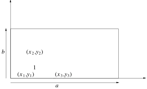
In this paper, the rectangular cross section of the waveguide is divided into a number of finite elements. An element is considered to be first order triangular in shape [3]. An schematics of a triangular finite element in the rectangular waveguide is shown in Figure 1. Consider

b

a

(x2,y2)

(x3,y3) (x1,y1)

1

Figure 1. Schematic representation of a triangular ﬁnite element. a triangle having vertices (x1, y1),(x2, y2),(x3, y3). Two vectors, −→u

and −→v has been drawn by joining the vertices [(x1, y1),(x2, y2)] and

[(x1, y1) and (x3, y3)], respectively. Let

d1 =|u|=

(x2−x1)2+ (y2−y1)2 (1)

and

d2=|v|=

(x3−x1)2+ (y3−y1)2 (2)

The unit vector along the two directions uand v are

ˆ

u= u |u| =

(x2−x1, y2−y1)

d1

(3)

and

ˆ

v= v |v| =

(x3−x1, y3−y1)

d2

(4)

any point (x, y) inside this triangle can be represented as

(x, y) = (x1, y1) +u·uˆ+v·ˆv

= (x1, y1) +

u(x2−x1, y2−y1)

d1

+v(x3−x1, y3−y1)

d2

so

(x−x1) =

u(x2−x1)

d1

+v(x3−x1)

d2

(5)

and

(y−y1) =

u(y2−y1)

d1

+v(y3−y1)

d2

(6)

These are two linear equations for the variable u and v and solving them gives us u, v as linear functions of x, y. The area measure is given by

ds(u, v) =|u×v|du·dv

where

|u×v|= sin(α)

here angleα between the vectors u and v deﬁned as

cos(α) = u·v

d1·d2

= (x2−x1)(x3−x1) + (y2−y1)(y3−y1)

d1·d2

(7)

The integral of a function can be evaluated as

I(φ) = 1 2

d1

0

d2

0

φ

x1+

u(x2−x1)

d1

+v(x3−x1)

d2

,

y1+

u(y2−y1)

d1

+v(y3−y1)

d2

sinα·dudv (8)

ifφ= 1 then we get

I(1) = d1·d2sinα

2 (9)

which represents the area of the triangle. Suppose we write

(4)

for

x, y∈∆

with ∆ as the area bounded by the triangle. a, b, c are chosen so that

V at the vertices are given, i.e.,

V(x1, y1) = V1

V(x2, y2) = V2

V(x3, y3) = V3

Thus, _

 xx12 yy12 11

x3 y3 1

 

  ab

c



=

  VV12

V3

 

Thus we ﬁnd that

a=V1(y2−y3) +V2(y3−y1) +V3(y1−y2)

∆ (10)

b=V1(x2−x3) +V2(x3−x1) +V3(x1−x2)

∆ (11)

c=V1(x2·y3−x3·y2)+V2(x3·y1−x1y3)+V3(x1·y2−x2·y1)

∆ (12)

where

∆ =x2·y3−x3·y2+x3·y1−x1y3+x1·y2−x2·y1 (13)

thus for

x, y∈∆ we have

V(x, y) = ax+by+c

= V1φ1(x, y) +V2φ2(x, y) +V3φ3(x, y)

φ1(x, y) =

(y2−y3)x+ (x2−x3)y+ (x2·y3−x3·y2)

∆ (14)

φ2(x, y) =

(y3−y1)x+ (x3−x1)y+ (x3·y1−x1·y3)

∆ (15)

φ3(x, y)) =

(y1−y2)x+ (x1−x2)y+ (x1·y2−x2·y1)

∆ (16)

(5)

ﬁrst

I1=

∆

V₍2_x,y₎dx·dy

second

I2 =

∆|∇

V|2dx·dy

Now

I1 =

∆

V₍2_{x, y}₎dx·dy=

∆

(ax+by+c)2dx·dy (17)

By substituting the value of (x, y) in terms of (xi, yi) in Equation (17), we get

I(φ) = sinα 2 d1 0 d2 0 a

x1+

u(x2−x1)

d1

+v(x3−x1)

d2

+b

y1+

u(y2−y1)

d1

+v(y3−y1)

d2

+c

2

dudv (18)

The use of method of variable separation for u and v results in the following.

I(φ) = sinα 2 d1 0 d2 0 u

a(x2−x1) +b(y2−y1)

d1

+v

a(x3−x1) +b(y3−y1)

d2 +c 2 (19) where

c =ax1+by1+c

Equation (19) can be written as

I(φ)=sinα 2 d1 0 d2 0

C1u2+C2uv+C3v2+C4u+C5v+C6

dudv(20)

Here

C1 =

_a₍_x

2−x1) +b(y2−y1)

d1

2

(21)

C2 = 2

a(x2−x1) +b(y2−y1)

d1

a(x3−x1) +b(y3−y1)

d2

(22)

C3 =

a(x3−x1) +b(y3−y1)

d2

2

(6)

C4 =

2C(a(x2−x1) +b(y2−y1))

d1

(24)

C5 =

2C(a(x3−x1) +b(y3−y1))

d2

(25)

C6 = C2 (26)

Also note that

d1

0

d2

0

u2dudv = d

3 1·d2

3 (27)

d1

0

d2

0

v2dv = d1·d

3 2

3 (28)

d1

0

d2

0

u·vdudv = d

2 1·d22

4 (29)

and ﬁnally

d1

0

d2

0

dudv=d1·d2 (30)

We also have

∇V(x, y) = (a, b) (31) and hence

I2 =

∆|∇

V|2dxdy =

a2₊_b2_d

1·d2sinα

2 (32)

Following the procedure stated above, these two integrals (I1 and I2)

for each element are evaluated. We will ﬁnd the summation of these integrals up to the number of elements in which we have divided the cross-section.

Characteristic power-voltage impedance Z can be deﬁned as follows:

Z = U

2

2P (33)

whereP is the power carried along the waveguide andU is the voltage across the waveguide.

3. DETERMINATION OF EIGENVALUES OF THE MATRIX

The eigenvalues of the matrix are obtain as follows.

(7)

when minimized over V gives the quadratic form deﬁned by

∆|∇

V|2dxdy−k2

∆

V2dxdy (34)

here

δ

∆

∇−→V ,∇−→Vdxdy= 2

∆

₋_→

∇, δ−→∇Vdxdy=−2

δV∇2V dxdy (35)

and

δ

∆

V2dxdy =

2V δV dxdy (36)

From Equation (33)

−2

δV∇2V dxdy−2k2

δV ·V dxdy= 0 (37)

or

δV

∇2₊_k2_{V dxdy} _{= 0} ₍₃₈₎

∇2₊_k2_{V dxdy} _{= 0} ₍₃₉₎

An approximation of Equation (39) using the fem gives

AV −k2BV = 0 (40)

A−k2BV = 0 (41)

|A−k2B|= 0 (42) HereV is the vector of vertex nodal ﬁeld values. Solution of this matrix will give the eigen values. These eigen values are the propagation modes of the waveguide. The above proposed method can be used to calculate the modes of a waveguide of any type of cross-section. This calculation procedure has been validated to present validity, accuracy and reliability of the solution, in the ensuing section.

4. SIMULATION RESULTS

(8)

Table 1. Eigenvalue and characteristic impedance of the fundamental mode of the rectangular waveguide.

b/a eigen value (Present)

eigen value (Theoretical)

characteristic impedance (z)

.1 1.266 1.1368 56.28

.2 1.6748 1.3475 97.42

.3 1.9717 1.8975 136.72

.4 2.2168 2.2834 173.78

.5 2.4288 2.4432 207.84

.6 2.7853 2.7582 278.44

.8 3.5839 2.9342 308.65

.9 3.8432 3.1502 342.43

1.0 3.6599 3.5422 401.87

5. CONCLUSION

In this paper an advantageous finite element method for the rectangular waveguide problem has been developed by which complex propagation characteristics may be obtained for arbitrarily shaped waveguide. The extension to higher order elements is straightforward, and by modifications of the method it is possible to treat other types of waveguides as well, e.g., dielectric waveguides with impedance walls and open unbounded dielectric waveguides properly treating the region of infinity.

ACKNOWLEDGMENT

The authors gratefully acknowledge Prof. Raj Senani for his constant encouragement and provision of facilities for this research work.

REFERENCES

1. Silvester, P. P. and R. L. Ferraro, Finite Elements for Electrical Engineers, 2nd edition, Cambridge University Press, NewYork, 1990.

(9)

non-homogeneous rectangular waveguide,” IEEE International Conference, INDICON-06, September 15–17, 2006.

3. Sadiku, M. N. O., Numerical Techniques in Electromagnetics, CRC Press, 2000.

4. Harrington, R. F.,Field Computation by Moment Methods, Series on Electromagnetic Waves, IEEE Press, 1993 (1968).

5. Jin, J. M., The Finite Element Method in Electromagnetics, 2nd edition, Wiley, NewYork, 2002.

6. Xiao, J.-K. and Y. Li, “Analysis for transmission characteristics of similarly rectangular guide ﬁlled with arbitrary-shaped inhomogeneous dielectric,”Journal of Electromagnetic Waves and Applications, Vol. 20, No. 3, 331–340, 2006.

7. Manzanares-Martinez, J. and J. Gaspar-Armenta, “Direct integra-tion of the constitutive relaintegra-tions for modeling dispersive metama-terials using FDTD technique,”Journal of Electromagnetic Waves and Applications, Vol. 21, No. 15, 2297–2310, 2007.

8. Gregorczyk, T. M. and J. A. Kong, “Reviewof left-handed metamaterials: Evolution from theoretical and numerical studies to potential applications,”Journal of Electromagnetic Waves and Applications, Vol. 20, 2053–2064, 2006.

9. Chen, H., B. I. Wu, and J. A. Kong, “Reviewof electromagnetic theory in left-handed materials,” Journal of Electromagnetic Waves and Applications, Vol. 20, No. 15, 2137–2151, 2006. 10. Singh, V., B. Prasad, and S. P. Ojha, “Modal analysis and

waveguide dispersion of an optical waveguide having a cross section of the shape of a cardioid,” Journal of Electromagnetic Waves and Applications, Vol. 20, No. 8, 1021–1035, 2006.

11. Maurya, S. N., V. Singh, B. Prasad, and S. P. Ojha, “Modal analysis and dispersion curves of an annular lightguide with a cross-section bounded by two Piet-Hein curves,” Journal of

Electromagnetic Waves and Applications, Vol. 17, 1025–1036,