Scholarship@Western
Scholarship@Western
Electronic Thesis and Dissertation Repository
8-18-2016 12:00 AM
Studying Both Direct and Indirect Effects in Predator-Prey
Studying Both Direct and Indirect Effects in Predator-Prey
Interaction
Interaction
Xiaoying Wang
The University of Western Ontario
Supervisor Zou, Xingfu
The University of Western Ontario
Graduate Program in Applied Mathematics
A thesis submitted in partial fulfillment of the requirements for the degree in Doctor of Philosophy
© Xiaoying Wang 2016
Follow this and additional works at: https://ir.lib.uwo.ca/etd
Part of the Dynamic Systems Commons
Recommended Citation Recommended Citation
Wang, Xiaoying, "Studying Both Direct and Indirect Effects in Predator-Prey Interaction" (2016). Electronic Thesis and Dissertation Repository. 3957.
https://ir.lib.uwo.ca/etd/3957
This Dissertation/Thesis is brought to you for free and open access by Scholarship@Western. It has been accepted for inclusion in Electronic Thesis and Dissertation Repository by an authorized administrator of
Studying and modelling the interaction between predators and prey have been one of the central
topics in ecology and evolutionary biology. In this thesis, we study two different aspects of
predator-prey interaction: direct effect and indirect effect.
Firstly, we study the direct predation between predators and prey in a patchy landscape. A
model where prey reside in two isolated patches and predators move between two patches to
forage prey with the strategy that maximizes their fitness is proposed. Analytical conditions of
persistence and extinction of predators are obtained. Moreover, numerical simulations indicate
that either weak or strong adaptation of predators has a stabilizing effect in predator-prey system
for certain cases. Torus bifurcation is also observed, which implies complex dynamic behaviors.
Secondly, we study indirect effects between predators and prey. Without being directly killed
by predators, prey reproduction success is largely reduced by avoidance behaviors. We propose
a model which incorporates the impact of fear effect in prey reproduction. Our model shows that
high levels of anti-predator behaviors may stabilize predator-prey system by excluding periodic
solutions while relatively low levels of anti-predator behaviors may induce Hopf bifurcation.
Moreover, the direction of Hopf bifurcation can be either supercritical or subcritical, in contrast
to the model without fear effect.
Thirdly, we extend our previous model by incorporating a stage-structure into prey. We also
assume that adult prey avoid direct predation adaptively to maximize instant growth rate of both
adults and juveniles. Mathematical analyses show that fear effect can interplay with maturation
delay between juvenile and adult prey in determining the long-term population dynamics. The
positive equilibrium may lose stability with an intermediate value of delay and regain stability if
the delay is large.
Finally, we further extend our previous model by incorporating spatial structures into
modeling. Pattern formation is studied for the model with avoidance behaviors of prey and the
cost on prey reproduction. Mathematical and numerical analyses show that either small or large
predator-taxis may induce pattern formation, depending on the form of functional response.
Keywords: Predator-prey, adaptive behavior, uniform persistence, anti-predator response,
fear effect, stability, bifurcation, delay, pattern formation.
Chapter 2: X. Wang and X. Zou (2016), On a two-patch predator-prey model with adaptive
habitancy of predators,Discrete and Continuous Dynamical Systems-Series B, 21(2), 677-697.
Chapter 3: X. Wang, L. Y. Zanette, and X. Zou (2016), Modelling the fear effect in predator-prey
interactions,Journal of Mathematical Biology, DOI 10.1007/s00285-016-0989-1, in press.
Chapter 4 is based on the paper: X. Wang and X. Zou, Modelling the fear effect in predator-prey
interactions with adaptive avoidance of predators, preprint.
Chapter 5 is based on the paper: X. Wang and X. Zou, Pattern formation of a predator-prey
model with the cost of anti-predator behaviors, preprint.
The model in Chapter 2 is formulated by X. Wang and X. Zou. The models in Chapter 3, Chapter
4, and Chapter 5 are formulated by X. Wang and X. Zou, according to discussion with L. Y.
Zanette. The mathematical analyses and numerical simulations in each of the above chapters
are performed by X. Wang under the supervision of X. Zou.
The draft of the paper in Chapter 2 is prepared by X. Wang and then revised by X. Zou.
The draft of the paper in Chapter 3 is prepared by X. Wang and then revised by L. Y. Zanette
and X. Zou.
The draft of the paper in Chapter 4 is prepared by X. Wang and then revised by X. Zou.
The draft of the paper in Chapter 5 is prepared by X. Wang and then revised by X. Zou.
At this point, firstly, I would like to express my sincere gratitude to my supervisor Dr. Xingfu
Zou. His enthusiasm for research and rigorous attitude of academics highly inspire me. Without
his helpful guidance during the past five years, countless discussions and timely responses about
research, I couldn’t make it this far on the way to pursue an academic career.
Secondly, I would like to thank all the professors and staffin the applied math department.
I have learned a lot of valuable knowledge of math and have acquired essential skills such as
programming from taking courses within the department. I have also received continuous help
from administrative staffsince I initially arrived at Western.
Thirdly, I am thankful for the companion of all my friends here, especially members in Dr.
Zou’s group, which makes my stay at Western a very enjoyable experience.
Last but not least, I thank the unconditional support and tremendous encouragement from
both my parents and my husband. I am very lucky to have such family members who respect
my decisions and support my pursuit of academic goals.
Abstract i
Co-Authorship Statement ii
Acknowledgements iii
List of Figures vii
List of Tables x
1 Introduction 1
1.1 Overview of predator-prey interaction . . . 1
1.2 Mathematical modelling of direct effects . . . 3
1.2.1 Functional responses . . . 3
1.2.2 Paradox of enrichment . . . 5
1.3 Mathematical theories and methodologies . . . 5
1.3.1 Stability analysis of equilibria . . . 6
1.3.2 Hopf bifurcation . . . 6
1.4 Thesis motivation and outline . . . 6
Bibliography . . . 8
2 On a two-patch predator-prey model with adaptive habitancy of predators 13 2.1 Introduction . . . 13
2.2 Model formulation . . . 15
2.3 Mathematical analysis . . . 17
2.4 Numerical simulations . . . 30
2.5 Conclusion and discussions . . . 31
Bibliography . . . 32
3 Modelling the fear effect in predator-prey interactions 40 3.1 Introduction . . . 40
3.4 Model with the Holling Type II functional response . . . 45
3.4.1 Existence of equilibria and dynamical behaviours in boundary . . . 45
3.4.2 Global stability of positive equilibrium . . . 48
3.4.3 Existence of limit cycles and Hopf bifurcation . . . 49
3.5 Numerical Simulations . . . 55
3.6 Conclusions and discussions . . . 57
Bibliography . . . 64
4 Modelling the fear effect in predator-prey interactions with adaptive avoidance of predators 69 4.1 Introduction . . . 69
4.2 Model formulation . . . 71
4.3 Well-posedness of the model . . . 74
4.4 Long term dynamics of the model . . . 75
4.4.1 Model with constant defense level . . . 76
4.4.2 Model with adaptive defense level—a special case: d1= 0, s1 =0 . . . 78
4.4.2.1 Equilibria of system (4.26) . . . 79
4.4.2.2 Dynamics of system (4.26) . . . 81
4.4.3 Full model . . . 89
4.5 Conclusion and discussion . . . 93
Bibliography . . . 98
5 Pattern formation of a predator-prey model with the cost of anti-predator be-haviors 102 5.1 Introduction . . . 102
5.2 Model Formulation . . . 103
5.3 Global existence of classical solution . . . 105
5.4 Pattern Formation . . . 109
5.4.1 Linear functional response . . . 110
5.4.2 The Holling-type II functional response . . . 114
5.4.3 Ratio-dependent functional response . . . 117
5.4.3.1 With density independent death rate for the predator . . . 119
5.4.3.2 With density dependent death rate for the predator . . . 123
5.4.4 Beddington-DeAngelis functional response . . . 124
6 Conclusions and discussions 134
Bibliography . . . 136
Curriculum Vitae 139
2.1 Adaptive dispersal in a favourable patch . . . 32
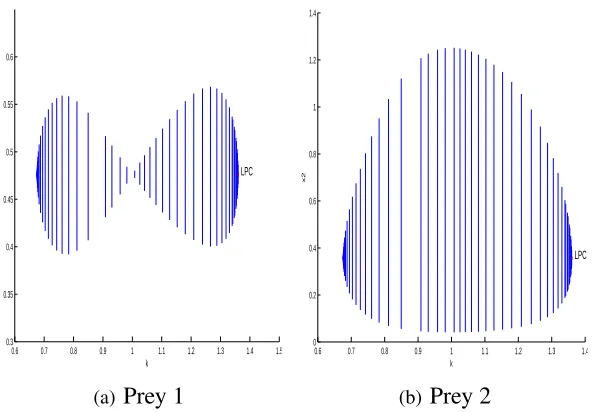
2.2 Hopf bifurcation of model (2.5) . . . 33
2.3 Periodic oscillation of x1,x2in the interval of Hopf bifurcation . . . 34
2.4 Periodic oscillation ofy,vin the interval of Hopf bifurcation . . . 34
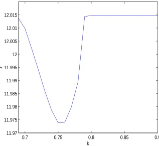
2.5 The impact ofkon average biomass ofy. . . 35
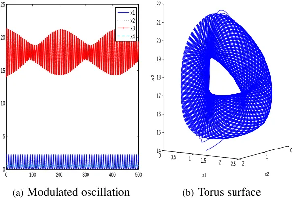
2.6 A torus surface of (2.5) . . . 36
3.1 (i) Possibility of supercritical/subcritical Hopf bifurcation . . . 53
3.2 (ii) Possibility of supercritical/subcritical Hopf bifurcation . . . 54
3.3 (iii) Possibility of supercritical/subcritical Hopf bifurcation . . . 54
3.4 Hopf bifurcation in ther0,qplane . . . 58
3.5 Supercritical Hopf bifurcation . . . 58
3.6 Subcritical Hopf bifurcation . . . 59
3.7 A bi-stable case . . . 59
3.8 Two dimensional projection of Hopf bifurcation curve whenk ,0 intok,qand k,r0 respectively. . . 60
3.9 Hopf bifurcation in ther0,pplane . . . 60
3.10 Two dimensional projection of Hopf bifurcation curve whenk, 0 intok,pand k,r0 respectively. . . 61
3.11 Hopf bifurcation in ther0,mplane . . . 61
3.12 Two dimensional projection of Hopf bifurcation curve whenk, 0. . . 62
3.13 Relationship betweenk1andk2along the Hopf bifurcation line when taking fear function (3.59). . . 62
3.14 The biomass for predators and prey from periodic solutions with varyingkdue to supercritical Hopf bifurcation. . . 63
4.1 Optimal defense level with constantα . . . 78
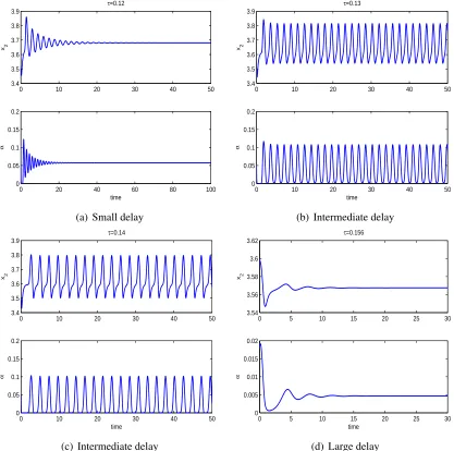
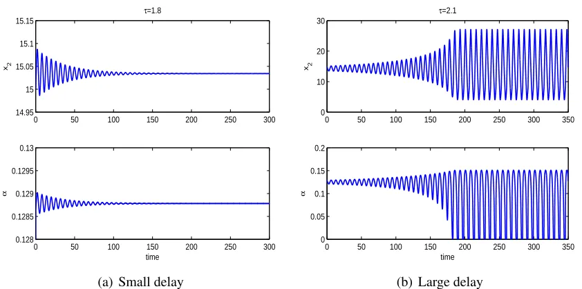
4.2 Stability switch ofEs . . . 85
4.3 Stability switch ofEswith varyingτ . . . 86
4.4 Stability switch ofEp1 where onlyEp1exists as a positive equilibrium . . . 89
4.6 Stability switch ofEp1 where bothEp1andEp2 may exist . . . 91
4.7 Stability switch ofEp1 with varyingτ . . . 91
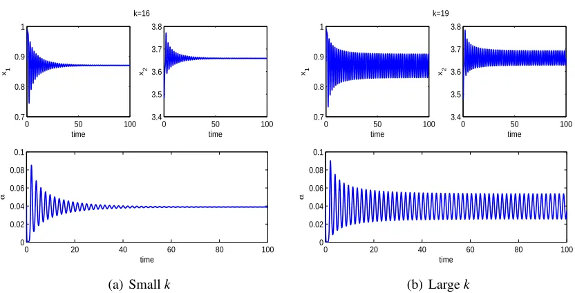
4.8 Steady state or oscillation of system (4.6) with varyingk . . . 94
4.9 Steady state or oscillation of system (4.6) with varyingb1 . . . 94
4.10 Steady state or oscillation of system (4.6) with varyingd1 . . . 95
4.11 Steady state or oscillation of system (4.6) with varyingy . . . 95
4.12 Impact ofyon the positive equilibriumEp1 . . . 96
4.13 Impact ofb1 on the positive equilibriumEp1 . . . 96
4.14 Difference between ¯x21inEp1( ¯x21,α¯1) and x+2 in (4.17) . . . 97
5.1 Conditions of global stability ofE( ¯u,v) when¯ αvaries withm(v)=m1+m2v andp(u,v)= p . . . 114
5.2 Conditions of global stability ofE( ¯u,v) when¯ k0varies withm(v)=m1+m2v andp(u,v)= p . . . 115
5.3 Spatial homogeneous steady states ofu,vwith the Holling type II functional response and density-dependent death function of predators whenαis large . . 118
5.4 Spatial heterogeneous steady states ofu,vwith the Holling type II functional response and density-dependent death function of predators whenαis small . . 118
5.5 Spatial homogeneous steady states ofu,vwhenk0 =0, αis large,m(v)=m1, andp(u,v)=b1/(b2v+u) . . . 124
5.6 Spatial heterogenous steady states ofu,vwhenk0 =0, αis small,m(v)=m1, andp(u,v)=b1/(b2v+u) . . . 125
5.7 Conditions of diffusion-taxis-driven instability ofE( ¯u,v) with changing¯ αwhen k0, 0,m(v)=m1,andp(u,v)=b1/(b2v+u) . . . 125
5.8 Spatial homogeneous steady states ofu,vwhenk0 ,0, αis small,m(v) =m1, andp(u,v)=b1/(b2v+u) . . . 126
5.9 Spatial heterogenous steady states ofu,vwhenk0 , 0, αis large,m(v) =m1, andp(u,v)=b1/(b2v+u) . . . 126
5.10 Spatial homogeneous steady states ofu,vwhenk0is small,α,0,m(v) =m1, andp(u,v)=b1/(b2v+u) . . . 127
5.11 Spatial homogeneous but temporal periodic solutionu,vover time whenm(v)= m1+m2v,k0 is large, andp(u,v)= b1/(b2v+u) . . . 127
5.12 Spatial homogeneous steady states ofu,vwhenm(v) =m1,k0 , 0, αis large, andp(u,v)= p/(1+q1u+q2v) . . . 128
= + 1 + 2
2.1 The upper indexi(i = 1,2) indicates that predators forage only in patchiwithout
migrating to the other patch.E( ˜x∗1,x˜∗2,y˜∗,v˜∗) is the unique positive equilibrium. . . 21
3.1 Direction of Hopf bifurcation by takinga6as a bifurcation parameter.
Hereai1,i = +,−are defined in (3.56), (3.57) andr1,r2are larger and smaller
roots of (3.53) respectively. . . 55
Chapter 1
Introduction
1.1
Overview of predator-prey interaction
Understanding predator-prey interaction has been one of the central topics in ecology and
conservation biology. In an ecological community, most species depend on successful
pre-dation to survive because prey serve as food resources which provide predators with energy.
Consequences of converting prey biomass into predator biomass through direct predation are
referred to as a direct effect between predators and prey, and have been the focus of modelling
predator-prey interactions ([5, 33]).
Among direct effects between predator-prey interactions, successful hunting is essential for
predators to survive as a species. Although for an individual predator, the hunting mode may
vary instantly according to changes of the surrounding environment, most species have adopted
particular hunting strategy via long-term evolution ([38]). There are two main but completely
different types of hunting strategy: one is called ambush strategy and the other one is called
active strategy ([38]). Species in an ecological community can be classified into two categories
of predators depending on their hunting mode when they forage prey. Species such as snakes
or spiders are ambush predators because their hunting strategy is “sit and wait” ([43]). When
prey approach, ambush predators trap the prey or take the opportunity to pounce on it. On the
contrary, species such as African wild dogs forage prey actively in a habitat and usually catch
prey after a relatively long-distance chase ([10]). Hence, wild dogs can be classified as active
foragers due to their active movement when foraging prey.
Because active foragers move widely in habitats when searching for prey, one natural
question is that how will the difference in landscape impact the predator-prey interaction?
Habitat fragmentation disconnects landscape and separates habitats for prey or predators into
abundance of prey. When migration or dispersal of a predator is incorporated, one interesting
question is that what is the optimal dispersal strategy for a predator? Moreover, dispersal of a
predator between patches may change the pattern of predator-prey dynamics in a single isolated
patch. For example, without dispersal of a predator, the prey and predators may tend to a steady
state in an isolated patch. However, dispersal of predators may destroy the steady state and
induce oscillations in predator or prey demography. Extensive research has been conducted
concerning patches and dispersals of predators or prey (see references [7, 8, 28, 29, 42] for
example).
Earlier research about predation behaviors and dispersal of either prey or predators assume
random dispersal of species (see e.g. [28, 29] for example). However, it has been argued that
almost all species have the ability to learn and adapt to changes of the nearby environment
([6, 40]). The adaptive behaviors of a species play an important role in determining the species’
survival and evolution by maximizing individual payoff([6, 40]). In recent years, there have
been some studies that combined the spatial dispersal of species and adaptive behaviors of
species together ([7, 8, 12, 13, 14, 27]).
Because direct effects such as direct killing of prey or migration of a species can be easily
observed in an ecological community, and have been the central topic in research by far,
indirect effects may play an even more important role in determining the demography of species.
Indirect effects between predators and prey are mainly induced by anti-predator behaviors
of prey. It has been argued by theoretical biologists that prey can perceive predation risk at
least to some extent and avoid direct killing by predators through a variety of anti-predator
behaviors ([15, 35, 36, 37, 41]). The fear of predators drives prey to show anti-predators
responses, which include habitat switch, foraging behaviors change, and increased vigilance
([9]). Specifically, when prey are in breeding season, any change of the above anti-predator
responses may lead to a loss on prey reproduction success even though no direct killing has
been involved ([9, 15, 30, 31]). Because of such decay on prey reproduction, anti-predator
behaviors may increase short-term survival rate of prey but in the long-term, there is a cost
in the fitness of prey as a species ([9]). Recently, a field study on song sparrow populations
confirms the theoretical argument that even rare presence of predators can exert a large impact
on prey demography ([45]).
In [45], a field study on song sparrows has been conducted by Zanetteet al. during the
whole breeding season. The authors in [45] eliminated all direct predation of both juvenile and
adult song sparrows by effectively using netting and electrical fences to protect nests. Without
direct predation, however, the authors used sounds of predators to manipulate predation risk.
Two groups of breeding song sparrows were monitored, within which one was exposed to
reproduction success of the two tested groups, the authors concluded that the group exposed
to predation risk reproduced 40% less offspring than the other group. In fact, the impact of
adult song sparrow’s anti-predator behaviors exist in every stage of breeding process. When
exposed to predation risk, adult song sparrows laid fewer eggs, fewer eggs were successfully
hatched and fewer nestlings survived, which all contributed to the eventual 40% loss of offspring.
Moreover, various anti-predator behaviors of adult song sparrows were observed in [45], such
as change of habitat. As indicated in [45], adult song sparrows were more willing to locate nests
in habitats with sub-optimal quality if a predation risk is persisted. On one hand, relocating
to habitats with less predation risk increases the surviving probability of adult song sparrows,
but on the other hand, it decreases the survival rate of newborn song sparrows due to less
suitable living conditions. In addition, the authors also documented that adult song sparrows
in the group exposed to predator’s sounds feed their offspring less and stayed less on brood
to protect juveniles. As a consequence, lower survival rate of nestlings was found for the
group with predation risk compared to the one without predation risk. In recent years, similar
results have also been obtained from field experiments of other vertebraes, such as birds
([17, 18, 19, 20, 24, 25, 26, 34]), elk ([11]), snowshoe hares ([39]) ,and dugongs ([44]). All
the aforementioned experiments offered evidence that the mere presence of predators could be
strong enough to impact the interaction between predators and prey. Indirect effects may play
a more important role in determining the demography of both prey and predators than direct
predation.
1.2
Mathematical modelling of direct e
ff
ects
1.2.1
Functional responses
As mentioned in the previous section, direct effects measure the conversion of prey biomass
to predator biomass through predation. Extensive and intensive research has been done about
modelling direct predation between prey and predators. One of the earliest work that modeled
direct effects between predator-prey interaction is the Lotka-Volterra predator-prey model
dx
dt = αx−βx y, dy
dt = cβx y−γy,
(1.1)
where xandyrepresents the biomass of prey and predators respectively,βis the attacking rate
of prey by predators,cis the conversion rate from prey biomass to predator biomass. One of the
called a linear functional response of the predator ([5, 33]). After the classic work of Lotka and
Volterra, Holling ([22, 23]) proposed the well-known Holling type II functional response
f(x)= βx
1+βh x (1.2)
and the Holling type III functional response ([22, 23])
f(x)= βx
θ
1+βh xθ. (1.3)
Derived from a more realistic assumption, Holling improved the linear functional response by
incorporating a predator handling time of prey besides attacking. In (1.2) and (1.3),hrepresents
predator handling time of prey, and in (1.3),θ >1 is a constant. Obviously, the Holling type III
functional response can be viewed as a generalization of the type II functional response. The
common feature of the Holling type II and type III functional responses lies in that they are
both saturating functions when the density of prey becomes large. However, the Holling type III
functional response differs from the type II functional response when prey density is at lower
level. A possible explanation is that it is more difficult for the predators to learn searching for
prey effectively if the density of prey itself is low ([22, 23]).
Although assumptions and detailed mechanisms are different for each of Holling’s functional
responses, all of the Holling type functional responses are predator-independent functional
responses. Prey-dependent functional response assumes that the predator per capita consumption
rate of prey is influenced by prey density alone. However, it is argued that the conversion of
prey biomass to predator biomass does not only depend on prey density but also depends on
predator density ([2, 3]). A well-known functional response which depends on both prey and
predator density is the Beddington-DeAngelis functional response ([4, 16])
f(x,y)= βx
1+a x+b y. (1.4)
The Beddington-DeAngelis functional response (1.4) can be regarded as a generalization of the
Holling type II functional response (1.2) by incorporating an extra termb yin the denominator.
Here, in fact, the termb ymodels the interference between predators when searching for prey. In
prey dependent only functional responses (e.g. Holling type functional responses), the encounter
between predators and prey is assumed to be random and unbiased. However, the competition
of prey or resources increases if the density of predators becomes larger. Hence, the successful
predation rate of prey by a predator decreases with increasing density of predators. Another
functional response that depends on both prey and predator densities and has been studied
extensively is the ratio dependent functional response
f(x,y)=
βx y
axy +b =
βx
The ratio-dependent functional response (1.5) is suitable when the predator is active foragers
since the predation success is an increasing function of the rate x/y, which accounts for the
average number of prey per predator can have. The function (1.5) can also be derived from
separating different time scales between behavioral change and demographical change of prey
and predators ([2, 3]). The authors of [2, 3] found empirical evidence that the ratio-dependent
functional response fitted experimental data of certain species better than prey-dependent
functional response.
Debate about whether prey dependent only functional responses or functional responses that
depend on both prey and predator densities could describe a more realistic predation behavior
has lasted for more than a decade ([1]). Due to the complexity of food webs, no explicit and
general conclusions have been recognized commonly by either theoretical or experimental
ecologists. Each type of the aforementioned functional responses has its merits and drawbacks,
and fits different situations.
1.2.2
Paradox of enrichment
Paradox of enrichment describes a phenomenon which arises from predator-prey model with
the Holling type II functional response
dx dt =r0x
1− x
K
− βx
1+βh x, dy
dt =
cβx
1+βh x −γy.
(1.6)
Gilpin et al. studied the stability of the positive equilibrium of (1.6) ([21]). By regarding
the carrying capacity K as a bifurcation parameter, Gilpinet al. find that prey and predator
densities tend to a steady state ifK is small but oscillate periodically ifK is large enough to
pass a critical value. By plotting the phase portrait of prey/predator density, it is observed that
a limit cycle exists and stays very close to both axes for a large portion of time. Therefore,
a small perturbation or stochasticity would drive prey/predator species to extinction. It is
counter intuitive because the coexistence of prey and predator should be enhanced if the carrying
capacity is large (equivalently better environment).
1.3
Mathematical theories and methodologies
This thesis uses dynamical system approach to explore the population dynamics of predator-prey
1.3.1
Stability analysis of equilibria
In dynamical system theory, equilibrium solutions are solutions which do not change with
time ([32]). Studying equilibrium solutions is important in mathematical biology because
it predicts long-term behaviors of a system. An equilibrium solution can be asymptotically
stable, which means that the equilibrium attracts trajectories in some neighborhood of the
equilibrium or unstable, meaning it repels trajectories. The stability of an equilibrium may be
local or global, depending on the basin of attraction of the equilibrium. To determine the local
stability of an equilibrium, linearization of a system at the equilibrium is an useful tool. The
equilibrium is locally asyptotically stable if all eigenvalues of the Jacbian matrix evaluated at
this point have negative real parts and is unstable if at least one eigenvalue has a positive real part
([32]). If one of the eigenvalues has zero real part, then the linearized system is not enough to
capture dynamical behaviors nearby the equilibrium and therefore, higher order approximation
is required.
1.3.2
Hopf bifurcation
Bifurcation describes an abrupt change from one state to the other when some parameters pass
the critical values. For example, water start to froze instead of keeping flowing when temperature
goes to zero. Bifurcation study is a powerful tool in understanding an ecological community
because bifurcation implies an abrupt change from one state to the other. For predator-prey
systems, the population of prey and predators may stay at a steady state or oscillate periodically.
Hopf bifurcation may be the mathematical mechanism for the change of demography of prey
and predators.
Hopf bifurcation occurs when the Jacobian matrix evaluated at an equilibrium has a pair of
pure imaginary roots crossing the imaginary axis in the complex plane, and no other eigenvalues
have zero real parts. If the pair of pure imaginary roots cross the imaginary axis with non-zero
speed, and the nondegeneracy condition is satisfied, Hopf bifurcation gives rise to a periodic
solution. A periodic solution can be stable or unstable. Typically, for Hopf bifurcation, the
stability of a bifurcated limit cycle depends on the direction of Hopf bifurcation.
1.4
Thesis motivation and outline
In this thesis, we study both direct and indirect effects in predator-prey interactions. For
direct effect, we particularly consider a case where prey reside in two isolated patches while
spatial models including patch models which incorporate dispersal of either prey or predators
have been studied extensively (see ([7, 8, 12, 13, 14, 27]) for example). The key point in our
modelling is that we consider adaptive dispersal of predators instead of random dispersal or
density-independent dispersal. In addition, by studying the combined system of both population
dynamics and adaptive dynamics, we obtain some interesting results which are induced by
dispersal of predators. More importantly, we also study indirect effects systematically, including
an ODE (ordinary differential equation) model, a DDE (delay differential equation) model,
and a PDE (partial differential equation) model, depending on the focus of modelling. By
mathematical analysis and numerical simulations, we find that indirect effects play an important
role in determining prey or/and predator demography. Under certain constraints, indirect effects
induce new dynamical behaviors of predator-prey system and may stabilize or destabilize an
equilibrium depending on the strength of anti-predator behaviors of the prey.
In Chapter2, we propose a two-patch predator-prey model where prey reside in two isolated
patches but predators move between patches to forage prey. Predators are assumed to move
adaptively between patches to maximize individual fitness. Analytical conditions of persistence
and extinction of predators are obtained. Moreover, numerical simulations show that either weak
or strong adaptation of predators stabilizes the system if the population of prey and predators
tend to a steady state in one patch but oscillate in the other. When the population of prey
and predators oscillate in both patches, torus bifurcation is identified, which implies more
complicated behaviors.
In Chapter3, we propose a model which incorporates the cost of anti-predator behaviors of
prey in the birth rate of prey. As discussed above, indirect effects induced by fear of predators (or equivalently anti-predator behaviors of prey) play an even more important role in predator-prey
interaction and thus should be modeled explicitly. Mathematical analyses show that high levels
of anti-predator responses may exclude the appearance of periodic oscillations in the
predator-prey system and thus eliminate the ‘paradox of enrichment’. However, periodic oscillations
of prey and predator demography are still possible due to Hopf bifurcation, if the level of
anti-predator response is relatively low. Different from classical model without fear effect
where Hopf bifurcation is typically supercritical, Hopf bifurcation in our model can be both
supercritical and subcritical. Subcritical Hopf bifurcation implies a case where bi-stability
exists, which shows rich dynamical behaviors. Moreover, numerical simulations show that prey
demonstrate weaker anti-predator behaviors if the birth rate of prey increases or the death rate of
predators increases, but avoid predation more strongly if the attack rate of predators increases.
In Chapter4, we extend the model in Chapter3by incorporating a stage structure of prey
into modelling. As indicated in [45], the cost of anti-predator behaviors exists through all stages
stages. Based on the experimental findings, we propose a predator-prey model with the cost
of fear and adaptive avoidance of predators. Mathematical analyses show that the fear effect
can interplay with maturation delay between juvenile prey and adult prey in determining the
long term population dynamics. A positive equilibrium may lose stability with an intermediate
value of delay and regain stability if the delay is large. Numerical simulations show that both
strong adaptation of adult prey and the large cost of fear have destabilizing effects while large
population of predators has a stabilizing effect on the predator-prey interactions. Numerical
simulations also imply that adult prey demonstrate stronger anti-predator behaviours if the
population of predators is larger and show weaker anti-predator behaviours if the cost of fear is
larger.
In Chapter5, we extend the model in Chapter3by incorporating spatial structures explicitly
into modelling. Anti-predator behaviors of prey that cause change of spatial locations such
as switch of habitat usage have been observed in experiments ([45]) and therefore should be
examined in detail. We propose and analyse a reaction-diffusion-advection predator-prey model
in which it is assumed that predators move randomly but prey avoid predation by perceiving
repulsion along predator density gradient. Based on recent experimental evidence that
anti-predator behaviors alone lead to a 40% reduction on prey reproduction rate, we also incorporate
the cost of anti-predators responses into the local reaction terms in the model. Sufficient and
necessary conditions of spatial pattern formation are obtained for various functional responses
between predators and prey. By mathematical and numerical analyses, we find that small prey
sensitivity to predation risk may lead to pattern formation if the functional response is the Holling
type II functional response or the Beddington-DeAngelis functional response but large cost of
anti-predator behaviors homogenises the system by excluding pattern formation. However, the
ratio-dependent functional response gives an opposite result where large predator-taxis may
lead to pattern formation but small cost of anti-predator behaviors inhibits the emergence of
spatial heterogeneous steady states.
We end the thesis by conclusions and discussions in Chapter6, in which a brief summary of
Bibliography
[1] P. A. Abrams and L. R. Ginzburg. The nature of predation: prey dependent, ratio dependent
or neither? Trends in Ecology&Evolution, 15:337–341, 2000.
[2] H. R. Akc¸akaya, R. Arditi, and L. R. Ginzburg. Ratio-dependent predation: an abstraction
that works. Ecology, 76:995–1004, 1995.
[3] R. Arditi and L. R. Ginzburg. Coupling in predator-prey dynamics: ratio-dependence.
Journal of Theoretical Biology, 139:311–326, 1989.
[4] J. R. Beddington. Mutual interference between parasites or predators and its effect on
searching efficiency. Journal of Animal Ecology, 44:331–340, 1975.
[5] F. N. Britton. Essential Mathematical Biology. Springer, 2012.
[6] D. M. Buss and H. Greiling. Adaptive individual differences. Journal of Personality, 67:
209–243, 1999.
[7] R. S. Cantrell, C. Cosner, D. L. Deangelis, and V. Padron. The ideal free distribution as an
evolutionarily stable strategy. Journal of Biological Dynamics, 1:249–271, 2007.
[8] R. S. Cantrell, C. Cosner, and Y. Lou. Evolutionary stability of ideal free dispersal
strategies in patchy environments. Journal of Mathematical Biology, 65:943–965, 2012.
[9] S. Creel and D. Christianson. Relationships between direct predation and risk effects.
Trends in Ecology&Evolution, 23:194–201, 2008.
[10] S. Creel and N. M. Creel. The African wild dog: behavior, ecology, and conservation.
Princeton University Press, 2002.
[11] S. Creel, D. Christianson, S. Liley, and J. A. Winnie. Predation risk affects reproductive
[12] R. Cressman and V. Kˇrivan. Migration dynamics for the ideal free distribution. The
American Naturalist, 168:384–397, 2006.
[13] R. Cressman and V. Kˇrivan. Two-patch population models with adaptive dispersal: the
effects of varying dispersal speeds. Journal of Mathematical Biology, 67:329–358, 2013.
[14] R. Cressman, V. Kˇrivan, and J. Garay. Ideal free distributions, evolutionary games, and
population dynamics in multiple-species environments. The American Naturalist, 164:
473–489, 2004.
[15] W. Cresswell. Predation in bird populations. Journal of Ornithology, 152:251–263, 2011.
[16] D. L. DeAngelis, R. A. Goldstein, and R. V. O’neill. A model for tropic interaction.
Ecology, 56:881–892, 1975.
[17] S. Eggers, M. Griesser, and J. Ekman. Predator-induced plasticity in nest visitation rates
in the Siberian jay (perisoreus infaustus). Behavioral Ecology, 16:309–315, 2005.
[18] S. Eggers, M. Griesser, M. Nystrand, and J. Ekman. Predation risk induces changes in
nest-site selection and clutch size in the siberian jay. Proceedings of the Royal Society of
London B: Biological Sciences, 273:701–706, 2006.
[19] J. J. Fontaine and T. E. Martin. Parent birds assess nest predation risk and adjust their
reproductive strategies. Ecology letters, 9:428–434, 2006.
[20] C. K. Ghalambor, S. I. Peluc, and T. E. Martin. Plasticity of parental care under the risk of
predation: how much should parents reduce care? Biology Letters, 9:20130154, 2013.
[21] M. E. Gilpin and M. L. Rosenzweig. Enriched predator-prey systems: theoretical stability.
Science, 177:902–904, 1972.
[22] C. S. Holling. The components of predation as revealed by a study of small-mammal
predation of the European pine sawfly. The Canadian Entomologist, 91:293–320, 1959.
[23] C. S. Holling. Some characteristics of simple types of predation and parasitism. The
Canadian Entomologist, 91:385–398, 1959.
[24] F. Hua, R. J. Fletcher, K. E. Sieving, and R. M. Dorazio. Too risky to settle: avian
com-munity structure changes in response to perceived predation risk on adults and offspring.
[25] F. Hua, K. E. Sieving, R. J. Fletcher, and C. A. Wright. Increased perception of predation
risk to adults and offspring alters avian reproductive strategy and performance. Behavioral
Ecology, 25:509–519, 2014.
[26] J. D. Ib´a˜nez- ´Alamo and M. Soler. Predator-induced female behavior in the absence of
male incubation feeding: an experimental study. Behavioral Ecology and Sociobiology,
66:1067–1073, 2012.
[27] V. Kˇrivan. The lotka-volterra predator-prey model with foraging–predation risk trade-offs.
The American Naturalist, 170:771–782, 2007.
[28] Y. Kuang and Y. Takeuchi. Predator-prey dynamics in models of prey dispersal in two-patch
environments. Mathematical Biosciences, 120:77–98, 1994.
[29] S. A. Levin. Dispersion and population interactions. The American Naturalist, 108:
207–228, 1974.
[30] S. L. Lima. Nonlethal effects in the ecology of predator-prey interactions. Bioscience, 48:
25–34, 1998.
[31] S. L. Lima. Predators and the breeding bird: behavioral and reproductive flexibility under
the risk of predation. Biological Reviews, 84:485–513, 2009.
[32] J. D. Meiss. Differential dynamical systems, volume 14. SIAM, 2007.
[33] J. D. Murray. Mathematical Biology, I, An Introduction. Springer, 2002.
[34] J. L. Orrock and R. J. Fletcher. An island-wide predator manipulation reveals immediate
and long-lasting matching of risk by prey. Proceedings of the Royal Society of London B:
Biological Sciences, 281:20140391, 2014.
[35] S. D. Peacor, B. L. Peckarsky, G. C. Trussell, and J. R. Vonesh. Costs of predator-induced
phenotypic plasticity: a graphical model for predicting the contribution of nonconsumptive
and consumptive effects of predators on prey. Oecologia, 171:1–10, 2013.
[36] N. Pettorelli, T. Coulson, S. M. Durant, and J-M Gaillard. Predation, individual variability
and vertebrate population dynamics. Oecologia, 167:305–314, 2011.
[37] E. L. Preisser and D. I. Bolnick. The many faces of fear: comparing the pathways and
[38] I. Scharf, E. Nulman, O. Ovadia, and A. Bouskila. Efficiency evaluation of two competing
foraging modes under different conditions. The American Naturalist, 168:350–357, 2006.
[39] M. J. Sheriff, C. J. Krebs, and R. Boonstra. The sensitive hare: sublethal effects of predator
stress on reproduction in snowshoe hares. Journal of Animal Ecology, 78:1249–1258,
2009.
[40] J. E. R. Staddon. Adaptive behavior and learning. CUP Archive, 1983.
[41] T. O. Svennungsen, Ø. H. Holen, and O. Leimar. Inducible defenses: continuous reaction
norms or threshold traits? The American Naturalist, 178:397–410, 2011.
[42] W. Wang and Y. Takeuchi. Adaptation of prey and predators between patches. Journal of
Theoretical Biology, 258:603–613, 2009.
[43] D. K. Wasko and M. Sasa. Food resources influence spatial ecology, habitat selection,
and foraging behavior in an ambush-hunting snake (Viperidae: Bothrops asper): an
experimental study. Zoology, 115:179–187, 2012.
[44] A. J. Wirsing and W. J. Ripple. A comparison of shark and wolf research reveals similar
behavioral responses by prey. Frontiers in Ecology and the Environment, 9:335–341, 2011.
[45] L. Y. Zanette, A. F. White, M. C. Allen, and M. Clinchy. Perceived predation risk reduces
Chapter 2
On a two-patch predator-prey model with
adaptive habitancy of predators
2.1
Introduction
Foraging behaviour is a common phenomenon in nature. As indicated in [19], foraging behaviour
varies from ambush to active, in response to changes in environment and other circumstances.
Although the foraging mode for a certain individual may change from time to time, many
species have adopted the most advantageous foraging strategy through long-term evolution,
either ambush or active, to maximize their survival probability. Species like spiders, or snakes,
as indicated in [25], are classified as ambush predators because they “sit and wait” and then
pounce when the opportunity arises. In contrast, other species, like wild dogs, as described in
[6], move actively to forage prey.
Active foragers move back and forth searching for prey. Foraging behaviour of predators
does not depend only on intra-species competition, but also depends on spatial abundance of
resources and interspecies interaction in different patches. It has been widely observed in nature
that many species migrate between different patches to search for resources because of apparent
differences of resources, landscapes, or other environmental factors that affect the predators’
survival probability in different patches. Consequently, patch models have been introduced to
simulate predator-prey dynamics with active foraging behaviour and dispersal of predators, as
indicated in [3, 4, 16, 17].
Patch models with dispersal of certain species have been studied extensively, see, e.g.,
[3, 4, 16, 17, 24] and the references therein. The common point in [16] and [17] is the
assumption of density-independent dispersal rates. However, more and more experimental
a better patch in which they can gain more fitness. Predators are more likely to move between
different patches adaptively.
In behavioural ecology, an adaptive behaviour is a behaviour which contributes directly or
indirectly to an individual’s survival or reproductive success and is thus subject to the forces of
natural selection ([22]). Adaptations are commonly defined as evolved solutions to recurrent
environmental problems of survival and reproduction ([2]). Ecological species have the ability
to adapt through learning ([21]). An individual will adjust its behaviour or strategy by learning
in response to a change of the environment in order to survive and acquire the highest payoff.
In evolutionary biology, analyzing an evolutionary stable strategy (ESS) under adaptation is
one of the central topics. Another important concern is how species distribute themselves
among different patches under adaptive dispersal. Based on the assumption that each individual
has the ability to assess the condition of different patches and can move freely to maximize
the individual fitness, the ideal free distribution (IFD) is proposed to illustrate the ecological
equilibrium under adaptive dynamics ([3, 10]). It is natural to analyze the relationship between
the ecological equilibrium and the evolutionary stable strategy. Several papers of [3, 4, 7, 9, 14]
studied a variety of models including a single-species model, a two-patch competition model, a
two-patch predator-prey model and an interacting-species model within finitely-many patches.
They conclude that under certain conditions and assumptions, the evolutionary stable strategies
are those which lead to the ideal free distribution.
In addition to the evolutionary and ecological aspects, predation behaviour can also produce a
significant effect on predator-prey systems. As indicated in [1], different behaviour mechanisms
can result in surprisingly different outcomes. Behavioural dynamics exerts significant effect
on ecological and evolutionary dynamics. Functional responses are used to connect different
behavioural dynamics of prey and predators. One important functional response which connects
prey density and prey catch-per-predator is the Holling type II functional response, which was
proposed by Holling ([13]). In contrast to the classical linear functional response, the Holling
type II functional response assumes that the encounter rate of prey by predators is
density-dependent. This matches experimental data for many species very well, as indicated in [5, 20].
Seitzet al. ([20]) conducted a series of experiments to study predator-prey dynamics of
thin-shelled clams and their predators, the blue crabs, which inhabit the Chesapeake Bay. As indicated
in [20], the predation onMya arenaria(soft-shell clam) in mud andM. mercenaria(hard clam)
in sand by their major predators, the blue crabs, obeys the Holling type II functional response.
Clarket al. ([5]) conducted another experiment about foraging behaviour of the blue crabs in
the Chesapeake Bay, but focused on studying the mechanism of foraging behaviour of the blue
crabs between patches. In addition to predation of clams by the blue crabs in the Chesapeake
as predation behaviour of rotifers on sessile planktonic species, and grazing behaviour of large
herbivores. The above biological instances share one feature in common: all predators are
mobile and migrate between different patches to forage prey or resources while prey or resources
are sessile. In addition, as mentioned above, foraging behaviour of predators is adaptive because
predators try to maximize individual fitness.
Kˇrivan and Cressman ([15]) studied fast behaviour of predators moving between patches
and showed that there exists a complicated relationship involving behavioural, population and
evolutionary dynamics by studying three different predator-prey models. Their study is based
on the assumption that the behavioural dynamics runs on a much faster time scale than the
demographical time scale and thus simplifies the original system. Kˇrivan and Cressman ([15])
also explored the effect of adaptive dispersal exerting on population dynamics by using computer
simulations. Based on [15], we consider a two-patch predator-prey model where predators move
between two patches foraging on prey freely but each individual of the prey resides only within
one patch. We combine population dynamics and behavioural dynamics together and investigate
detailed dynamics of the whole system under the effect of adaptive dispersal.
The rest of the paper is organized as follows. In Section 2, we present the two-patch
predator-prey model with the Holling type II functional response and adaptive dispersal of predators. In
Section 3, mathematical analysis of the model is carried out to provide analytical conditions
for persistence and extinction of the predators. Section 4 contains some numerical simulations.
One interesting observation from these simulations is that if under isolation, the populations of
the prey and predators in one patch tend to an equilibrium but those in the other patch tend to a
limit cycle, then either weak or strong adaptation of the predators may stabilize the system in
the sense that populations in both patches will tend to an equilibrium. Moreover, the strength
of adaption has influences on the average biomass of predators. When the populations of the
prey and predators tend to limit cycles in both patches under isolation, adaptive dispersal of
predators may results in torus bifurcation. In Section 5, we summarize our findings and discuss
some possible future projects along this line.
2.2
Model formulation
Our model will be built upon a two-patch predator-prey model with the Holling type II functional
response, which is also known as the Rosenzweig-MacArthur model. This model is based on
the assumptions that (i) prey and predators inhabit two patches which are totally separated; (ii)
an individual of the prey does not disperse between the two patches and only predators move
between two patches to forage on prey; (iii) the predators, they have the complete knowledge
is measured by the per capita growth rate of predators. Under these assumptions, the
two-patch Rosenzweig-MacArthur model is given by the following system of ordinary differential
equations
dx1
dt = x1(r1−a1x1)−
s1x1v y
1+h1s1x1
,
dx2
dt = x2(r2−a2x2)−
s2x2(1−v)y
1+h2s2x2
, (2.1)
dy
dt = y −m1v−m2(1−v)+
s1x1e1v
1+h1s1x1
+ s2x2e2(1−v)
1+h2s2x2
!
,
where x1 denotes the density of prey in patch 1, x2 denotes the density of prey in patch 2,y
represents the density of predators,v is the proportion of time that predators stay in patch 1
on average,ri fori = 1,2, is the intrinsic growth rate of prey in patchi,ri/ai is the carrying
capacity of prey in patchi,si is the attacking rate of the predators in patchi,eiis the expected
biomass of prey converted to predators in patchi,miis the per capita mortality rate of predators
in patchi, andhi is the handling time of the predation in patchirespectively.
In model (2.1), the proportional time vthat predators spend in patch 1 is assumed to be
constant. However, predators seem to choose their habitat intelligently according to resource
abundance in patches. In other words, they migrate between patches adaptively with the change
of surrounding environment. Ifv increases, prey in patch 1 will be reduced due to the high
predation risk and meanwhile, intra-specific competition of predators will be increased. As a
consequence, predators tend to migrate to the second patch in order to maximize energy intake.
Consequently, aggregation of predators in the second patch will again cause prey reduction in
this patch, and this in turn impels predators to migrate to the first patch. Through adaptation of
predators,vin model (2.1) should change with time rather than remain as a constant. Thusv
can be viewed as the strategy of predators.
We now derive the strategy equation based on [10] and the idea of the replicator dynamics.
As indicated in [10], the assumption that predators have the complete knowledge about patch
qualities and always tend to move to a better patch to gain more fitness is valid. Let
f1 =−m1+
e1s1x1
1+h1s1x1
, f2= −m2+
e2s2x2
1+h2s2x2
,
which measures the fitness of predators in patches 1 and 2 respectively. Because the proportion
of time that predators forage in patch 1 is v and the corresponding proportion of time that
predators stay in patch 2 is 1−v, theaverage fitnessof predators switching over the two patches
is
By the theory of adaptive dynamics ([12]), we have
dv dt =k v
f1− f
. (2.3)
By plain language, this means that the relative change rate ofvis proportional to the difference
of the fitness in patch 1 and the mean fitness over the two patches. In equation (2.3), kis a
positive constant, with largekaccounting for strong (fast) adaptation of predators in response to
a change of prey abundance in the local patch, while smallkexplaining weak (slow) adaptation
of predators.
Plugging (2.2) into (2.3), we obtain
dv
dt = k v(1−v) (f1− f2)
= k v(1−v) −m1+m2+
e1s1x1
1+h1s1x1
− e2s2x2 1+h2s2x2
!
. (2.4)
Combining (2.1) and (2.4), we obtain our model system which describes both population
dynamics and adaptive dynamics:
dx1
dt = x1(r1−a1x1)−
s1x1v y
1+h1s1x1
,
dx2
dt = x2(r2−a2x2)−
s2x2(1−v)y
1+h2s2x2
,
dy
dt = y −m1v−m2(1−v)+
s1x1e1v
1+h1s1x1
+ s2x2e2(1−v)
1+h2s2x2
!
, (2.5)
dv
dt = k v(1−v) −m1+m2+
e1s1x1
1+h1s1x1
− e2s2x2 1+h2s2x2
!
.
In the next section, we will analyze this model system.
2.3
Mathematical analysis
We first address the well-posedness of the model (2.5), including non-negativity and
bounded-ness of solutions. Since (2.5) is of Gauss type, the solution with any set of non-negative initial
values for the four unknowns will remain non-negative for allt at which the solution exists.
Moreover, if x1(0) = 0, then x1(t) = 0 for all t ≥ 0. The same conclusion also holds for all
other unknowns. For the strategy variablev(t), writing the last equation in (2.5) as the following
integral form
v(t)=1−1/ 1+v(0)/(1−v(0)) exp
(Z t
0
ψ(ξ)dξ
)!
where
ψ(ξ)=k−m1+m2+(e1s1x1(ξ))/(1+h1s1x1(ξ))
−(e2s2x2(ξ))/(1+h2s2x2(ξ))
. (2.7)
From (2.6), we know thatv(t) ∈ [0,1] fort ≥ 0, as long asv(0) ∈ [0,1]; if the casev(0) = 0
then v(t) = 0 for all t ≥ 0; ifv(0) = 1 then v(t) = 1 for t ≥ 0; and if v(0) ∈ (0,1) then so
is v(t) for allt ≥ 0. Although the dedicated cases v(0) = 0 andv(0) = 1 will be addressed
for mathematical purpose, we are mainly interested in the case of v(0) ∈ (0,1). This can
be justified by assuming that initially there are predators in both patches. Next, we address
boundedness of solutions. To this end, let (x1(t),x2(t),y(t),v(t)) be any non-negative solution
with x1(0) ≥ 0, x2(0) ≥ 0, y(0) ≥ 0 and v(0) ∈ [0,1]. We have seen from the above that
v(t)∈[0,1] for allt ≥0 where the solution exists. We only need to confirm the boundedness of
x1(t), x2(t) andy(t). To this end, letG =e1x1+e2x2+y. By direct calculation, we obtain
dG
dt =−m1v G−m2(1−v)G+[e1r1+m1v e1+m2(1−v)e1]x1
+[e2r2+m1v e2+m2(1−v)e2]x2−e1a1x12−e2a2x22
≤ −m1v G−m2(1−v)G+
[e1r1+m1v e1+m2(1−v)e1]2
4e1a1
+ [e2r2+m1v e2+m2(1−v)e2]2
4e2a2
.
(2.8)
Because we have shown thatvis bounded between 0 and 1, we obtain
dG
dt ≤ −m0G+η0, (2.9)
wherem0 =min{m1,m2}andη0is a positive constant. By the comparison principle, we conclude
that
lim sup
t→∞
G(t)= η0 m0
,
implying thatGis bounded. This also indicates thatη0/m0e1, η0/m0e2 andη0/m0 are alsoa
prioribounds ofx1(t), x2(t) andy(t) respectively. The boundedness of the solution also implies
that it exists globally, that it, it exists for allt∈(0,∞). The above analysis also show that the set
X =R4+={(x1,x2,y,v) : x1 ≥ 0,x2 ≥0,y≥ 0,0≤v≤ 1},
In order to analyze the long-term behaviour of system (2.5), we first discuss the structure of
all possible equilibria for this system. For convenience of notations, we let
A1 =
e1s1r1
a1+h1s1r1
−m1, A2=
e2s2r2
a2+h2s2r2
−m2,
A3 =e2, A4= e2−m2h2, A5 =r2s2, A6 =a2m2,
A7 =e1, A8= e1−m1h1, A9 =r1s1, A10 =a1m1.
(2.10)
Denote
x∗1 = m1
s1(e1−m1h1)
, y∗1 = e1(r1s1e1−r1s1h1m1−a1m1) s21(e1−m1h1)2
,
x∗2 = m2
s2(e2−m2h2)
, y∗2 = e2(r2s2e2−r2s2h2m2−a2m2) s22(e2−m2h2)2
.
(2.11)
Then, direct calculations show that there are always eight equilibria for the biologically
mean-ingful parameters:
E20 = (0,0,0,0), E21 = r1 a1
,0,0,0
!
, E22= 0, r2 a2
,0,0
!
, E32= r1 a1
, r2
a2
,0,0
!
,
E10 = (0,0,0,1), E11 = r1 a1
,0,0,1
!
, E21= 0, r2 a2
,0,1
!
, E31= r1 a1
, r2
a2
,0,1
!
.
In addition, five other equilibria including a unique positive equilibrium may come into existence
under certain conditions on the model parameters:
E14 = (x∗1,0,y1∗,1), E51 x∗1, r2 a2
,y∗1,1
!
,
E24 = (0,x∗2,y∗2,0), E52= r1 a1
,x∗2,y∗2,0
!
,
E∗ =( ˜x∗1,x˜∗2,y˜∗,v˜∗) with ˜x∗1 >0, x˜∗2 > 0, y˜∗> 0, v˜∗∈(0,1).
Obviously, y∗
1 > 0 if and only ifA1 > 0 which impliesA8 > 0 (hence x
∗
1 > 0). Similarly,
y∗2 >0 if and only ifA2 >0 which impliesA4 >0 (hencex∗2 >0). Here, all equilibria, except for
E∗, have explicit formulas and each represents one situation of the specialist strategies (v=0 or
v=1) meaning that all predators choose to inhabit in one patch. However,E∗with ˜v∗ ∈(0,1)
represents a generalist strategy, which can not be obtained explicitly; indeed, its existence will
be established by an argument using abstract persistence theory.
The stability/instability of these equilibria can be analyzed by the standard method of
investigating the characteristic equation at each of them, except forE∗. Below, we showcase the
analysis onE2 5.
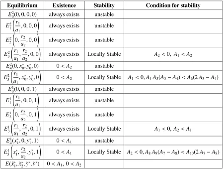
Theorem 2.3.1 Assume that A2 >0so that E25 exists. Then, it is locally asymptotically stable if
and only if
Proof The Jacobian matrix of (2.5) is
J11 0 −
s1x1v
1+h1s1x1
− s1x1y 1+h1s1x1
0 J22 −
s2x2(1−v)
1+h2s2x2
s2x2y
1+h2s2x2
e1v s1y
(1+h1s1x1)2
e2 (1−v)s2y
(1+h2s2x2)2
J33 J34
k v(1−v)e1s1
(1+h1s1x1)2
−k v(1−v)e2s2 (1+h2s2x2)2
0 J44
, (2.13) where
J11= r1−2a1x1−
s1v y
(1+h1s1x1)2
,
J22= r2−2a2x2−
s2(1−v)y
(1+h2s2x2)2
,
J33= −m1v−m2(1−v)+e1v
s1x1
1+h1s1x1
+e2(1−v)
s2x2
1+h2s2x2
,
J34= y
−m1+m2+
e1s1x1
1+h1s1x1
− e2s2x2 1+h2s2x2
,
J44= k(1−2v)
−m1+m2+
e1s1x1
1+h1s1x1
− e2s2x2 1+h2s2x2
.
Substituting equilibriumE52into the Jacobian matrix (3.26) gives the characteristic equation at
E25 :
(λ+r1)
λ− J44 λ2− J22λ−J23J32
=0, (2.14)
where
J44 =k −m1+m2+
e1s1r1
a1+h1s1r1
− e2s2x ∗
2
1+h2s2x∗2
!
,
J22 =r2−
2a2m2
s2(−m2h2+e2)
− s2y
∗
2
1+h2s2x∗2
2,
J23 =−
s2x∗2
1+h2s2x∗2
, J32 =
e2s2y∗2
1+h2s2x∗2
2.
Obviously,λ1 =−randλ2 =J44are real roots of (2.14), and the other two roots of (2.14) are
determined by the quadratic equation:
λ2−
J22λ− J23J32= 0. (2.15)
Note that J23J32 < 0. Thus, the two roots of (2.15) have negative real parts if and only if
J22< 0. Therefore, all roots of (2.14) have negative real parts if and only if
which are, by the notations defined in (2.11), equivalent to the two conditions in (2.12). This
completes the proof.
Equilibrium Existence Stability Condition for stability
E02(0,0,0,0) always exists unstable
E12 r1 a1
,0,0,0
!
always exists unstable
E22 0, r2 a2
,0,0
!
always exists unstable
E2 3
r1
a1
, r2
a2
,0,0
!
always exists Locally Stable A2<0, A1<A2
E42(0,x∗0,y∗0,0) 0<A2 unstable
E52 r1 a1
,x∗0,y∗0,0
!
0<A2 Locally Stable A1 <0,A4A5(A3−A4)<A6(2A3−A4)
E1
0(0,0,0,1) always exists unstable
E11 r1 a1
,0,0,1
!
always exists unstable
E1 2 0,
r2
a2
,0,1
!
always exists unstable
E31 r1 a1
, r2
a2
,0,1
!
always exists Locally Stable A1 <0, A2<A1
E41(x∗
1,0,y
∗
1,1) 0<A1 unstable
E51 x∗1, r2 a2
,y∗1,1
!
0<A1 Locally Stable A2 <0,A8A9(A7−A8)< A10(2A7−A8)
E( ˜x∗
1,x˜
∗
2,y˜
∗,v˜∗) 0< A
1, 0<A2
Table 2.1: The upper indexi(i=1,2) indicates that predators forage only in patchiwithout migrating
to the other patch. E( ˜x∗1,x˜2∗,y˜∗,v˜∗) is the unique positive equilibrium.
The analysis of stability/instability of other equilibria, except forE∗, can be similarly done and will be omitted here since it would cost too much space. Table 2.1 summarizes such results.
As mentioned before, the existence ofE∗can not established through solving the equations
for equilibria. Instead it is established as a result of uniform persistence of the model. To this
end, we will first establish the uniform persistence of the population with a generalist strategy
(v∈(0,1)) under the conditionsA1> 0 andA2 >0. For this purpose, we need to obtain some
information about the patch-wise dynamics, that is, the population dynamics when the predator
v=1 in (2.5)): dxi
dt = xi(ri−aixi)−
sixiy
1+hisixi
,
dy
dt =y −mi+ei
sixi
1+hisixi
!
.
(2.16)
For such a classic prey-predator model, generally, when the carrying capacity of the prey is not
too large, the populations of prey and predator tend to a unique positive steady state; while when
the carrying capacity of the prey is sufficiently large, oscillations will occur and the populations of prey and predators tend to a globally stable limit cycle. To state this more precisely, we first
note that fori=1,2,Ai > 0 is equivalent to
mihi
sihi(ei−mihi)
< ri
ai
,
which is also the condition forx∗i andy∗i to be positive (hence existence of positive equilibrium
(x∗i,y∗i) for (2.16)). Thus, if both A1andA2 are negative, regardless of whether choosing to stay
in patch 1 (v(t) =1) or patch 2 (v(t) =0), the predator will go to extinction. Indeed, in such
a case, this conclusion remains true for any general strategies in (2.5), as is confirmed in the
following theorem.
Theorem 2.3.2 The predators go to extinction if A1 <0and A2 <0.
Proof Applying the comparison principle to the first and the second equation in (2.5), we have
the estimates:
lim sup
t→∞
xi(t)≤
ri
ai
, i=1,2. Thus, for any >0, there existst∗> 0 such that
xi(t)≤
r1
a1
+ for t≥t∗. (2.17)
This together with the third equation in (2.5) lead to
dy
dt ≤ By, (2.18)
where
B= −m1v−m2(1−v)+
e1v s1(r1+a1)
a1+h1s1(r1+a1)
+ e2(1−v)s2(r2+a2)
a2+h2s2(r2+a2)
.
Noting that
lim
→0 −m1v−m2(1−v)+
e1v s1(r1+a1)
a1+h1s1(r1+a1)
+ e2(1−v)s2(r2+a2)
a2+h2s2(r2+a2)
!
=v(A1−A2)+A2 = vA1+(1−v)A2< 0.
(2.19)
One can choose >0 sufficiently small such that B< 0. This together with (2.18) implies that
By this theorem, in order for the predators to be persistent, at least one of the two quantities
A1 andA2 must be positive. To proceed further, we need the following lemma, which can be
easily proved by standard methods (see, e.g., [18]), on the prey-predator model (2.16).
Lemma 2.3.3 Assume that Ai >0. If
(Hi)
ri
ai
< ei+mihi
sihi(ei−mihi)
,
then, every positive solution of (2.16)approaches to a positive equilibrium; and if
(H−i ) ei+mihi
sihi(ei−mihi)
< ri
ai
,
then, every positive solution of (2.16)tends to a positive limit cycle, except for those solutions
starting from unstable equilibria.
In the remainder of this section, we consider the case when both A1andA2are positive, and
will leave the case thatA1A2 < 0 to the next section for discussion where we will present some
numerical simulation results.
Now we are in the position to establish the persistence of the predators, as well as of the
strategy functionsv(t) and 1−v(t) for the case when bothA1andA2are positive.
Theorem 2.3.4 Assume that A1 >0and A2> 0. Then the predator population in system(2.5)
is uniformly persistent.
Proof We apply the theory in [11, 23] to complete the proof. To this end, we distinguish four
cases:
(I) (H1) and (H2) hold; (II) (H1) and (H−2) hold;
(III) (H1−) and (H2) hold; (IV) (H1−) and (H
−
2) hold.
We only give the proof for Case (I), since the proofs for the other three cases are similar and are
thus omitted to save space.
Define
X = {(x1,x2,y,v) : x1 ≥0,x2 ≥0,y≥0,0≤v≤1},
X0 = {(x1,x2,y,v) : x1 ≥0,x2 ≥0,y>0,0≤v≤1}, (2.20)
Y = X/X0= {(x1,x2,y,v) : x1 ≥0,x2 ≥0,y=0,0≤v≤1}.
There are eight equilibria in setY:
E02(0,0,0,0), E21 r1 a1
,0,0,0
!
, E22 0, r2 a2
,0,0
!
, E32 r1 a1
, r2
a2
,0,0
!
,
E01(0,0,0,1), E11 r1 a1
,0,0,1
!
, E12 0, r2 a2
,0,1
!
, E31 r1 a1
, r2
a2
,0,1
!
Following notations in [11],A∂ being the global attractor in the boundary setY, we have
e
A∂ = ∪
x∈A∂ω(x)
= ∪Eij, i=0,1,2,3, j=1,2.
In order to show Ae∂ is isolated and has an acyclic covering, first, we consider the system
restricted onY:
dx1
dt = x1(r1−a1x1), dx2
dt = x2(r2−a2x2), (2.21)
dv
dt = kv(1−v) −m1+m2+
e1s1x1
1+h1s1x1
− e2s2x2 1+h2s2x2
!
.
Note that among equilibria Eij for i = 0,1,2,3; j = 1,2, the sequence Ei2, i = 0,1,2,3
correspond tov= 0 and the sequenceE1
i, i = 0,1,2,3 correspond tov= 1. First, we show
the analysis for the former case. When v = 0, the three-dimensional system (2.21) reduces
to a two-dimensional system. Because equilibrium E2
3 is globally asymptotically stable for
the two-dimensional system, it is clear thatE2
0,E 2 1,E
2 2,E
2
3 are isolated and acyclic in setY. By
checking eigenvalues of each equilibrium, it can be shown thatE2
0,E 2 1,E
2 2,E
2
3 are also isolated
in setX.
Next, we show thatWs(E2
3)∩X0 =∅. Suppose this is not true. Then there exists a solution
of (2.5) withy(t) positive such that
lim
t→∞(x1(t),x2(t),y(t),v(t))= r1
a1
, r2
a2
,0,0
!
. (2.22)
Denote
R(t)= −m1v−m2(1−v)+
e1v s1x1
1+h1s1x1
+ e2(1−v)s2x2
1+h2s2x2
.
Then (2.22) implies thatR(t)→A2 > 0 as→ ∞. Thus, for ∈(0,A2), there existsT >0 such
thatR(t)>A2− > 0 fort≥T. Therefore,
dy
dt = R(t)y≥(A2−)y, for t≥T, (2.23)
which implies that y grows unboundedly by the comparison principle. This contradicts the
boundedness ofy(t). Therefore,Ws(E2
3)∩X0= ∅ifA2 >0.Similarly, we can proveW
s(E2
i)∩
X0 =∅fori= 0,1,2 when conditionA2 >0 holds.
For the case corresponding tov=1, we can prove thatA1 >0 impliesWs(E1i)∩X0 =∅for
i=0,1,2,3. The proof here is similar to the proof for the casev=0 (it is actually a result of