Thesis by
Gideon Nave
In Partial Fulfillment of the Requirements for the degree of
PhD
CALIFORNIA INSTITUTE OF TECHNOLOGY Pasadena, California
© 2016 Gideon Nave
ORCID: 0000-0001-6251-5630
staff, especially Barbara Estrada, Tanya Owen, Laurel M. Auchampaugh and Tiffany Kim gave me the essential peace of mind to make my research happen.
There is a seemingly endless list of colleagues and friends who greatly contributed (and continue to contribute) to my personal and professional development. I am thankful for many hours of conversation with Juri Minxha, who has been my room-mate during my first three years at Caltech. I was fortunate to have a friend like Juri, who has the rare combination of sharp intelligence, frank sensitivity and lightness. I was blessed with many new friends who have also turned into superb research collaborators during my time at Caltech. Three of them remarkably contributed to this dissertation. Chapter 2 is the fruit of a my work with Cary Frydman, whose last year of grad school overlapped with my first year one. I was fortunate to share an office with Alec Smith. I have learned a great deal of Econometrics and Game Theory by merely sitting with Alec in the same room, and chapter 3 is the fruit of our close collaboration with Colin. The friendships of Cary and Alec greatly helped me to navigate through the loneliness and difficulties of moving from the busy streets of Tel-Aviv to the lively but unwalkable City of Angels.
Chapter 2 of my dissertation is the first product of a joint research program with Amos Nadler. Although Amos and I grew up just a few blocks from each other in Ahuza neighborhood in Haifa, we met for the first time only a few years ago. Amos was especially fun to work with, and he taught me a great deal about conducting hormonal studies.
with high cortisol and estradiol levels. These findings suggest a unified mechanism underlying testosterone’s varied behavioral effects in humans and provide novel, clear, and testable predictions.
PUBLISHED CONTENT AND CONTRIBUTIONS
4.4 Experiment . . . 101
4.5 Results . . . 104
4.6 Using process data . . . 112
4.7 Conclusion . . . 117
Appendices . . . 120
4.A Mathematical Appendix . . . 120
4.B Pooling data . . . 125
4.C List of process features and associated marginal effects . . . 127
4.D instructions . . . 130
Bibliography . . . 132
Chapter V: Conclusion . . . 139
LIST OF TABLES
Number Page
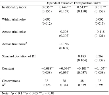
2.1 OLS regression of extrapolation index (EI) on the irrationality index
(II) and controls. . . 30
2.2 Individual differences in PDT predict behavior in EDT. . . 35
2.3 Mixed model linear regression, PDT response times (correct) . . . . 42
2.4 Mixed model logistic regression, PDT accuracy . . . 43
2.5 Mixed model linear regression, PDT response times (incorrect) . . . 43
2.6 Mixed model linear regression, EDT beliefs . . . 44
3.1 math task question example. . . 64
3.2 Demographic data summary . . . 70
3.3 Detection levels, precision and normality tests of hormonal assays . . 71
3.4 Hormone panel data measurements . . . 74
3.5 Positive and negative affect (PANAS-X) summary statistics . . . 74
3.6 CRT regression table 1 . . . 76
3.7 CRT regression table 2 . . . 77
3.8 CRT regression table 3 . . . 78
3.9 CRT score response frequencies and statistics by question . . . 79
3.10 CRT dual hormone interactions regression table . . . 81
3.11 CRT response times regression analysis . . . 83
4.1 Average payoffs and deal rates by pie size . . . 104
4.2 Logistic regression - simple predictors of deals . . . 111
4.3 Session information . . . 126
4.4 Average payoffs (case of deal) and deal rates by pie size, Caltech vs. UCLA . . . 126
C h a p t e r 1
INTRODUCTION
A multi-disciplinary effort has led to impressive progress in the field of decision neuroscience (Neuroeconomics) over the past decade (Glimcher and Fehr, 2013). It remains to be seen whether new discoveries in the field will translate into major contribution to the disciplines from which it has emerged. More specifically, there’s a need to evaluate how promising findings about the neuroscience of decision-making can inform traditional questions in economics that historically have been investigated using choice data alone and without delineating the mechanism of choice.
An optimistic view describing the potential contribution of "opening the black box" of the human mind to standard economics is described by C. Camerer, Loewenstein, and Prelec, 2005; C. F. Camerer, Loewenstein, and Prelec, 2004 and C. Camerer, 2008. Some economists greet this proposition with skepticism and argue that economists should, in principle, ignore non-choice measurements because economic theories make no testable predictions about such data (Gul and Pesendorfer, 2008). Other economists philosophically accept that non-choice data should not be ignored in principle, but take a practical "wait and see" approach (Marchionni and Vromen, 2010; Rubinstein, 2008; Rubenstein, 2013). Bernheim, 2008, for example, noted that neural models of decision-making are also black boxes: "We are not dealing with a single box, but rather with a Russian doll. Do we truly believe that a good economist requires mastery of string theory?"
This chapter discusses three manners in which Neuroeconomics can contribute stan-dard economics. The remaining three dissertation chapters are proofs of concepts, demonstrating how investigating the computational and biological basis of human decision-making can enrich traditional economic theories.
1.1 Understanding the origins of decision biases
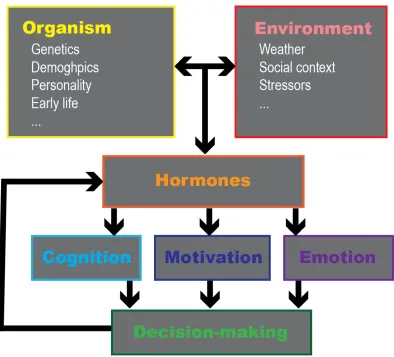
seconds to hours, making them immediate candidate biological mediators for trans-lating environmental changes into shifts in cognition, motivation, and emotion that influence decision-making.
Figure 1.1: A framework for studying hormonal influences on decision-making. The interaction of environmental factors and the organism’s inherent characteristics (e.g., genes) leads to hormonal variations that cause shifts in cognition, motivation and emotions and influence decision-making. Decisions might generate behaviors that influence the organism’s hormonal levels (either directly or through environmental changes), as implied by the feedback arrow.
Rubin, Paul H and C Monica Capra (2011). “The evolutionary psychology of eco-nomics”. In:Applied Evolutionary Psychology, pp. 7–15.
Rubinstein, Ariel (2008). “Comments on neuroeconomics”. In: Economics and Philosophy24.03, pp. 485–494.
Simonson, Itamar (1989). “Choice based on reasons: The case of attraction and compromise effects”. In:Journal of consumer research, pp. 158–174.
Statman, Meir (2013). “Mandatory retirement savings”. In:Financial Analysts Jour-nal69.3, pp. 14–18.
Thaler, Richard H (2000). “From homo economicus to homo sapiens”. In: The Journal of Economic Perspectives14.1, pp. 133–141.
Toplak, Maggie E, Richard F West, and Keith E Stanovich (2011). “The Cognitive Reflection Test as a predictor of performance on heuristics-and-biases tasks”. In: Memory & Cognition39.7, pp. 1275–1289.
Trueblood, Jennifer S et al. (2013). “Not just for consumers context effects are fundamental to decision making”. In:Psychological science24.6, pp. 901–908. Wang, Christina et al. (2004). “Measurement of total serum testosterone in adult
men: comparison of current laboratory methods versus liquid chromatography-tandem mass spectrometry”. In:The Journal of Clinical Endocrinology & Metabolism 89.2, pp. 534–543.
Wang, Joseph Tao-yi, Michael Spezio, and Colin F Camerer (2010). “Pinocchio’s pupil: using eyetracking and pupil dilation to understand truth telling and de-ception in sender-receiver games”. In: The American Economic Review 100.3, pp. 984–1007.
Welker, Michael (1995). “Disclosure Policy, Information Asymmetry, and Liquidity in Equity Markets*”. In:Contemporary accounting research11.2, pp. 801–827. Zhu, Wei Xing, Li Lu, and Therese Hesketh (2009). “China’s excess males, sex
C h a p t e r 2
EXTRAPOLATIVE BELIEFS IN PERCEPTUAL AND
ECONOMIC DECISIONS: EVIDENCE OF A COMMON
ABSTRACT
and perceptual decision domains, then (i) a common computational model should explain belief-updating (across trials) in both tasks and (ii) individual differences in the degree to which subjects rely on recent stimulus history to update beliefs should be correlated across tasks.
2.2 Methods
Subjects
Thirty-eight subjects (17 females) aged 17-29 (mean: 20.24 SD: 3.11) participated in the study. Subjects were students at Caltech or at a nearby community college and the sample size was chosen to match the exact sample size employed in previous work with the same task (Bloomfield and Hales, 2002). The California Institute of Technology and University of Southern California Institutional Review Boards approved this study, and the subjects gave informed consent.
perceptual decision task
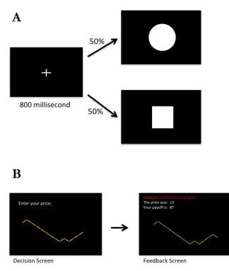
Figure 2.1: Experimental design of the task (EDT) and perceptual decision-makingtask (PDT). (A) PDT: Following a display of a fixation cross at the center of the screen (800 milliseconds), either a circle (p=.5) or a square was presented in random order over the course of 1200 trials. Subjects were incentivized to respond to each shape with a different key press as quickly and as accurately as possible. A new trial started immediately following the response, with the appearance of a new fixation cross. (B) EDT: On each of 400 trials, subjects entered the price, p, at which they would be willing to buy a stock. A price x was then randomly drawn and if x<p, the subject purchased the stock at a price of x on that trial. The stock then paid $100 if there was a positive performance surprise, and $0 otherwise.
minimize AF sequential effects (Cho et al., 2002; Gao et al., 2009).
Basic results from the economic decision-making task
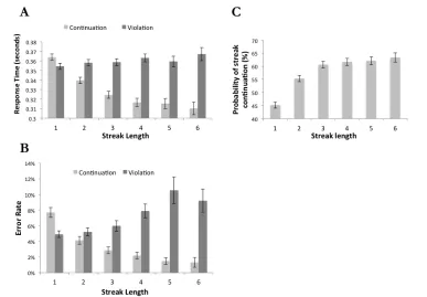
Consistent with previous research, we found substantial evidence of extrapolation based on the previous history of stimuli in the EDT (Bloomfield and Hales, 2002; As-parouhova, Hertzel, and Lemmon, 2009). Specifically, as shown in Figure 2.2c, we found that the longer the current streak of positive (negative) performance surprises, the higher the reported probability of a subsequent positive (negative) performance surprise (p< 0.001, see Table 2.6).
Figure 2.2: Basic experimental results (A) Average RT as a function of current streak length (PDT), where streak length is defined as the number of consecutive identical stimuli. Continuations are those trials where the streak continues; violations are those trials where the steak is violated. Data is shown only for correct trials (94% of the data) (B) Error rate as a function of current streak length (PDT). (C) Average reported beliefs (EDT) that the current streak would continue as a function of streak length. All error bars represent standard errors clustered at the subject level.
Structural model of decision-makingin the PDT
Drift Diffusion Model Overview
the upper threshold to a constant,a. In this model,M is the drift rate and represents the strength of incoming sensory information that a subject uses to infer the identity of the current shape. When the discriminability between the two possible stimuli is high, the drift rate is large; if instead, the two shapes are difficult to discriminate, then the incoming sensory evidence in favor of one option versus the other is low and the drift rate will be small. The variableci represents the initial point in conditioni
and can parameterize the prior bias towards selecting the correct alternative (we use the convention that the upper boundary is associated with the correct alternative). Finally,srepresents the standard deviation of mean-zero Gaussian distributed noise, which we set tos =0.1 without loss of generality, anddW is a Weiner process.4
Figure 2.3: A graphical illustration of the drift diffusion process. The bold path indicates the evolution of the relative decision value (RDV) that tracks the relative evidence in favor of the alternative associated with the upper boundary. TE denotes the time required for encoding the stimulus, TM denotes the time required for making the motor response (such that the non-decision time, T, equals to the sum of TE and TM). c denotes the initial point that captures prior bias, a denotes the upper boundary that captures the speed-accuracy trade-off, and M denotes the drift rate that represents the quality of sensory input. When the RDV reaches a boundary, the process terminates and a decision is made. Without loss of generality, the lower boundary is set to zero.
The non-decision time, denoted by T, represents the time required to encode the 4Because the noise parameters, drift rateM, and boundary separationa, are only defined up to
Figure 2.4: Average response times of correct and incorrect responses following “valid”, "neutral" and "invalid" cues.
Valid cues are repetition following two or more repetitions or alternation following two or more alternations). Invalid cues (i.e., alternation following two or more repetitions or repetition following two or more alternations) and ‘neutral’ cues are
all other trials.
Decoding prior beliefs using the DDM
Using the estimated DDM parameters, we decoded the prior probability for each subject and condition. To understand how the decoding process works, recall that the drift rate of the DDM,M, encodes the informativeness of the sensory signals in discriminating between the two shapes. At every instant within a trial, a new noisy signal is sampled where the noise is governed by the volatility of the process,s2. All else equal, whenM decreases, the signal to noise ratio decrease and a subject must rely more heavily on his prior belief. In the limit, when the drift rate goes to zero, the subject relies exclusively on his prior. In the appendix, we analytically solve for the probability of hitting the upper boundary when the drift rate goes to zero, and find that, in condition i, this prior equals ci
a. Using this analytical result, we then
collapsed the data from 16 to 8 conditions, because the identity of the current trial does not vary with the prior (e.g., trials in condition AAARand trials in condition
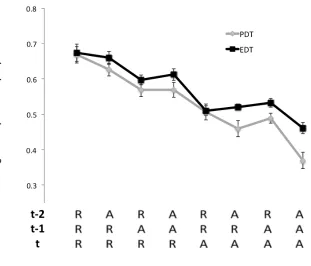
Figure 2.5: Average priors for the EDT and PDT as a function of the four most recent stimuli history. For each of the eight different conditions, the black line shows the average belief that a repetition will occur on the subsequent trial in the EDT, elicited using the BDM procedure. The gray line shows the average prior that a repetition will occur on the subsequent trial in the PDT, decoded from the initial point and boundary parameters of the DDM.
Individual differences in belief formation across tasks
Using our decoding strategy, we found significant individual differences in the extent to which priors in the PDT deviated from the rational prior of 0.5. To quantify this deviation, for each subjectu, we computed the sum of squared deviations from 0.5
and define this as the irrationality index (II):
I Iu = 1
8 8
X
i=1
(pi,u−0.5)2. (2.3)
Because subjects were explicitly told that the probability of seeing either shape was 0.5, independent of the stimulus history, a fully rational subject would exhibit an irrationality index of 0 in the PDT. Instead, we found that the average II across subjects was 1.93 (SD: 0.391), which is significantly greater than the optimal level of 0 (p < 0.001, Tobit regression left-censored at 0). If the extrapolative beliefs
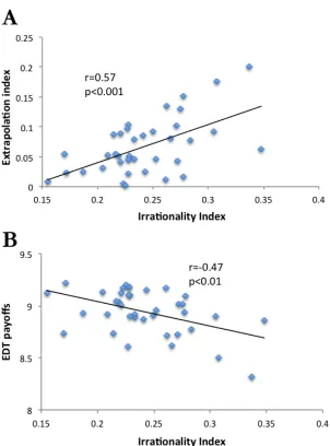
Figure 2.6: Individual differences. (A) Correlation across subjects between the extrapolation index and the irrationality index. (B) Correlation across subjects between the irrationality index and the EDT payoffs. Each point represents a single subject.
the average predictions, as indicated by the lower AIC in model (2) compared to that of model (1).
Figure 2.7: Out of sample DBM-based predictions of the average EDT beliefs. The predictions are calibrated from the PDT priors. A DBM model is estimated for each subject from the PDT. We then input the stimuli from the EDT into the DBM using the averageαacross subjects from the PDT, and generate a time series of theoretical predictions (red). The empirical average beliefs from the EDT are plotted in blue. The correlation between the two time series is.66(p< 0.001).
2.4 Discussion
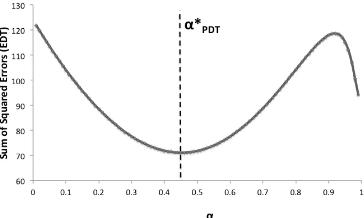
Lem-Figure 2.8: The sum of square errors of the DBM prediction for the average reported beliefs in the EDT, as a function of parameterα. The mean parameter found in the PDT,α∗, is marked by the dashed line.
Table 2.2: Individual differences in PDT predict behavior in EDT. The dependent variable is subjecti’s response on trial t of the EDT. “Average prediction” is the model prediction using the mean α from the PDT. “Individual prediction” is the model prediction using individual estimates ofαfrom the PDT. Standard errors are in parentheses and are clustered by subject.
Dependent variable: Beliefs (EDT) Average prediction 1.06∗∗∗ 0.900∗∗∗
(0.142) (0.145)
Individual prediction 0.333∗
(0.152)
Constant −0.005 −0.130
(0.073) (0.089)
Observations 15,200 15,200
AIC 791 747
R2 0.080 0.083
Note: ∗p < 0.1∗∗p < 0.05∗∗∗p< 0.01
APPENDIX
2.A Data preprocessing and order of experimental tasks
Preprocessing of reaction time data.
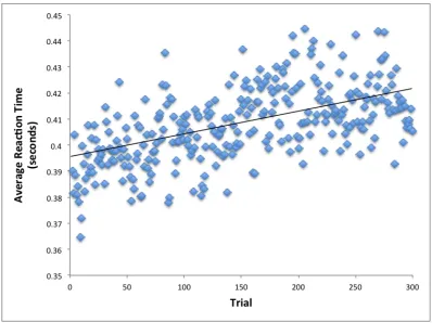
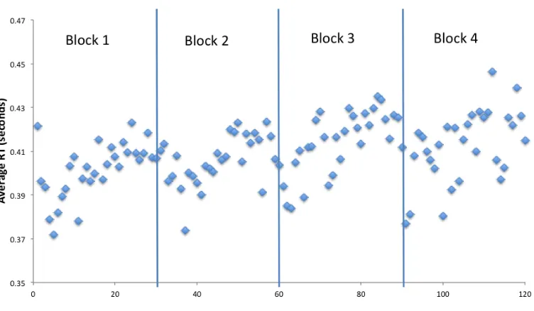
The PDT consisted of 4 blocks of 300 trials each. RTs and error rates systematically increased over the course of each block, likely due to subjects’ fatigue (See Figures 2.9 and 2.10). To control for this, we removed a linear time trend, within each block, for each subject. All results and analyses in the text use this de-trended RT data and are robust to exclusion of the de-trending step.
Figure 2.9: Average reaction times across subjects and across four blocks of trials (each data point is the average of four blocks across all subjects).
On the ordering of the tasks in the experimental session.
Figure 2.10: Average reaction times across subjects for each of the four blocks of trials (grouped by trials of 10).
Figure 2.11: Average rate of correct responses across subjects for each of the four blocks of trials (grouped by trials of 10).
against finding the extrapolation effect observed in the EDT (where subjects were not explicitly informed about the underlying random process).
2.B Robustness checks and extended statistical tests
The tables below summarize mixed model regressions estimating the effects of streak length on response times and error rates (PDT) and subjective beliefs (EDT). Table 2.3: Mixed model linear regression (subject random intercepts and slopes), PDT response times (correct)
Dependent variable: Adjusted RT (Correct trials)
Streak Length 0.002∗∗∗
(0.001)
Continuation 0.020∗∗∗
(0.004)
Streak Length x Continuation −0.015∗∗∗
(0.001)
Constant 0.394∗∗∗
(0.008)
Observations 42,476
Log likelihood 36,134.610
AIC −72,663.220
Table 2.4: Mixed model logistic regression (subject random intercepts and slopes), PDT accuracy
Dependent variable: Correct = 1
Streak Length −0.136∗∗∗
(0.028)
Continuation −1.129∗∗∗
(0.103)
Streak Length x Continuation 0.642∗∗∗
(0.042)
Constant 3.240∗∗∗
(0.100)
Observations 44,992
Log likelihood −9,327.701
AIC 18,677.400
Note: ∗p< 0.1∗∗p< 0.05∗∗∗p< 0.01
Table 2.5: Mixed model linear regression (subject random intercepts and slopes), PDT response times (incorrect)
Dependent variable: Adjusted RT (Incorrect trials)
Streak Length −0.001∗∗∗
(0.006)
Continuation −0.037∗∗∗
(0.020)
Streak Length x Continuation 0.011∗∗∗
(0.010)
Constant 0.394∗∗∗
(0.021)
Observations 2,516
Log likelihood −274.151
AIC 572.303
Table 2.6: Mixed model linear regression (subject random intercepts and slopes), EDT beliefs
Dependent variable: Beliefs (continuation) Streak Length 4.463∗∗∗
(0.586)
Constant 48.613∗∗∗
(0.669)
Observations 15,580
Log likelihood −71,203.040
AIC 142,420.100
Figure 2.12: Simulations of choosing the “correct” alternative as a function of the drift rate. For a given level of within trial noise, as the drift rate tends to zero, the probability of choosing the correct alternative converges to ca. Three different levels of ca are shown: 0.5,0.75, and 0.83.
should answer as quickly and as accurately as you can.
In each trial, the chance that you will see a circle is 12, and the chance that you will see a square is 12. Shapes on previous trials have no influence on the shape in the current trials; in other words the shape you see on the current trial is completely independent of all other shapes you’ve already seen. Before the real task starts, you will start with 5 practice trials.
Part II(instructions were given only after part I was completed)
We have studied large numbers of publicly traded companies, and constructed models of their performance patterns. Using these models, we created sequences to represent patterns of “surprises” (actual performance minus predicted performance). An upward movement indicates a “positive surprise,” which results when the firm performs better than expected, and a downward movement indicates a “negative surprise” when the firm performs worse than expected.
a stock that has 0% chance of paying you.
In each period, you will be given $100 in experimental currency to buy a share of the stock. Since the maximum price you would ever pay for a share is $100, you will always have enough cash to buy a share of this stock, since you receive a new $100 endowment each period. Your payoff in each period will depend on the three things: your willingness to pay, the actual price, and whether there was a positive or negative surprise. To illustrate your payoffs consider the two scenarios.
If you believe there will be a positive surprise for sure, and your willingness to pay is $100, and the actual price drawn is $0, and there is actually a positive surprise, then you will end the period with $100 – $0 + $100= $200. That is, you will end the period with the $100 you started with, you don’t pay any cost since the price was $0, and you earn $100 for buying the stock and having a positive earning surprise. If you believe there will be a positive surprise with 60% chance, the actual price drawn is $30, and there is a positive surprise, then your total earnings this period will be $100-$30+$100=$170.
Your final earnings will be the sum of each of your individual period earnings, di-vided by 5,000. It is important to emphasize once more: the only way to maximize your final earnings is to enter your willingness to pay equal to the probability you think there will be a positive surprise.
Usher, Marius and James L McClelland (2001). “The time course of perceptual choice: the leaky, competing accumulator model.” In:Psychological review108.3, p. 550.
Vandekerckhove, Joachim and Francis Tuerlinckx (2008). “Diffusion model analysis with MATLAB: A DMAT primer”. In:Behavior Research Methods40.1, pp. 61– 72.
Webb, Ryan (2013). “Dynamic constraints on the distribution of stochastic choice: Drift Diffusion implies Random Utility”. In:unpublished, New York University. White, Corey N and Russell A Poldrack (2014). “Decomposing bias in different
types of simple decisions.” In: Journal of Experimental Psychology: Learning, Memory, and Cognition40.2, p. 385.
Wilder, Matthew H et al. (2013). “The persistent impact of incidental experience”. In:Psychonomic bulletin & review20.6, pp. 1221–1231.
Wilder, Matthew, Matt Jones, and Michael C Mozer (2009). “Sequential effects reflect parallel learning of multiple environmental regularities”. In:Advances in neural information processing systems, pp. 2053–2061.
Woodford, Michael (2014). “Stochastic choice: An optimizing neuroeconomic model”. In:The American Economic Review104.5, pp. 495–500.
Yu, Angela J and Jonathan D Cohen (2009). “Sequential effects: superstition or ratio-nal behavior?” In:Advances in neural information processing systems, pp. 1873– 1880.
C h a p t e r 3
ABSTRACT
Figure 3.1: Experiment timeline and salivary testosterone levels. Subjects arrived at the lab at 9 am, had their hands scanned, filled an intake survey, and gave a baseline saliva sample “A” before application of either testosterone or placebo topical gel. After a four-hour loading period, subjects came back to the lab and took part in a battery of behavioral tasks. Three additional saliva samples (“B”, “C” and “D”) were collected during the experiment, all of which indicated elevated T levels in the treatment group compared to placebo. The CRT and math tasks took place between saliva sample B and C.
analyses that include these scales as control variables.
Digit ratio measurement
The ratio of second (index) finger length to fourth (ring) finger (abbreviated 2D:4D) is considered a proxy for pre-natal T exposure, and a previous study suggested that the measure correlates with CRT performance (Bosch-Domenech, Branas-Garza, and Espin, 2014). Subjects’ 2D:4D ratios were measured by two independent raters using hand scans and digital calipers (correlation between the two raters was .95). The right hand digit ratio was not calculated for one subject due to a broken finger, and therefore he was excluded from all analyses that use the right hand digit ratio as control. Correlation between the digit ratios of the left and right hands was 0.64, p=0.0001. Regression models (tables 3.6, 3.7, 3.8) are reported using the right hand measurements. All of the results hold when replacing the right hand 2D:4D by either the left hand digit ratio or the averaged digit ratio of both hands.
Cognitive reflection test (CRT)
The CRT is designed to assess a specific cognitive function: the ability to suppress an intuitive and spontaneous ("system 1") incorrect answer in favor of a reflective and deliberative ("system 2") correct answer.
The test consists of the following three questions:
1. A bat and a ball cost $1.10 in total. The bat costs $1.00 more than the ball. How much does the ball cost?
2. If it takes 5 machines 5 minutes to make 5 widgets, how long would it take 100 machines to make 100 widgets?
3. In a lake, there is a patch of lily pads. Every day, the patch doubles in size. If it takes 48 days for the patch to cover the entire lake, how long would it take for the patch to cover half of the lake?
Math task
Participants completed a math task to control for their arithmetic skills, engagement levels, attention, and motivation. They had five minutes to correctly add as many sets of five two-digit numbers as possible. Subjects could use pen and paper but were not allowed to use a calculator. The two-digit numbers in each problem were randomly drawn and presented in the following way on the computer screen (participants entered their summation of the five numbers in the blank box on the right):
Table 3.1: math task question example. 21 35 48 29 83
Once a participant submitted an answer, a new problem appeared. Participants received $1 for each correct answer and $0 for an incorrect answer.
Treatment expectancy
One previous study indicated an effect of subjects’ beliefs about the treatment they had received on behavior (Eisenegger, Naef, et al., 2010). We therefore asked subjects to indicate their expectancy about whether they had received placebo or T using a 5-point scale. There were no significant differences between the groups on this expectancy measure (see Table 3.2). Two subjects did not report their treatment expectancy and therefore were excluded from all analyses in which this measure was used as a control.
3.3 Results
We observed elevated levels of T and its metabolites (e.g., dihydrotestosterone) in the saliva measurements of the T group but not in the placebo group (Figure 3.1). There were no treatment effects on either mood, treatment expectancy, or levels of all other measured hormones, ruling out these potential indirect treatment influences on the task; see appendix for further details.
3.2c-Figure 3.2: Testosterone’s influence on CRT and math performance: behavioral results. (a) Mean CRT scores under placebo and testosterone treatments. (b) Mean arithmetic scores under placebo and testosterone treatment (c-e) proportions of answers given to each of the CRT questions separately. The left bar represents the correct, deliberate answer; the middle bar represents the incorrect intuitive answer; the right bar represent incorrect answers that are different from the intuitive one. Error bars denote 95% confidence intervals.
In non-human species, T levels typically rise during breeding season to facilitate instinctive behaviors such as mating and intra-male aggression (Edwards, 1969; Wingfield et al., 1990; Mazur, 2005; Archer, 2006; Eisenegger, Haushofer, and Fehr, 2011). In humans, the analogous effects are release of T and its precursors during competition, challenge, presence of an attractive mate, and in anticipation of sexual activity (Mazur, 2005; Archer, 2006; Eisenegger, Haushofer, and Fehr, 2011; Miller and Maner, 2009).
and profitability and longevity of high frequency traders (HFT, Coates, Gurnell, and Rustichini, 2009). HFT requires rapid processing of visuospatial information to detect temporary mispricing between markets on the scale of seconds to minutes. HFT is very likely a domain in which rapid system 1 responses are optimal. Indeed, the co-existence of systems 1 and 2 strongly suggests that system 1 responses are not always wrong or suboptimal (keeping in mind that the CRT was specifically designed to show system 1 flaws). In HFT, traders who deliberate too long will see the mispricing disappear as faster traders profitably erase it.
Table 3.2: Self-reported demographic data summary (standard errors in parentheses)
forming a compound into a derivative product of similar chemical structure—with pyridine-3-sulfonyl chloride for the estrogens (estrone (E1), estradiol (E2), and es-triol (E3)) as outlined by Xi and Spink (2008). 40 µL sodium bicarbonate (50mM, pH 10) and 40 µL pyridine-3-sulfonyl chloride (3 mg/mL in acetonitrile) were added to the dried samples, and incubated at 60oC for 10 minutes. After derivatization, the samples were diluted with 80 µL of water and injected for LC-MS/MS analysis with analytical separation performed on an Agilent Poroshell 120 EC-C8 column and ionization by atmospheric pressure chemical ionization (APCI) in the positive ionization mode.
Table 3.3: Detection levels, precision and normality tests of hormonal assays
hormone in the sample are never zero, even when they do not reach the detection threshold)
3.C Hormonal changes following treatment and manipulation check
As expected, there were significant post-treatment differences between groups with respect to all hormones influenced by T treatment, either as an upstream (androstene-dione) or downstream (5-α DHT) metabolite of T (Horton and Tait, 1966). There was also a decrease in progesterone 170H resulting from an increase in T (which is common, according to personal communication from ZRT Laboratories chief sci-entist Dr. David Zava). The changes in saliva T measures were similar in magnitude to those reported in previous studies following topical gel administration of T and progesterone (e.g. Mayo et al., 2004; Du et al., 2013).
Table 3.4: Hormone panel data measurements log(pg/mL) summary statistics (stan-dard errors in parentheses)
saliva sample (i.e., the third overall measurement; see table 3.8).
In models (B1-B4), summarized in table 3.7, we repeated the analyses of models (A1)-(A4), where the binary treatment variable was replaced by the measurements of the hormones that are affected by the treatment (T, DHT, androstenedione, and progesterone 170H).
Table 3.9: CRT score response frequencies and statistics by question
CRT, question level
We further examined the effect of T on each of the three CRT questions separately. For each question, we classified the responses as either (a) an intuitive incorrect answer, i.e., 10 cents in the “bat and the ball” question, 100 minutes in the “widgets” question, 24 in the “lily pads” question; (b) the reflective, correct answer, i.e., 5 cents in the “bat and the ball” question, 5 minutes in the “widgets” question, 47 in the “lily pads” question; or (c) another incorrect answer, i.e., different than in (a) or (b).
Dual hormone interactions
Response times
C h a p t e r 4
ABSTRACT
Players cannot commit to a particular bargaining position. In case of agreement on an uniformed player’s payoff w, the informed player gets y = π−w. If no deal is made by timeT, both players’ payoffs are zero.
The direct bargaining mechanism
By the revelation principle (Myerson, 1979; Myerson, 1984), for any Nash equi-librium in the bargaining game, there exists a payoff-equivalent equiequi-librium of a simplified game (“a direct mechanism”) in which the informed player truthfully reveals the pie size to a neutral “mediator” who determines the payoffs and the probability of a strike based on that report (Forsythe, Kennan, and Sopher, 1991). Following FKS, we assume that bargainers negotiate inscrutably over the set of direct mechanisms of the following type.
In the direct mechanism, the informed player announces the true size of the pie,πk.
The pie is then decreased by a known fraction, 1−γk, which can be interpreted as the strike probability in statek, leaving an expected pie size ofγkπk. We refer toγk
as the deal probability and 1−γkas the strike probability. The uninformed bargainer
receives xk, and the informed player gets the rest of the pie, γkπk − xk. To make
predictions regarding observed behavior, we rely on the fact that the payoffxkin the
direct mechanism is tantamount to the expected payoff of the uninformed player in state k of the bargaining game: xk = γkwk such that wk is the uninformed payoff
conditional upon a deal in statek. A mechanism therefore involves 2K parameters, {γk,xk}Kk=
1.
Individual rationality (IR)
Individual rationality requires that both players prefer to participate in the mecha-nism. Therefore, the IR requirement is that for allk
γkπk −xk ≥ 0 (4.1)
xk ≥ 0. (4.2)
Incentive compatibility (IC)
A mechanism is IC if it is optimal for the informed player to tell the truth, i.e., her expected payoff is (weakly) maximized when she announces the true size of the pie. This requires
2. In each game, an integer pie size, π ∈ {$1,2,3,4,5,6}, was drawn from a commonly known discrete uniform distribution:
Pr(πk) =
1
6 ∀π ∈ {$1,2,3,4,5,6}.
3. The informed player was told the true value ofπ for that period.
4. Each pair bargained over the uninformed player’s payoff, denoted byw. Players communicated their monetary offers, in multiples of $0.2, using mouse clicks on a graphical interface that was designed for this purpose by z-tree software (Fischbacher, 2007)5(see Figure 4.1). The offer values were between $0 and $6.
5. During the first two seconds of bargaining, both players fixed their initial offers, without seeing the offers of their partner (see Figure 4.1a).
6. Once the initial offers were set, players bargained continuously for 10 seconds using mouse clicks (see Figure 4.1b).
7. When players’ positions matched each other, visual feedback was given to both of them in the form of a vertical stripe connecting their offer lines (see Figure 1c). If none of the players changed their position for the next 1.5 seconds following the offer-match feedback, a deal was made. Thus, in order to make a deal, the latest time in which players’ bids could match wast =8.5
seconds.
8. If no deal had been made within 10 seconds of bargaining, both players’ payoffs from that period were $0.
9. After each game, both players were told their payoffs and the actual pie size (see Figure 4.1d).
Methods
We conducted eight experiment sessions, five at the Caltech SSEL and three at the UCLA CASSEL labs. There were a total of N=110 subjects (mean age: 21.3 SD: 5A video demonstration of the task is available onhttps://www.youtube.com/watch?v=
Figure 4.1: Bargaining interface. (a) initial offer screen: in the first two seconds of bargaining, players set their initial position, oblivious to the initial position of their partner. The pie size at the top left corner appears only for the informed type. (b) Players communicate their offers using mouse click on the interface. (c) When demands match, feedback in the form of a green vertical stripe appears on the screen. If no changes are made in the following 1.5 seconds, a deal is made. (d) Following the game, both players are notified regarding their payoffs and the pie size.
2.4; 47 females). The number of subjects varied slightly across sessions due to show-up differences (see Appendix 4.B for details)6. In the beginning of each session, subjects were randomly assigned to isolated computer workstations and were handed printed versions of the instructions (see Appendix 4.D). The instructions were also read aloud by the experimenter (who was the same person in all sessions). All of the participants completed a short quiz to check their understanding of the task. Subjects played 15 practice rounds in order to become familiar with the game and the interactive interface before the actual play of 120 periods. Participants’ payoffs were based on their profits in randomly chosen 15% of the periods, plus a show-up fee of $5. Each session lasted approximately 90 minutes.
6There is a negative correlation (r =−0.49) between session size and overall deal rate, which
Table 4.1: Average payoffs* and deal rates by pie size**, standard errors in paran-theses
Pie size 1 2 3 4 5 6 Mean
Informed payoff 0.37 0.95 1.56 2.23 3.07 3.87 2.01
(0.03) (0.04) (0.04) (0.03) (0.05) (0.06)
Uninformed payoff 0.63 1.05 1.44 1.77 1.93 2.13 1.49
(0.03) (0.04) (0.04) (0.03) (0.05) (0.06)
deal rate 0.42 0.48 0.54 0.69 0.73 0.81 0.61
(0.06) (0.05) (0.03) (0.02) (0.02) (0.02)
Surplus Loss 0.58 1.04 1.39 1.25 1.36 1.16 1.13
(0.06) (0.10) (0.10) (0.10) (0.10) (0.11)
Information value*** -0.11 -0.05 0.05 0.31 0.83 1.39 0.40
Figure 4.2: Deal rates and mean payoffs across pie sizes. Standard errors are calculated at the session level.
(a) deal rates by pie size
(b) Mean payoffs by pie size and subject type, periods ending in a deal. Standard errors are calculated at the session level.
modes are$2and there are local maxima at the half of the pie.
The distributions of uninformed players’ payoffs are in Figure 4.3. The mean payoffs (conditional upon a deal being reached) are in Figure 4.2B.
Result 3. The informed players’ offers increase, and the uninformed players’ de-mands decrease with time (within a trial).
Result 3 is illustrated by the plots of mean bargaining positions shown in Figure 4.4. Result 4. Most deals are made close to the deadline.
Figure 4.3: Uninformed player’s payoff relative frequencies (deal games, binned in a $0.25 resolution). The green bar locates the half of the pie in each distribution.
effect” reported in previous studies of unstructured bargaining with full information (Roth, Murnighan, and Schoumaker, 1988; Gächter and Riedl, 2005).
Comparison with focal equilibria
We now turn to testing the qualitative and quantitative predictions derived from the bargaining theory. In particular, we test the predictions of the efficient and equal-split equilibria. For convenience, we refer to the informed and uninformed players’ bargaining positions as ‘offers’ and ‘demands’, respectively.
Payoff distributions
Overall, 82% of the payoffs, conditional upon a deal being reached, match values that are halves of one of the six possible pies.8 Equal splits are the most prevalent 8In our experimental interface, players communicated their bids in integer multiples of 0.2, and
Figure 4.4: Mean bargaining position for all pie sizes (all periods pooled)
Figure 4.6: Uninformed player’s initial demands (pooled across all games, binned in a $0.25 resolution).
strikes are common (19%), even at the largest pie size of 6– in contrast to the predictions of both equilibria. It is important to note that in some interesting models, and under certain experimental conditions, strikes can occur even with complete information (e.g. Roth and Michael W Malouf, 1979; Roth, Michael WK Malouf, and Murnighan, 1981; Roth and Murnighan, 1982; Roth, 1985; Haller and Holden, 1990; Herreiner and Puppe, 2004; Gächter and Riedl, 2005; Gachter and Riedl, 2006; Embrey, Hyndman, and Riedl, 2014). If the forces operating in such models and environments also apply in our private-information settings, the strike rates could be larger than those predicted by the mechanism design approach. One factor that might account for disagreement rates that are higher than predicted is false revelations made by the informed players (i.e., offers that are too low). To assess the role of this factor, we estimated three logistic regression models with the dependent measuredeal = 1 (i.e., strike= 0), that included subject-level dummy variables (for both informed and uninformed players) and control for period.10 We estimated a model that includes the pie size alone (Model A), the final offer made by the informed player alone (B) 11, and both pie size and final offers (C). Our analysis (Table 4.2) reveals that Model B, which includes the final offers, fits the data better than Model A which includes the pie size, as implied by a lower Akaike Information Criterion (AIC) score. Furthermore, when including both the pie size
10The regression effects are robust to inclusion/exclusion of these controls.
11All bargaining positions lacked the players’ ability to commit, with the exception of (a) positions
Figure 4.7: Empirical and theoretical deal rates for informed player’s final offer matching pie halves (standard errors are clustered at the session level)
.
Figure 4.8: Strike prediction using bargaining process data, Receiver Operating Characteristic (ROC). The dashed lines represent the false and true positive rates of a random classifier.
APPENDIX
4.A Mathematical Appendix
Proof of Lemma 1
As noted in the main text (Equation 4.3) individual rationality (IR) and incentive compatibility (IC) for the informed player imply that:
γkπk −xk ≥ γjπk −xj for all j , k.
We restate Lemma 1 here:
Lemma 1. If the bargaining mechanism satisfies IR and IC:
1. deal rates are monotonically increasing in the pie sizek.
2. The uninformed player’s payoffs are monotonically increasing in the pie size. 3. The uninformed player’s payoff is identical for all states in which the deal
probability is 1.
We first show thatγk is decreasing ink (Lemma 1.1), and then rely on Lemma 1.1
for the proofs of Lemmas 1.2 and 1.3.
Proof. Considerπk andπk+1. Incentive compatibility requires γkπk−xk ≥ γk+1πk−xk+1 γk+1πk+1−xk+1 ≥ γkπk+1−xk.
These two equations imply that
(γk+1−γk)πk+1 ≥ xk+1− xk ≥ (γk+1−γk)πk (4.11)
and therefore
(γk+1−γk)(πk+1−πk) ≥ 0. (4.12)
By definition, πk+1 ≥ πk, so then γk+1 ≥ γk, and therefore the disagreement (or
strike) rate 1−γk is monotonically decreasing in the pie size.
4.5). Qualitatively, deal rates and payoff were monotonically increasing with the pie for both groups. The largest difference observed was 8 percent increase of efficiency (deal rates) in the second half compared to the first one, when the pie was $6. We further used a 2-sided t-test to compare the two halves. While for some of the pies we found statistically significant differences at the 0.05 level (in particular, deal rates were higher and informed players’ payoffs in case of a deal were lower at the Caltech pool), none of the differences survived correction for multiple hypothesis (pmax =0.24 using Bonferroni correction).
Table 4.5: Average payoffs (case of deal) and deal rates by pie size, first vs. second half of the trials
Pie size 1 2 3 4 5 6
deal rates First 60 0.38 0.47 0.49 0.63 0.72 0.76
Last 60 0.39 0.45 0.58 0.70 0.73 0.84 p-value* 0.97 0.61 0.07 0.09 0.68 0.02
Payoff, informed First 60 0.43 1.02 1.63 2.32 3.17 4.03
Last 60 0.31 0.91 1.52 2.23 3.05 3.89 p-value* 0.08 0.03 0.08 0.15 0.10 0.13
Payoff, uninformed First 60 0.60 1.04 1.41 1.74 1.88 2.00
Last 60 0.68 1.13 1.53 1.82 1.99 2.17 p-value* 0.14 0.07 0.04 0.15 0.10 0.02 *Two-sided t-tests, uncorrected for multiple comparisons.
4.C List of process features and associated marginal effects
Figure, 4.10 summarizes all of the process features used to predict bargaining outcomes. We provide further details of calculating some of the features below. Initial difference negative? A binary indicator that equals one if the initial offer of the informed player is greater than the initial uninformed player’s demand and zero otherwise.
Positions ever matched? A binary indicator that equals one if the players’ bargain-ing positions had previously matched and they later changed their minds.
4.D instructions
This is an experiment about bargaining. You will play 120 rounds of a bargaining game.
In the game, one participant (the informed player) is told the total amount of money (pie size) in each round. This amount will be $1,2,3,4,5, or 6, chosen randomly in each trial. The amount will appear on the top left corner of the screen.
The other player is not informed of the pie size.
During each round, participants bargain over the uninformed player’s payoff.
The roles are randomly selected and fixed for the duration of the experiment. Before each round, informed and uninformed players are randomly matched.
Participants negotiate by clicking on a scale from $0 to 6 (see Figure 1). Amounts on the scale represent the uninformed player’s payoff.
During the first 2 seconds, participants select their initial offers. Note that the initial location of the cursors is random. In the following 10 seconds, the partici-pants bargain, using the mouse to select payoffs for the uninformed player. Clicking the mouse on a different part of the scale moves the cursor.
A deal occurs when the cursors are in the same place for 1.5 seconds. When both cursors are in the same place on the scale, a green rectangle will appear (see Figure 2).
If a deal is made, the informed player’s payoff is equal to the pie size minus the negotiated uninformed player’s payoff. If the agreement exceeds the total amount of money, the payoff will be negative.
If no deal has been made after 10 seconds of bargaining, both participants get $0.
The game has total 120 trials.
Before the experiment begins there will be 15 training trials, to allow you to practice.
At the end of the game, you will receive payment based on randomly selected 10% of your trials.
You will receive a $5 participation fee in addition to whatever you earn from playing the game.
Quiz
Total amount is $3. Cursors were matched in $1. How much money does the informed participant get? How much does the uninformed participant get?
Total amount is $2. Cursors were matched in $4.1. How much money does the informed participant get? How much does the uninformed participant get?
One second before the end of the trial, both participants have agreed on payoff of $2 and the green rectangle appears. What is going to happen when the trial ends?
experi-Thompson, Leigh L, Jiunwen Wang, and Brian C Gunia (2010). “Negotiation”. In: Annual review of psychology61, pp. 491–515.
Tibshirani, Robert (1996). “Regression shrinkage and selection via the lasso”. In: Journal of the Royal Statistical Society. Series B (Methodological), pp. 267–288. Valley, Kathleen et al. (2002). “How communication improves efficiency in
bargain-ing games”. In:Games and Economic Behavior38.1, pp. 127–155.
Van Poucke, Dirk and Marc Buelens (2002). “Predicting the outcome of a two-party price negotiation: Contribution of reservation price, aspiration price and opening offer”. In:Journal of Economic Psychology23.1, pp. 67–76.
Varian, Hal R (2014). “Big data: New tricks for econometrics”. In:The Journal of Economic Perspectives28.2, pp. 3–27.
Wang, Joseph Tao-yi, Michael Spezio, and Colin F Camerer (2010). “Pinocchio’s pupil: using eyetracking and pupil dilation to understand truth telling and de-ception in sender-receiver games”. In: The American Economic Review 100.3, pp. 984–1007.
White, Sally Blount and Margaret A Neale (1994). “The role of negotiator aspi-rations and settlement expectancies in bargaining outcomes”. In:Organizational Behavior and Human Decision Processes57.2, pp. 303–317.
White, Sally Blount, Kathleen L Valley, et al. (1994). “Alternative models of price behavior in dyadic negotiations: Market prices, reservation prices, and negotiator aspirations”. In:Organizational Behavior and Human Decision Processes57.3, pp. 430–447.
Young, H Peyton and Mary A Burke (2001). “Competition and custom in economic contracts: a case study of Illinois agriculture”. In:American Economic Review, pp. 559–573.
C h a p t e r 5
CONCLUSION
Over the past few decades, research in the field of Behavioral Economics has led to extensive documentation of systematic biases from the "rational" benchmark in human decision-making. Many biases persist in seemingly efficient market environ-ments, and endure even when incentives are high and learning is beneficial. These findings have challenged many core assumptions underlying traditional economic models, and their impact has been far reaching.
An important catalyst of Behavioral Economics research was the development of experimental methodologies for quantifying and describing human behavior in the laboratory. In this sense, behavioral economics’ role in advancing the understanding of how humans make decisions is akin to the role that Psychophysics had in the progress of vision research. Much of what we know about vision today had emerged from extensive documentation of perceptual biases in carefully controlled laboratory settings, along with the development of metrics and experimental methodologies in the field of Psychophysics.
Behavioral Economics offers a descriptive level of analysis, which is an essen-tial step towards understanding the phenomena it studies. For the case of vision research, much of the impetus that followed required two additional levels of anal-ysis, originally suggested by David Marr (Marr and Poggio, 1976). In Marr’s framework, Psychophysics served as the “computational” level of analysis, mapping the correspondence between a visual environment and a psychological representa-tion. Psychophysics was combined with an “algorithmic” level analysis, aiming to reverse-engineer the process that generates the mapping in a formal mathematical fashion, and an “implementation” level analysis designed to test the feasibility of the algorithmic hypotheses using biological and neural data.
expres-sions, hormonal levels, and more, allow generalizing Marr’s framework to studying the mechanisms underlying economics choice in a tri-level analysis:
Computational: finding the correspondence between stimulus and actions, as traditionally studied by experimental and behavioral economists.
Algorithmic: reverse-engineering the cognitive processes that might generate the observed computational correspondence, taking into account biological aspects (e.g., computational constraints, processing speed) and the type of problems that the human brain has honed to solve over the coarse of evolution.
Implementation: testing the feasibility of the algorithmic hypothesis, using bio-logical and neural models and data.
The current dissertation demonstrates the potential contribution of this tri-level framework. The first chapter illuminates a well-documented decision bias, extrap-olative belief formation. In contrast to the traditional economic approach of deriving predictions that are based on ad-hoc axiomatic statements (Rabin, 2000), I propose a neurally plausible algorithm (Yu and Cohen, 2009), which theoretical predictions closely match the behavioral data. The two other chapters further demonstrate how biological variables (hormonal levels) and non-choice measurements (bargaining process data), that are traditionally ignored by economists, can be used for predict-ing meanpredict-ingful economic outcomes. I am hopeful that this work will set the grounds for further investigations at the algorithmic level, that will shed further light on how these “hidden” variables influence welfare loss due to inaccurate responses (e.g., incorrect CRT answers) and costly disagreements in bargaining.
BIBLIOGRAPHY
Marr, David and Tomaso Poggio (1976). “From understanding computation to un-derstanding neural circuitry”. In:
Rabin, Matthew et al. (2000).Inference by believers in the law of small numbers. Institute of Business and Economic Research.
stress, 4, 62
strike, 7, 8, 90–101, 104, 108–110, 112–118, 120–125 strike condition, 94, 98–100, 110, 121, 124
T
tables, 30, 35, 42–44
testosterone, 6, 56–69, 71–73, 79, 80, 82 treatment expectancy, 56, 64, 65, 69, 73 U
ultimatum, 57, 95, 108 W
willingness to pay, 19 working memory, 36 Z