A time series controller algorithm for feedback control

VICTORIA ~ UNIVERSITY

•

:

" z

z 0 ; 0

..

DEPARTMENT OF COMPUTER AND

MATHEMATICAL SCIENCES

A Time Series Controller Algorithm

For F eedhack Control

Venkatesan Gopalachary

88 STAT 5

May 1997

TECHNICAL REPORT

VICTORIA UNIVERSITY OF TECHNOLOGY

P 0BOX14428

MELBOURNE CITY MC

VIC 8001

AUSTRALIA

TELEPHONE (03) 9688 4492

FACSIMILE (03) 9688 4050

A

TIME SERIES CONTROLLER ALGORITHM

FOR FEEDBACK CONTROL

VENKA TESA."' GOP ALA CHARY

Department of Computer and Mathematical Sciences, Victoria University of Technology, PO Box 14428}vfCMC, Melbourne 8001, Australia

ABSTRACT

Statisticians and control engineers, often taking different perspectives, have long practised the 'art' of process control. In recent years, the focus of attention has been on bringing the statistical process control (SPC) and automatic process control (APC)

methodologies closer together. Some of the issues of automatic process control, in particular, of continuous processes, in the existence of dead time (time delay), such as stability of the closed loop, (feedback control path), are discussed in this paper. Derivations for the general formulae for making an input adjustment that would yield the smallest possible mean square error (variance) of the output controlled variable are available in the literature. However, a method to derive a time series (stochastic) feedback control algorithm for making an adjustment in the input manipulated variable that would yield minimum variance at the output is described by considering a concrete example of a the critically damped second-order dynamic system with delay (dead time). One of the main aims of this paper is to show that such a stochastic feedback control algorithm has the benefits of both integral control and dead-time compensation while providing minimum variance control.

1 INTRODUCTION

The manufacture of products of a desired quality are realised by monitoring and controlling production and by adjusting a process variable or variables in order to maintain a performance criterion in some desirable neighbourhood of a given target value, (called 'set points'). This control action is possible by an appropriatefeedback or

procedures. Various forms of feedback and feedforward control regulation schemes are

used in automatic process control (APC) for process adjustment (control action) to make

the required change in the input in order to compensate for the output deviation. An

approach to control is to fore cast the output deviation from target which would occur if no action were taken and then act so as to cancel out this deviation. If no compensatory adjustments are made by taking proper control action, the process drifts off target and

the output follows the course of the 'disturbance' (noise).

The term 'controlled process' is often used to mean a 'process state' that is

(narrowly) interpreted as stationary having iid variation about a target value. An alternative has a 'state of control' as a process state in which future behaviour can be predicted within probability limits determined by a common-cause system (Box and

Kramer [1992]).

If a state of statistical control is identified by a process generating independent and identically distributed (iid) random variables, control of such random processes by

automatic means invariably leads to an undesirable increase in process variability. So,

APC must be properly applied to obtain successful results.

APC, also referred to as 'engineering feedback control', is an approach to

minimise the (unexpected) (output) variation (due to the presence of non-random

causes), by transferring the predictable component of the output variation to the input

manipulated variable [MacGregor] (Box and Kramer [1992]). The appropriate

engineering control strategy depends upon (i) the characteristics of the stochastic (statistical) component of the process modelled by a suitable time series and (ii) the costs associated with making dynamic adjustments.

The general purpose of automatic control is to get satisfactory process operation

by adjustment of a controller (control mechanism). By using a logical method for

selecting controller adjustments and by suitable tuning, there is the potential for efficient

process operation. It is possible to formulate a control mechanism by suitably modelling

a process that is non-stationary but probabilistically predictable (Box and Jenkins [1970].

2 STOCHASTIC MODELS

A disturbance causes a process to drift off target, and so it is necessary to

of a process, can be envisaged as the result of a sequence of independent random shocks,

and represented by (linear) differential equations. Similarly, linear difference equations

represent discrete processes in which the sampling intervals are short enough to account

for the dynamic or inertial properties of a process.

The class of non-stationary stochastic time series models, called Autoregressive

Integrated Moving Average (AR.Th1A) models, are used to describe and model certain

disturbances that regularly occur in industrial processes and the process dynamics

(inertia). The models are used also to design feedforward and feedback control schemes.

3 CONTROLLERS

In automatic controllers, the input control actions (adjustments) help bring the

process into a state of control by means of discrete data obtained through measurements.

With the process data available, it is possible to control the mean square error, (sum of

the squared deviations between an output and target value), about the target by

(proportional -integral) feedback control schemes.

PID, (three-term) controllers, are continuous time controllers. It is believed that

these controllers (i) are not capable of providing (tight) control over processes in which

the effect of an adjustment is delayed until the following sample due to time taken to

deliver material from the point of adjustment to the sample point (called, the 'dead

time'), (ii) tend to perform poorly unless 'detuned' in the face of dead times in order to

take necessary action at each sampling instant (Harris, MacGregor & Wright [1982]),

and (iii) are not (ideally) suited for direct-digital (discrete) control. In certain situations, the capability of the PID controllers may be limited to produce control actions that might

be called for by a minimum variance feedback controller. Time series controllers employ

stochastic characteristics to regulate production processes. Time series controllers

provide tight control of processes with dead time and minimum variance at the same

time.

4 TIME SERIES CONTROLLERS-CHARACTERISTICS AND FEATURES

Time series controllers are used in the process industries for regulating quality

variables measured at discrete time intervals. Their 'stochastic feedback control

disturbances. AR.IMA models forecast the drifting behaviour of the disturbances and the

stochastic feedback control algorithm or equation derived from the AR.IMA models

calculates a series of adjustments that compensate for the disturbances by making an

adjustment at every sample point.

5 MINIMUM VARIANCE CONTROL

A feedback control strategy to minimise the mean square of the output deviation

(error) from target is by minimum mean square error or variance control. It is possible

that minimum variance control can be achieved in processes described by linear functions

with disturbances which are added together and treated as a single disturbance for

purposes of mathematical analysis and convenience. Though its implementation may

demand aggressive control much in excess of what is (normally) required, minimum

variance control provides a convenient bound on achievable performance against which

the performance of other controllers can be compared. Such a basis is important in the

context of deciding corrective control actions.

Time series controllers are capable of giving minimum control (error) variance

even when there are dynamics (inertia) and dead time (delay) in a process. It may be

possible to restrict sampling a process until an acceptable minimum of control error

variance can be achieved by making use of the time series controller's minimum variance

control property and to minimise monitoring and adjustment costs.

6 FEEDBACK CONTROL DIFFERENCE EQUATION

Notation

The 'stochastic feedback control (linear) difference equation' for a first-order

single-input, single-output (SISO) dynamic (process) (control) system with b units of

delay can be (approximately) represented by b

Yt(l-oB) = g(I-o)Xt-b

=

g(I-o)B xt, 0 ~ 8 <l (1)

where

X is the setting of the input manipulative variable (Linear function of et and of t+

integral over time of past errors, et),

e is the forecast error, t

z

_t is the disturbance,

Y _t is the output or controlled variable and

e =Z+Y

t t t'

g is the (steady-state) gain denoting the ratio of change in the steady-state process output

to the change in the input which caused it (Deshpande and Ash [ 1981 ]), (Shinskey

[1988]),

8 represents the (dynamics) inertial capacity of a process to recover back to its

(equilibrium) conditions after an adjustment is made to the process and due to which the

adjustments do not have an immediate effect on the process and

Bb Xt = Xt-b·

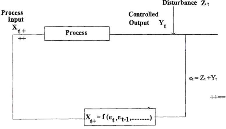
The block diagram for the feedback control model is shown in Figure 1.

Disturbance Z t Process

Input xt+

++

I

I

Controlled

Output Yt

Process

I

I

'---+)xt+

=

f (et ,et-1, ... )

-:--~

Figure 1 Block Diagram for the Feedback Control Model

et= Zt+Yt

++==

In the feedback control model shown in Figure 1, the process is regulated by

manipulating the input variable Xt+ which in tum affects the controlled output Y t· The

plus sign on the subscript of Xt+ implies that the adjustment is made during the interval

between t and t+ 1. The definite deterministic relationship existing between the process

input Xt and its output Yt described by Equation (1) does not exhibit stochastic

characteristics. Z, a non-stationary disturbance, is the output of the (linear) system,

t

For this feedback control first-order difference equation for the dynamic model

that can approximate the behaviour of a number of processes, the output change

asymptotically approaches 'g' for a unit change in the input.

7 JUSTIFICATION FOR CONSIDERING SECOND-ORDER MODELS

For feedback control (closed-loop) stability, the dynamic (inertial) parameter 8

must satisfy the condition that 0 < 8 < 1 for the discrete dynamic model of the process and the gain should be less than or equal to 1.0 (Shinskey [ 1988]).

The first-order dynamic model characterised by the linear difference equation (1)

can be written as

Yt = 8Yt-l

+

g(l-8)Xt-b • _0$8<1 (2)

The :rvt:MSE (minimum mean square error) or minimum variance control schemes

based on the first-order dynamic model and the ARTh1A (0,1,1) disturbance model

produce the minimum mean square error (M:MSE) at the output requiring excessive

control action in the following situations in which (i) the values of 8 are not fairly small;

and in (ii) as 8 becomes larger and in particular, as it approaches unity (Box and Kramer

[1992]). As 8 becomes larger, the minimum variance control exhibits large 'alternating'

character in the required adjustments to give minimum output variance (Box and Kramer

[1992]).

For larger values of

o,

the general recourse is to go in for constrained variance

control schemes. In such control schemes, reduced control action is achieved at a cost of

small increases in the mean squared error at the output by placing a constraint on the

input manipulated variable.

Processes found in practice are often complex because of their dynamic

characteristics which change with . time. Approximating such processes by first-order

dynamic models does not always seem to be satisfactory. It can be shown from the

simulation study results of the time series controller for a first-order (plus dead time)

dynamic model and the ARil\1A (0, 1, 1) model that for drifting processes, for values of 8

from O to 1, the required adjustments are of alternating character and sometimes with

that some processes may have more than one dynamic element and the exact

mathematical model relating the output and the input could be greater than the

first-order. Many complicated dynamic systems can be fairly closely approximated by

second-order systems with delay (dead time). So, it is conjectured that the dynamic system will

be better described by a second-order system that is represented by a dynamic model of

the order (2, 1), ('a discretely coincident' continuous system, Box and Jenkins [1976]).

Some commonly used identification techniques are maximum likelihood or

prediction error methods and the recursive least squares method. The recursive least

squares method and its extensions require that the value of the dead time (time delay) of

the process must be known in order to account for the delay. Palmer and Shinnar [ 1979],

though were of the view that the first-order model with dead time is sufficient for

representing some of the most commonly occurring simple processes, cautioned that

complex (process) model that helps to identify processes is (also) not (very) accurate.

They contended that there had been several claims in the process industries to

second-order models coupled with delays as sufficient for most purposes. In particular, the

second-order dynamic model (transfer function) of the form with polynomials for ro(B)

and 8(B) described by

is probably the highest order that can be justified.

It can be shown that for a given stable (transfer function) dynamic model, the

higher terms in the polynomials decrease exponentially with increasing sampling interval

(T). The transfer function, [(co₀ - co

1B)/ (1- 81B - 82B 2

)] depends on the sampling interval

(T) and also on the tuning of the process controller and therefore it can be adjusted and

the numerator can be extended further if there is a large variation in the assumed 'a priori'

dead time value.

It is possible to approximate the behaviour of high-order processes by a system

having one or two time constants and . dead time. When one or two time constants

dominate (i.e. are much larger than the other time constants in the system), all the smaller

time constants ('work together') add up to produce a lag that almost resembles (pure)

dead time. It is possible also to approximate the actual input-output mathematical model

of a high-order, complex dynamic process with a simplified model consisting of a

second-order process combined with a dead-time element. The second-order model will

reduce to the first-order model if one of the two time constants of the former model is

smaller than the other (Deshpande and Ash [ 1981 ]).

Box and Jenkins [ 1963] suggested that many dynamic models could be

adequately represented by, at most, two exponential stages with variable gains and delay

governed by parameters 81, 82, g and dead time b. Box and Jenkins [1976] mentioned

also in their monograph that complex processes with dead time (delay) can reputedly be

closely approximated by second-order systems having more than one time constant,

(usually, two). This view is shared also by MacGregor [1988]. A second-order process

with dead time is a useful model for some complex processes which are fairly common

(Shinskey [1988]).

Some methodologies were suggested by MacGregor [1988], Box and Kramer

[1992] to use statistical process control charts to monitor the performance of

closed-loop controlled systems. Such methodologies, though taking care of on-line process

control and monitoring, do not always seem to deal with stability problems of the

controlling a second-order dynamic system by a second-order dynamic model of the

form:-(3)

For stability reasons, interest is focus: ed on the 'critically damped' behaviour of

the second-order dynamic system (for which the time constants -r

1 and -r2 are real and

equal) and not on the behaviour of the system when it is either 'overdamped' or

'underdamped' for which 't

1 and -r2 may be complex.

The second-order dynamic system can then be thought of as equivalent to two

discrete first-order systems arranged in series.

The order model will be critically damped, when the roots of the

second-order model described by Equation (3) are real and equal, that is, when

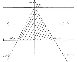
Stability is achieved when the point (81 , 82 ) lies in a triangular region defined by

the conditions 82 - 81 = 1, 01+ 82 = 1 and 82 < 1. This is shown in Figure 2.

Figure 2 Triangular region defined by the inequality conditions for achieving stability.

(4)

where ( roo - ro

1'

~ro, for mathematical convenience in dealing with a single term, being, the magnitude of the process response to a unit step change in the first period following the dead time carrying over into additional sample periods. This is possible since only

whole periods of dead time (delay) are being only considered.

Moreover, equation (4) reduces to that of Baxley's [1991] first-order dynamic

model, namely,

Yt = 8Yt-l + ro Bb+lxt·

that describes the first-order system with dead time (delay) when 82 = 0 and 81 = 8.

The steady-state gain, 'g', of such a second-order discrete dynamic model is

given by

g = (roo - ro1)/(l-81-82). (Box and Jenkins [1970])

It can be shown for a critically damped system that

ro =mo - ro1

=

PG[l - 81 - 82]

where PG represents the process gain, realised by the total effect in output caused by a

unit change in the input variable after the completion of the dynamic response (Baxley

[1991]).

Therefore, the steady-state or system gain

g

=

(roo -co1)/(1 - 81 - 82)

=

PG[l- 81- 82]/[l- 81- 82] =PG, the process gain. Baxley [1991] used PG =1/1-8 and made PG= 1.0 by setting 8 = 0, meaning that

there are no carry-over effects (inertia) and seems to have tackled the problem of

feedback control stability in a convincing manner in his simulation studies for drifting

processes. Kramer [ 1990 ], derived expressions for the disturbance and the output effect

of control actions as functions of random shocks, independent of the control scheme.

Moreover, Kramer [1990] considered approaches for reducing adjustment variability.

Since, interest here is in minimising control error standard deviation, (product variability)

at the output by using the algorithm derived in the next Section, it may be worthwhile to

consider the critically damped behaviour of the second-order dynamic system for which

the time constants are real and equal thus ensuring closed-loop stability. Furthermore, it

is shown that the steady state gain of such critically damped second-order systems is PG,

An additional term in the parameter

o

,

(02) of the second-order dynamic model

makes it possible to account for more of the process dynamics for both small and large

values of 8 and to better represent the dynamic nature of the process. The additional

term Yt-2 defines the input-output relationship in a better manner than the first-order

dynamic model.

For stability of the second-order dynamic model, the parameters 81 and 02 must

satisfy the following inequality conditions given by

0 1+82 < 1

02 - 81 < 1

-1 < 82 < 1

The roots of the characteristic equation ( l -81 B-02 B2) = 0 determine the stability

of the second-order dynamic system. When these roots are real and positive, the step

response, which is the sum of two exponential terms, approaches its asymptote g, the

steady-state gain, without crossing it. It can be seen from Figure 3, (Reproduced from

figure 10.5, page 344, Box and Jenkins [1970]), that the system has no overshoot when

the characteristic equation has real positive roots. This explains the focus on the critically

damped second-order discrete dynamic model which ensures closed-loop (feedback

control) stability.

As shown in Figures 2 and 3, the values of 81 and 82 should satisfy

-2<81<2

-1 < 82 < 1.

8 EXPRESSION FOR THE CONTROL ADJUSTMENT IN THE INPUT

VARIABLE OF A TIME SERIES CONTROLLER

An expression is derived for the feedback control adjustment required in the

input manipulated variable of a time series controller for a dynamic process with dead

time (delay). Figure 4 shows the feedback control scheme to compensate a disturbance

Zt by means of a time series controller. Baxley [1991] considered the dead time equal to

one period when deriving the feedback control equation. In this Section, the feedback

Disturbance

Zt

'\)/

Process _{Controlled Output}

x

Input t+ '\ Process to be Yt _...

/ _/

controlled

e = Zt+ Yt

Time Series t

Controller /

adjustment xt

""-Figure 4 Feedback Control Scheme to compensate disturbance

z

t

by a Time Series Controller in the existence of dynamics and dead time

From Equation (4),

(1- 81B - 82B2)Yt = ro Bb+l Xt.

-T set point

-Changes are made in the input X at times t,t-l,t-2,---, immediately after

observing the disturbances zt,zt-1,zt-2,---. Because of this, a pulsed input results and the

level of X in the interval t to t+ 1 is denoted by Xt+

For this pulsed input, assume that the dynamic model which connects the input

manipulated variable Xt+ and the controlled output Y t is

yt = L(l(B)L2(B)Bb+lxt+

where,

L 1 (B) is a polynomial in B of degree r, L1(B) is a polynomial in B of degrees and

b is the number of complete intervals of pure delay before an adjustment in the input Xt+

begins to affect the output Y

t-The non-stationary disturbance is represented by the ARil\1A (0, 1, 1) model

vzt

=(I-BB)~.

Zt measures the effect at the output of an unobserved disturbance, that is, an

uncompensated non-stationary disturbance that reaches the output before it is possible

for the compensating control action to become effective, this causes the process to

wander off target. It is defined as the deviation from the target that would occur if no

It can be shown that for a time senes controller, when the disturbance is described by the ARIMA (0, 1, 1) model and there are definite carry over (inertial) effects, the adjustment (xt) in the input manipulated variable required to make the control and forecast error variances equal, is given by

Xr+ = -{L1 (B)L3( B)/( L1(B)L4(B))}Et. where the error observed at time t,

(Box and Jenkins [ 197 6])

Et= et-b-J(b+l)

and L3(B) and L4(B) are operators in B.

The expressions for L 1 (B), L1(B), L3(B) and L4(B) can be evaluated as

L1(B) =(I- B1B - 82B2),

L1(B) = PG(l- 61 - 62)

L3(B)

=

(1-8)/(1-B) and

L4(B)

=

1

+

(1-E>)B.

The control action in terms of the adjustment x

=

x - x

1 to be made at time t is

t t+ t-+

- LI (B) L3 (B)(I - B)

xt= L1(B)L4(B) Et· (page 435, Box and Jenkins [1976]).

This 'feedback control equation defines the adjustment to be made to the process at time t which would produce the feedback control action yielding the smallest possible mean square error since it exactly compensates the predicted deviation from target' (Box

and Jenkins [1968 ]).

The above equation, on substituting the expressions for L1 (B), L1(B), L3(B) and L4(B), results in

(1-81 B-62 B2)(1-0) (S)

Xt

= -

PG(l-81-B2)(1+(1-0)B) Et·

where 0 is the moving average (operator) parameter.

The control errors which tum out to be the one-step ahead forecast errors are

measured in practice.

It is known that the error Et at the output at time t is the forecast error at lead

time b+ 1 for the Zt disturbance.

So,

For the AR.IMA (0, 1, 1) model, the weights are 'VO= 1 and 'Vl=l-0, so

Et = at ~ (I - 0) ~-1 · = (1 ~(I - 0)B) at

and further,

Since (1-0)x 100 per cent of the control error will affect the future process

behaviour as per the disturbance model, for a dead time b,

and so

et=~+ (1-0)~-b

= ~[l + (1-0)Bb]

~ =~/[

1 +( l-0)B b].

Therefore, the control adjustment equation for b periods of dead time is

_ (l-61B-62B2)(1-0) et

Xt - - X •

PG(I-61-62) (I+ (1-0) Bb)

That is,

g1vmg

_ (et-81et-1-82et-2)(1-0) ( l a )

Xt - - - - ¢ Xt-b •

PG(l-81-82)

(7)

(8)

The control adjustment action given by (8) minimises the vanance of the output

controlled variable.

Equation (8) is in conformance with the feedback control action adjustment

equation ofKramer [1990] for achieving minimum variance or mean square control when

b = 0. The control adjustment action is made up of the current deviation ( ~) and the past

adjustment action xt-b (Kramer [ 1990]). It is observed also that this is similar to the

feedback control action adjustment equation for one period of dead time derived by

Baxley [1991] on taking a value 1 for b, the dead time and when there are no carry-over

effects for a time series controller. On comparison with the equation of Baxley [1991], it

is found that the first term in Equation 8 gives the integral action and the second term,

Some simulation results of Equation 8 obtained when b = 1, given below, match closely with that ofBaxley's [1991] values for the time series controller.

Comparison of Time Series Controller Performance with One Dead time Period

---theta SE (Equation 8) SE (Baxley)

0.25 1.260 1.250

0.50 1.112 1.118

0.75 1.010 1.031

9 BENEFITS OF THE INTEGR.\.L AND DEAD-TIME COMPENSATION

TERMS IN EQUATION (8)

It has been pointed out that Equation (8) contains integral action. The control obtained through the first term in Equation (8) is the discrete analog of 'integral control',

a form of adjustment employed in engineering or automatic process control. So, a

minimum variance controller built on this algorithm will be able to maintain the desired

output variable at or near a given set point (Palmor and Shinnor [ 1979]), thereby fulfilling some of the criteria specified as the requirements of a sampled-data (discrete)

controller algorithm by Palmor and Shinnar [ 1979] in their paper.

The controller algorithm, Equation (8) meets with some of the requirements of a

(discrete) sampled-data digital controller algorithm such as

(i) It is able to maintain the desired output variable at a given set point,

(ii) The algorithm leads to stable overall control and converge fast on

the desired steady state, thus ensuring asymptotic stability and provides

satisfactory performance for different types of disturbances that could

arise,

(iii) A time series (integral) controller can be designed on the basis of

Equation (8) with a minimum of information with respect to the nature of

the inputs and the structure of the system.

(iv) Such an (integral) controller will be reasonably insensitive to changes in

system limits and will be stable and perform well over a reasonable

The integrating control action is successful in eliminating 'offset' (deviation

obtained with proportional control) at the expense of reduced speed of response and

increasing the period of the feedback control loop with its phase lag. When integral time

is too long, the feedback loop is overdamped, leading to unstable conditions. Overshoot

can be avoided by setting the integral time higher than that required for (load) regulation

and can also be minimzed by limiting the rate of set-point changes (Shinskey [1988]).

During a step change of the input process variable, the closed-loop output is

serially independent when pure one-step minimum mean square control is used which is

often the practice in process control operations.

A process variable that has a uniform 'cycle' and sustained oscillations does not

threaten the stability of the feedback control system. Under integral control, the

(feedback) closed-loop oscillates with uniform amplitude. The feedback loop tends to

oscillate at the period where the system gain is unity, the integral (also known as reset)

time, that is, the time constant (I) of the controller, then, affects only the period of

oscillation which increases with damping for a controller with integral action in a

dead-time loop. It can be shown that the 'integral time' (Iu) for zero damping (which requires a

loop gain of 1.0), is 0.64PG Td where PG is the process gain and Td, the dead time

(Shinskey [1988]). A process with a dead time of 1 minute would cycle with a period of

4 minutes under integral control with oscillations sustained by an integral time constant

of about 0.64PG minutes. Control engineers endeavour constantly to have this integral

time as nearly equal to the process dead time as possible so that the process variable can

take the same path as the dead time. It is possible to achieve damping by reducing the

closed-loop (feedback) gain and by increasing the integral time as will be shown next.

The integral action term in the control adjustment equation (8), determines the

damping of the feedback control loop. The period and the integral time required for

damping are established by the process characteristics. Minimizing the integral error

ensures damping of the feedback control loop. The minimum integral (absolute) error,

(IAE), for (integral) control of dead time is achieved by setting the integral time constant

of the feedback control loop, I

=

l.6PGTd, where Td is the time delay (dead time)

(Shinskey [1988]). Under integral (floating) control, the feedback control loop tends to

oscillate with uniform amplitude and at the period where, the (pure) steady-state gain is

changes to about half of the original period. Increases in the (integral) time constant

contribute more (phase) lag to the feedback control loop and extends the period of

oscillation of the feedback control loop. There must be a rise in integral time constant so

that the controller can then contribute less (phase) lag.

Palmor and Shinnar [ 1979] observed that 'the Smith predictor is a direct result of

minimal variance strategy and that minimal variance control for processes having dead

times includes this type of dead-time compensation'. At this stage, an intuitive

conjecture, using this principle, is made that the inclusion of the dead-time compensation

term of either the Smith predictor type and/or the Dahlin's (on-line) tuning parameter,

(whose values range from 0 to 1 ), in a feedback control algorithm will also result in a

minimum variance strategy for processes with dead time. This draws on the comparison

made by Harris, MacGregor and Wright [1982] to the minimum variance controller they

derived for the process with dead time (for which the number of whole periods of delay

was equal to 2) and the Dahlin controller given in their paper. The authors showed that

the two controllers were identical upon setting the value of Dahlin's parameter, (the

discrete time constant of the closed-loop process), equal toe, the Il\.1A parameter in the

stochastic disturbance model. They reconciled the different approaches by noting that the

'Il\.1A parameter e provides information about the magnitude of the closed-loop time

constant'. Equation (8) is identical to Baxley's [1991] algorithm and includes both

integral action and dead-time compensation terms and the Il\.1A parameter 0, (whose

values range from 0 to 1 ), is set to take care of the drift (r

=

1- 0) as well as Dahlin's

parameter to compensate for the dead time. So, it follows that the variance of the output

product variable achieved by using Equation (8) with integral action and dead-time

compensation terms is a minimum. The dead-time compensation term (seemingly)

removes the delay from stabiHty considerations and definitely provides a stabilising

effect on the feedback control system. These principles are used for designing

(formulating) the discrete (sampled data) time series (integral) controller. Such a

controller will maintain the mean of the process quality variable at or near target and will

allow for a (rapid) response to process disturbances without much overcompensation or

overcorrection.

The performance of the computer-controlled algorithm depends not only on the

control engineering literature that although a second-order (conventional) control system

is stable for all values of the (controller) gain, it is likely that computer control of the

same system can give unstable response for some specific combinations of the gain and

the sampling period. This is one of the main reasons to consider the critically damped

behaviour of the second-order model.

10 CONCLUSION

In this paper, a brief discussion of minimum variance control and time series

controllers has been provided. A general feedback control equation has been derived and

a statistical control algorithm developed for the critically damped second-order dynamic

system. The discrete stochastic feedback (integral) controller can be used to reduce the

control error sigma (product variability) at the output. The justification for considering a

second-order dynamic model and its critically damped behaviour have also been

REFERENCES

(1) Baxley, Robert V. (1991). A Simulation Study Of Statistical Process Control

Algorithms For Drifting Processes, SPC in Manufacturing, Marcel Dekker, Inc.,

New York and Basel.

(2) Box, G.E.P and Jenkins, G.M. (1963). Further Contributions To Adaptive

Control: Simultaneous Estimation Of Dynamics: Non-Zero Costs, Statistics in

Physical Sciences I, 943-974.

(3) Box, G.E.P and Jenkins, G.M. (1976). Time Series Analysis: Forecasting and

Control. Holden-Day: San Francisco.

(4) Box, G.E.P and Kramer, T. (1990). Statistical Process Control and Automatic

Process Control - A Discussion, Technical Report No. 41 of the Centre for

Quality and Productivity Improvement, University of Wisconsin, U.S.A.

(5) Box, G and Kramer, T., (1992). Statistical Process Monitoring and Feedback

Adjustment--ADiscussion, Technometrics, August 1992, Volume 34, No. 3,

251-267.

(6) Deshpande, P.B. and Ash, R.H., (1981). Elements of Computer Process Control

with Advanced Control Applications, Instrument Society of America, North

Carolina, U.S.A.

(7) Harris, T.J., MacGregor, J.F. and Wrignt J.D., (1982). An Overview ofDiscrete

Stochastic Controllers: Generalized PID Algorithms with Dead-Time

Compensation, Can. J. Chem. Eng. 60, 425-432.

(8) Kramer, T.,(1990). Process Control from an Economic Point of View-Industrial

Process control, Technical Report No. 42 of the Centre for Quality and Productivity Improvement, University ofWisconsin, U.S.A.

(9) Kramer, T., (1990). Process Control from an Economic Point of View-Dynamic

Adjustment and Quadratic Costs, Technical Report No. 44 of the Centre for Quality and Productivity Improvement, University ofWisconsin, U.S.A.

(10) MacGregor, J.F., (1987). Interfaces Between Process Control and On-line

(11) MacGregor, J.F., (1988). On-line Statistical Process Control, Chemical

Engineering Progress, 84, 21-31.

(12) Palmer Z.J. and Shinnar R., Design of Sampled Data Controllers, (1979).

Industrial and Engineering Chemistry Process Design Development, Vol.18,

No. 1,8-30.

(13) Shinskey F.G., (1988). Process Control Systems, McGraw Hill Company, New

FI<i~

.

.

3

Attachment I

c

i

0.

8.,

Complex

- I

Out -2 -1 0

')

8,

•

I

•

•

•

• •

•

I

•

•

•

I

In

I

Step responses of coincident, discrete and continuous second-order system

s

having characteristic equations with real roots (Curve R) and comple

x