High-Performance Cloud Computing: VCL Case Study.

(1)

(Under the direction of Dr. Mladen Vouk.)

High performance computing used to be domain of specialties and of the relatively few. Today, as internet has become pervasive and large amounts of data are pouring in, extensive analyses of the data and simulations are gaining more importance in decision making. This fuels use of high-performance computing (HPC), more recently high-performance data (HPD) analytics in everyday workflows. For example, advanced internet searches invariably involve loosely coupled high-performance computing, large scale business analytics also requires high-performance facilities. Security analytics and large-scale scientific analytics are hard to imagine anymore without involving an HPC/HPD platform. Properly constructed clouds should be able to offer the needed services on demand.

(2)

(3)

(4)

by

Nikhil Vivek Talpallikar

A thesis submitted to the Graduate Faculty of North Carolina State University

in partial fulfillment of the requirements for the degree of

Master of Science

Computer Science

Raleigh, North Carolina 2012

APPROVED BY:

_______________________________ ______________________________

Dr. Vincent Freeh Dr. Rudra Dutta

________________________________ Dr. Mladen Vouk

(5)

DEDICATION

(6)

BIOGRAPHY

(7)

ACKNOWLEDGMENTS

I would like to express my sincere gratitude towards Dr. Mladen Vouk for providing me the help and guidance not just through the course of my thesis but throughout the course of my graduate program at North Carolina State University. I would like to thank Dr. Rudra Dutta and Dr. Vincent Freeh for serving on my thesis committee.

I am highly obliged to Dr. Gary Howell for clearing my doubts regarding the intricacies of Henry2 cluster. I would like to take this opportunity to thank David Fiala and Yongpeng Zhang for helping me while working on the ARC cluster.

(8)

LIST OF TABLES

Table 1: CPU Configuration 1: A typical node in VCL-GP cluster ... 29

Table 2: CPU Configuration 2: A node in the ARC cluster ... 37

Table 3: Ping Pong Min/Avg/Max bandwidth and latency (ARC cluster) ... 43

Table 4: Configuration of a GPGPU card in the ARC cluster ... 45

Table 5: Configuration of Tesla C2050 GPU card (used in the experiments) ... 46

Table 6: Compilers and Math Libraries on Henry2 ... 56

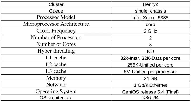
Table 7: CPU Configuration 3: A node in Henry2 cluster... 59

Table 13: Ping Pong Min/Avg/Max bandwidth and latency (Henry2 cluster) ... 70

Table 14: Processor configurations ... 72

Table 15: Minimum, Average and Maximum latency and bandwidth reported by Ping Pong test at different times (T1, T2  T1+2 days and T3 T2 + 2 hours, T4  T3 + a week) VCL-GP cluster, 4 node, 4 core test ... 80

(11)

LIST OF FIGURES

Figure 1: VCL-HPC (Henry2 cluster)... 12

Figure 2: Arc Cluster ... 18

Figure 3: HPC in VCL (VCL-GP) ... 21

Figure 4: HPL results for varying blocksize on a single VCL-GP node (1 core) ... 30

Figure 5: Maximum HPL performance for varying matrix size (N) (blocksize (NB) at which max performance was observed is noted). (Test: 4 nodes, 4 cores). Measurements were taken at different times (T1, T2  T1+2 days and T3 T2 + 2 hours) ... 31

Figure 6: HPL performance with varying block size (NB), (Test: 4 nodes, 4 cores, T2  T1+2 days and T3 T2 + 2 hours) ... 32

Figure 7: Ping-Pong network (MPI) latency, (Test: 8 Byte message, 4 nodes, 4 cores, T1, T2  T1+2 days and T3 T2 + 2 hours, T4  T3 + a week) ... 34

Figure 8: Ping-Pong network (MPI) bandwidth, (Test: 2MB messages, 4 nodes, 4 cores, T1, T2  T1+2 days and T3 T2 + 2 hours, T4  T3 + a week) ... 34

Figure 9: CPU utilization of a VCL node in the cluster, (Test: 4 nodes, 4 cores). Relative time on the x-axis is in seconds. ... 35

Figure 10: CPU utilization, single node test (1 core)... 36

Figure 11: HPL Performance, 1 node (16 cores) ... 38

Figure 12: HPL Performance, 8 node (128 cores) ... 39

Figure 13: Effect of grid mappings, 8 node (128 cores), Matrix size=1000 ... 40

Figure 16: Ping pong latency, 8 node (128 cores, 8 Byte message and 2 MB message)... 42

Figure 17: Bandwidth Test, 8 node (128 cores, 2MB message) ... 42

Figure 18: ARC cluster Peak Performance, 32 nodes (512 cores) ... 44

Figure 19: ARC cluster Peak Performance change with increase in number of cores ... 44

Figure 20: HPL performance on ARC cluster single node CPU+GPU (1 node, 1 core, 1GPU-448 cores) ... 46

(12)

Figure 22: Effect of blocksize and matrix size, 8 node (8 cores + 8 GPU) ... 48

Figure 23: Effect of number of processes on HPL performance at time T1 ... 50

Figure 24: Effect of number of processes on HPL performance at time T2 ... 50

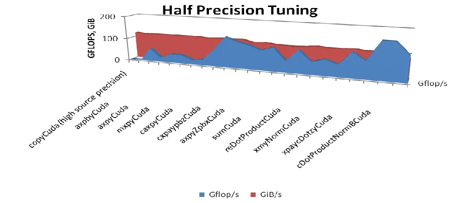
Figure 25: Tuning Half Precision floating-point operations ... 52

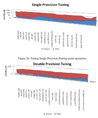
Figure 26: Tuning Single Precision floating-point operations ... 53

Figure 27: Tuning Double Precision floating-point operations ... 53

Figure 28: Performance of Dslash operations ... 54

Figure 29: Performance of Invert operations ... 55

Figure 30: Performance comparison of benchmarks on single GPU ... 56

Figure 31: HPL performance on single node, (1 node, 8 cores, CPU configuration 4) ... 62

Figure 32: HPL performance on single node, (1 node, 8 cores, CPU configuration 5) ... 63

Figure 33: HPL performance characteristics Intel compiler/Intel MKL/1G interconnect (4 node, 8 cores, CPU configuration 6) ... 64

Figure 34: HPL performance characteristics Intel compiler/Intel MKL/IB interconnect (4 node, 8 cores, CPU configuration 5) ... 65

Figure 35: HPL performance characteristics Intel compiler/GotoBLAS2 math library/1G interconnect (4 node, 8 cores, CPU configuration 6, P=2. Q=3) ... 65

Figure 36: HPL performance characteristics GNU compiler/Intel MKL/1G interconnect (4 node, 8 cores, CPU configuration 7) ... 66

Figure 37: HPL performance characteristics GNU compiler/GotoBLAS2 math library/1G interconnect (4 node, 8*4 cores, P=2, Q=3, OMP_NUM_THREADS=4, CPU configuration 8) ... 66

Figure 38: Comparison of different compilers and MKL libraries ... 67

Figure 39: Ping Pong Latency, 8 Byte message ... 68

Figure 40: Ping Pong Latency, 2 MB message ... 68

Figure 41: Ping Pong Bandwidth for 1G and InfiniBand interconnects (2MB message) ... 69

Figure 42: Ping Pong minimum bandwidth achieved for 1G and InfiniBand interconnects and the corresponding HPL performance ... 69

(13)

Figure 44: Performance for ARC cluster (4 nodes, 64 cores, OMP_NUM_THREADS=16,

CPU configuration 2) ... 71

Figure 45: Empty loop timer ... 73

Figure 46: Flops results for VCL-GP cluster node (configuration 1) ... 74

Figure 47: Flops results for Henry2 cluster node (configuration 2) ... 74

Figure 51: Max Ping Pong latency for 8 Byte message and the corresponding HPL performance (4 node, 4 core, T1, T2  T1+2 days and T3 T2 + 2 hours, T4  T3 + a week, VCL-GP cluster) ... 78

Figure 52: Max Ping Pong latency for 2 MB message and the corresponding HPL performance (4 node, 4 core, T1, T2  T1+2 days and T3 T2 + 2 hours, T4  T3 + a week, VCL-GP cluster) ... 78

Figure 53: Min Ping Pong bandwidth achieved for 2 MB message and the corresponding HPL performance (4 node, 4 core, T1, T2  T1+2 days and T3 T2 + 2 hours, T4  T3 + a week, VCL-GP cluster) ... 79

Figure 54: High Level VCL gateway provisioning architecture ... 83

Figure 55: ssh redirection setup ... 85

Figure 56: How scp works [19] ... 86

Figure 57: Web-server design ... 89

Figure 58: Web server snapshot ... 90

Figure 59: ssh agent-forwarding ... 94

Figure 60: Rocks Cluster architecture in VCL ... 99

(14)

Chapter 1 Introduction

Thirst for processing power is growing. It is driven by decision making needs, large amounts of data, analytics, simulations, and entertainment – in the research domain some examples are bio-informatics, life sciences, electronics (magnetic and electric field simulations), finance (computations for market simulation), fluid dynamics, data mining, analytics, databases, computer vision and graphics, medical imaging, quantum physics/dynamics, weather forecast simulations, geographical modeling of land and oceans, security, and similar. High-performance computing (HPC) is going mainstream – even though many do not realize that. After all, most of the high-power searches are running on platforms and on the numbers of processors that few years ago would have been considered supercomputing facilities [44]. In the last few years, one of the innovations in that domain has been the move of general purpose graphical processing units (GPGPU) into more general computing space and use of their high compute power capability to solve computational problems that exhibit high data parallelism [74,75]. GPUs come in many forms and shapes, but in most cases as add-on PCI (Peripheral Component Interconnect) cards. Traditional HPC, range from Linux clusters interconnected by high performance communication channels, to genuine, specially built supercomputers such as Cray machines [95], IBM BlueGene [93] and similar. Today, commodity hardware using just CPUs features prominently on the Top 500 list [44]. In fact, technology advances in microprocessors (e.g., multicore chips, GPU cards), network interconnects and memory technologies have brought the cost of building a high performance computer down to acceptable levels. Still, the cost of HPC does not really allow most individual users, or even companies, to have that option on their desktops or in the organization, unless those resources are shared with others.

(15)

environments are flexible in terms of new resource additions and on demand utilization. Cloud computing provides for an abstraction which is more flexible option than the traditional in-house HPC clusters. Cloud computing seems almost ideal for provisioning services that range from desktops all the way to sub-clouds and full scale HPC facilities. On the other hand there are questions related to the ability of clouds to provide adequate HPC facilities [27,30,31,32,36,37,35,43,45,47]. Most of these arguments are based on the Amazon HPC services [42]. A few arguments equate virtualization with cloud computing [34] which, of course is not true, and as a result may have an incomplete view of what a properly constructed cloud can actually do when the model includes so called hybrid computing option[42,76, 79, 50].

What is out there?

HPC in cloud is a long and interesting debate [77, 78, 79] and research area. The Amazon EC2 [1] has extended its IaaS (Infrastructure as a Service) to provision HPC and GPGPU clusters since July 2010 [32, 42], and NC State’s VCL cloud has been delivering HPC as a service since 2004 [82]. The Nimbus Project at University of Chicago and Indiana University is a similar service [83], and Beowulf clusters [84] running flavors of unix (Linux) also can provide cloud-like infrastructure for parallel computations.

(16)

Yan Zhai et al. in [27] evaluated the Amazon EC2 HPC resources in terms of overall performance, scalability, cost-effectiveness, and stability. They show that HPC in a public cloud, such as EC2, may not perform better than a dedicated in-house cluster. The main reason tends to be the communication channels (or node interconnects). EC2 uses 10Gbps Ethernet for that, while the in-house cluster may use a 40 Gbps QDR InfiniBand network. Of course, in house clusters with less communication bandwidth may not do so well. Research [27] shows that as the number of processes in a job increases the performance of EC2 cluster degrades. This is because the communication overhead increases as the number of processes increases. Also, the specialized QDR IB in-house network has less latency than the 10Gbps Ethernet on Amazon EC2 cluster [27]. There were also some performance stability issues with Amazon EC2 HPC clusters. Where Amazon EC2 appears to win, is in cost effectiveness. The average utilization of the cloud resources is higher as compared to the in-house cluster.

(17)

The following provides an overview of a non-comprehensive but reasonably representative sample of commercial on-demand HPC offerings in the cloud.

Amazon Web Services (Elastic Cloud 2)

“Amazon Web Services (AWS) [1, 42] provides affordable, flexible and on-demand compute nodes for compute intensive applications. There is flexibility to add new nodes as well as remove some nodes. HPC nodes are grouped as special high end machines which are provisioned on demand from the HPC Placement group. The nodes use 10Gbps Ethernet interconnect for MPI traffic. The AWS HPC site [1] states that “By leveraging the advanced networking and high computational capabilities of Amazon EC2 Cluster instances, customers can provision clusters that can give them supercomputing class performance without the need to build and operate their own HPC facility. For example, a 1064 instance (17024 cores) cluster of cc2.8xlarge instances was able to achieve 240.09 TeraFLOPS for the High Performance Linpack benchmark, placing the cluster at #42 in the November 2011 Top500 list”[1].

“Amazon EC2 also has a system built for provisioning GPGPU clusters. EC2 provides high bandwidth, low latency networking, and very high compute capabilities via their Cluster Compute or Cluster GPGPU instances. EC2 provides for flexible Placement Groups where each Placement Group is a tightly coupled resource cluster and offers 10Gbps full bisection network bandwidth [1]. Each GPGPU cluster can be a part of one Placement Group or multiple placement groups depending on how massively parallel the jobs are. EC2 GPGPU provisioning provides for max 2 GPU units per node. The configuration is as follows : “Cluster GPU Quadruple Extra Large 22 GB memory, 33.5 EC2 Compute Units, 2 x NVIDIA Tesla “Fermi” M2050 GPUs, 1690 GB of local instance storage, 64-bit platform, 10 Gigabit Ethernet”[1].

(18)

to performance an 880 instance (7040 cores) cluster of cc1.4xlarge instances was able to achieve 41.82 TeraFLOPS”[1]. More information can be found at [1, 42].

Nimbix

“Nimbix [7] delivers a scalable environment that extends the processing capabilities of existing high performance computing infrastructures using FPGA's and GPU's. Their computing infrastructure delivers accelerated hardware and applications that process data faster and more efficiently for industry specific tasks. Across multiple application domains, scientists and researchers are challenged by data processing requirements. Nimbix enables an easy to use service to accelerate high performance computing applications.” [7] The Nimbix site [7] quotes “NACC offers on-demand processing for HPC applications using state of the art computing infrastructure. After setting up a Nimbix account here on the portal, you may launch secure high performance computing jobs using any of a number of common HPC applications. No need to provision cloud instances or manage systems. Simply upload data, select application and submit your job. You pay only for actual processing time.” [7] This indicates that Nimbix offers pre-built common applications that run in HPC environments. The user has no control over the algorithm or code that the application is running. Nimbix offers to schedule common HPC jobs but on user provided data. This service is not a flexible service. The jobs might be running on in-house HPC clusters and there is no concept of an on demand service in this case.

PEER 1 Hosting

(19)

Hoopoe

Hoopoe [9] web services provide for GPU computer power. “A front end web service interface is used to communicate with the world and perform the various operations available by Hoopoe. Applications submit tasks, monitor activities, gather statistics, etc via the web interface. Users are not granted direct access to cluster machines, but the web service front end provides all necessary tools and features to communicate with it, perform computations, read results etc. Hoopoe's GPU cluster is composed of 10's of GPU devices, delivering more than 50 TFLOPS of peak performance. As far as internal communications is concerned, the cluster is capable of delivering over 40 Gb/s using fast InfiniBand interconnect between the nodes” [9]. Again, this model is less flexible since the user has limited access to the actual cluster.

There are various other small start-ups emerging in this domain [52, 53]. Most of the new comers are trying to copy the Amazon EC2 architecture with some smaller differences. Following are some of the open source cloud computing environments

Eucalyptus

(20)

OpenStack

OpenStack [81] is another IaaS style cloud computing platform initially developed by RackSpace [87] and NASA [88]. “It is an open source implementation, designed to provision and manage large networks of virtual machines, creating a redundant and scalable cloud computing platform. It gives you the software, control panels, and APIs required to orchestrate a cloud, including running instances, managing networks, and controlling access through users and projects [81]”. OpenStack Compute can work with different hardware platforms as well as different hypervisors available in the market. More than 150 companies have joined this project and new cloud computing startups are moving towards the OpenStack solutions, to implement their cloud computing services.

VCL (Virtual Computing Lab)

“VCL [86] is a cloud infrastructure developed and deployed in production at NCSU.” [82] “VCL is an open-source system used to dynamically provision and broker remote access to a dedicated compute environment for an end-user. The provisioned computers are typically housed in a data center (in the case of NCSU in five data centers) and may be physical blade servers, traditional rack mounted servers, or virtual machines. VCL can also broker access to standalone machines such as lab computers on a university campus [86]”. “Resource reservations are through a web interface. VCL can provision undifferentiated bare-metal or virtual machines where user is free to install any software they want and work on it for the time allocated. It can also provide blade servers running high end software (i.e. a CAD, GIS, statistical package or an Enterprise level application) and a cluster of interconnected physical (bare metal) compute nodes” [86]. VCL also has an API that can be used to automate the provisioning. Cost efficiency of VCL and of VCL-HPC is discussed in [91].

Goal of the thesis:

(21)

nodes use Rocks (Rocks is shipped with preinstalled Torque resource manager and Maui scheduler), and in the customized cluster we used Torque resource manager [68] with Maui scheduler [69] to provide VCL resources as compute nodes to the user. An aggregated cluster with certain number of preconfigured nodes can also be provisioned to the user so that the user is free to install customized resource manager and a scheduler to execute their tests in an environment that suits them. Since MPI, OpenMP and GPGPU programming using CUDA is a SIMD (Single Instruction Multiple Data) approach, users and programmers use these libraries to write applications that take advantage of data parallelism. Such applications are tightly coupled. This work explores how the performance of such real time compute intensive applications, varies when executed on different clusters. This thesis details the performance characteristics of HPL (High Performance Linpack) and Ping-Pong (network latency and bandwidth) benchmarks when run on different clusters mentioned above. Further, we discuss new methods of accessing these in-house (VCL-HPC and GPGPU) clusters. We discuss the design and implementation of a gateway server which provides an abstraction in VCL through which these in-house clusters can be accessed via VCL. We discuss the advantages and use cases of this abstraction which will enable efficient and secure implementation of HPC in future cloud infrastructures. We discuss integration of VCL and BlueGene/P as the future of HPC in cloud and explore the possibility of constructing a multi-GPU environment in a network.

Thesis Overview

In VCL we distinguish general purpose resources (VCL-GP) and high performance resources (VCL-HPC). Users can construct clusters in VCL and can access HPC facilities in the following ways.

 Existing clusters in VCL

o Preconfigured HPC facilities (VCL-HPC)

(22)

architecture of VCL-HPC in chapter 2. Chapter 3 discusses the performance characteristics of the VCL-HPC (Henry2) cluster.

o Requesting individual reservations

Users can request individual reservation for separate machines and construct a cluster using any cluster software of their choice. Depending on the privileges users may not have control over the topology or the quality of machines provisioned. Chapter 2 details the steps to construct an individual cluster using Torque resource manager and a Maui scheduler. Performance analysis of this constructed cluster is discussed in chapter 3. Use of Rocks software to construct a cluster over these individual resources is explored in chapter 4.

o Using VCL cluster reservation function

VCL provides for requesting aggregated resources with certain preconfigured properties as a cluster. The cluster then needs additional software for management purposes. We have not discussed this topic in the thesis.

 Extra clusters

HPC resources can be requested from external clusters like the NCSU ARC cluster which is not a part of the VCL subsystem. We discuss the topology and architecture of the ARC cluster in chapter 2. Chapter 3 discusses the performance characteristics of the ARC cluster. Access to this preconfigured high performance cluster in VCL is enabled by a gateway (redirection) server. The gateway server is discussed in chapter 4.

 Future Hybrid HPC/HPD facilities

o While gateway access to external HPC facilities is very useful, it will be really advantageous to have a much finer granularity control over external high performance computing resources (such as individual nodes and cores).

o Multi-GPU in a network

(23)

multi-GPU abstraction in a network and ways to access those facilities in VCL. This is discussed in chapter 5.

o VCL integration with BlueGene/P

We discuss the possibility of VCL communicating with the BlueGene/P resource manager. In the future, VCL would be able to provision clusters running on the BG/P architecture. The design for enabling this service is discussed in chapter 5.

(24)

Chapter 2 NCSU HPC Resources

There are four types of HPC resources available to NCSU researchers: 1) centrally managed VCL affiliated resources, 2) specialized HPC resources open to NCSU community (such as ARC GPGPU cluster), 3) private (research specific) HPC facilities and clusters, and 4) external resources (e.g., ORNL supercomputers). In this thesis, we limit our interest to HPC-VCL, ARC and general purpose VCL facilities that allow on-demand construction of fixed size or dynamic clusters.

We now describe the VCL-HPC architecture (pre-configured, and available to users for batch HPC processing), the architecture of the ARC GPGPU cluster, and the architecture of VCL on-demand clusters. One thing to note about configured VCL-HPC and other pre-configured NCSU HPC facilities and clusters is that the external access to those facilities (from public IP numbers) is channeled through login node(s), while the computational resources are shielded from the outside and reside on a private network. In general such resources have a tightly coupled (low latency, high inter-node communication intensity) interconnect topology and access to a large amount of either directly attached or network attached storage. On the other hand, on-demand clusters may have a more loosely coupled topology and when used as HPC framework, may be suitable only for applications that required low intensity inter-node communications.

2.1 VCL-HPC

(25)

out of VCL-HPC. If there is a surfeit of resources in VCL-GP (e.g., during holidays), those resources are shifted to VCL-HPC. VCL-HPC generates about 13+ million CPU hours per year. VCL-GP results in about 250,000 resource reservations per year.

Figure 1: VCL-HPC (Henry2 cluster) Management and Storage

traffic switch (switch2)

Network attached storage

(gpfs)

Chassis 1

(blades as compute nodes) _{(blades as compute}Chassis N nodes)

MPI traffic switch (switch3) Login node

NFS storage 2 /usr/local

Users

External n/w switch (switch1)

GPFS Storage NFS storage 1

(26)

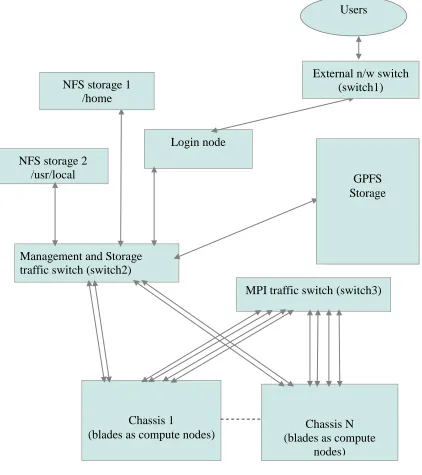
VCL-HPC provides access to two clusters, the Henry2 Cluster and the Sam cluster [2]. We will discuss the Henry2 cluster since we have used the LSF queues configured on the Henry2 cluster for our experimentation. The architecture of the Henry2 cluster is shown in Figure 1. There is a principal login node, and possibly host of on-demand secondary login nodes used for real-time monitoring of specific runs. Login nodes use NFS attached files, and GPFS files to provide data storage. Each computational node has two communication interfaces – an MPI message exchange interface, and a back-end management interface. Typically node interconnects are 1Gbps capable, but more recently 10Gbps sub-clusters have been added. Also there are InfiniBand capable VCL-HPC sub-clusters. Figure 1 illustrates the VCL-HPC architecture.

i. Login nodes:

These are the nodes the users log into from the outside, compile their code on, and invoke LSF scheduler from (submit jobs to Henry2 queues) [98]. A login node has two network interfaces, one interface connects to the external world via the switch1 in Figure 1 and the second interface, which is connected to switch2, provides access the compute nodes and storage. It has access to MVAPICH, MPI, BLAS, etc libraries, as well as Intel (icc, icpc, ifort), GNU (cc, f77) and PGI (pgcc, pgf77, pgf90) compilers, and to other HPC tools. Different queues are configured using LSF to provide mapping among user groups and hardware groups.

ii. Network:

(27)

support about 1344 nodes (this is an approximate number because some of the chassis have separate low latency networks and have a single Gigabit Ethernet link to the core message passing switch). Communications between compute nodes may be non-uniform due to Henry2's network architecture. Nodes within a single chassis can communicate with no bandwidth restriction (full gigabit in each direction) via the chassis backplane. Communications between blades in different chasses is limited to 4 gigabits per second in each direction. So for example if eight nodes in one chassis were exchanging messages with eight nodes in another chassis they could each potentially have a gigabit per second of traffic in each direction for total of 8 gigabits of data per second in each direction. However the Henry2 network architecture would limit the achievable communication rate to four gigabits per second in each direction. The communication could also be impacted by message passing network traffic from the other blades in each chassis that share the aggregated links. In addition to the bandwidth effects of the network design there are also latency effects. Within a chassis messages have a single switch to traverse. For communications between chasses there are three switches that must be traversed (the chassis switch in each chassis plus the core switch). Each network switch adds some additional time before a message reaches its destination [99]”.

iii. Storage:

(28)

accessing large numbers of small files. GPFS as configured on Henry2 uses four servers that create network shared disks (NSDs). These NSDs create a file system that is mounted on each Henry2 login and compute node. GPFS input/output (I/O) operations are cached on the local node and then synchronized with the file system. Multiple NSD servers are able to support more concurrent use and also provide resiliency against failures [99]”.

iv. Nodes:

“Computational nodes are typically IBM BladeServer blades. Each node runs CentOS release 5.4, and has access to appropriate math, MVAPICH, and MPI libraries and various compilers. Henry2 nodes are typically dual Xeon blade servers. But, there are a mix of single-, dual-, and quad-core Xeon processors. Nodes typically have 2-3GB of memory per processor core and a modest size disk drive that is used to hold the operating system, swap space, and a small local scratch space. Nodes have two Gigabit Ethernet interfaces (10 Gbps in some chasses). In compute nodes one of these interfaces is used for a private network connecting the compute nodes to the login nodes and to cluster storage resources. The second Gigabit Ethernet interface is used for a private network dedicated to message passing traffic. On login nodes one interface is used for access from the Internet and the second for access to compute nodes and storage [99]”.

2.2 ARC: A Root Cluster for Research into Scalable Computer Systems

(29)

ARC cluster architecture:

The internal architecture of the GPGPU ARC cluster at NC State is as shown in Figure 2. It consists of a head node, a login node, network switch and 108 node cluster of 1U SuperMicro nodes with one nVidia GPU per node. The nodes have one Mellanox InfiniBand adapter card each (configured at 40Gb/s). They are connected to each other via Mellanox InfiniScale switches Description and purpose of each component follows:

i. Head Node:

Head node is the main interface to the outside world and the users. The users login to the head node and are automatically redirected to the cluster login node. The PBS server daemon runs on the head node. The head node (pbs server) is responsible for scheduling, queuing and forwarding of the jobs to the computational nodes in the GPGPU cluster. Jobs are submitted via the PBS (Maui scheduler). As soon as the job is queued, the head node (using Maui scheduler) looks for the first unused GPU node in the cluster (or for the total number of nodes requested by the user) and sends the job over to the node to be executed. The granularity of access is a node and not a single core as is the case with the LSF scheduler in the Henry2 cluster. The scheduler controls the job queuing time and has control over the execution time. If a job takes more than the allocated time the job is killed and the node is freed to execute new jobs.

ii. Firewall:

The entire cluster is managed by Rocks [5] and is firewalled from the outside. Rocks, requires the cluster to be on a private network. Rocks, discovers computational nodes over Ethernet and installs Linux on the local hard drive of these nodes over PXE. The head node is outside the firewall to allow users to get to the login node. One needs to be in the college network to access the ARC cluster.

iii. Login Node:

(30)

pgf77, pgf95, pgCC) compilers and other tools are installed. The user is responsible for any other required libraries if those are required. The login node is the same in hardware configuration (see Table 2) as the 108 other cluster compute nodes, except that it does not take part in any compute activities. PBS client is not installed on this machine and hence the PBS server cannot send jobs to this machine. Login node has a GPU unit attached to it so as to enable users to compile CUDA based code. Once the code is compiled on the login node, it is submitted to the scheduler queue using the PBS (Maui) commands (qsub command). Details on how to get started, compile the code and submit jobs to the scheduler can be found on the website [3].

iv. NFS Attached Storage

ARC users have all their data on the login server assigned to them. Data is made available to computational nodes via NFS.

v. Computational nodes:

Each node has a GPGPU unit (nVidia GPU card) as well as the runtime libraries required to execute user applications. The Maui scheduler (pbs_server) running on the head node selects one of these nodes (or the number of nodes requested by the user) to schedule the job.. Each node has a 120 GB SSD drive to boost the performance even further. Some nodes differ in the type of GPU card installed on them. The various GPU cards available are nVidia C2070, nVidia C2050 and nVidia GTX480 [3]. Access to different GPU card groups is controlled through scheduler queues.

(31)

Figure 2: Arc Cluster PBS/Torque

resource manager, Scheduler

(Muai/Moab)

User redirection

Cluster of 108 compute nodes with on GPU per node Head Node

(pbs_server)

Login Node

N/w Switch

InfiniBand Switch Firewall

NFS storage

Users

(32)

2.2 General Purpose User Defined Clusters in VCL

We also have designed a user defined cluster using VCL general purposes resources. These resources are provisioned by the VCL management node and a user may not have control over the configuration topology or computational node profiles beyond general infrastructure characteristics such as the type of operating system on the node and CPU speed.

2.2.1 VCL Compute Cluster using Torque resource manager and Maui scheduler

Figure 3 illustrates the overall view of a general user constructed cluster in VCL (in this case comprised of 5 nodes). The user can request resources from VCL, via the user web interface, either individually (one node at the time) or using cluster reservation option. In either case, these resources are normal VCL resources, such as Linux based machines (CentOS 5.4), except that they may be logically structured as shown in Figure 3. Depending on the user privileges, it may be possible to request the resources to be within a particular rack or chassis and to have particular characteristics. However, in most cases, the resources may come from anywhere in the VCL cloud (even different data centers). This will impact physical topology of the network interconnects and homogeneity of the provisioned computational resources.

There is a head node which runs whatever the user installs on it – for example in our example case, Torque (pbs_server) resource manager [68] with a Maui scheduler [69] (pbs_mom) on Linux. The other nodes run as worker nodes or basic compute nodes. The head node, which also acts as a login node, distributes jobs to the compute nodes. All the nodes have the OpenMPI configured

As an example, simple jobs submission to pbs_server would look like this $> echo “Nikhil” | qsub

(33)

This starts a job on four nodes and provides the user with an interactive shell in one of the nodes. Jobs can now be launched using the command:

$> mpirun -np 4 ./executible

More complex jobs can be submitted by writing a PBS script. More information can be found on the Torque website [68].

Following steps need to be followed to setup a general purpose cluster (five node cluster):  Request five reservations for similar machines from VCL

 Setup ssh keys between the VCL nodes so that they can talk to each other securely and without using passwords.

 Setup ssh keys for root as well as the user who is going to run the jobs in the end.  Setup a DNS service of some kind for the nodes. This can be done by either

leveraging normal VCL DNS services and/or by adding entries to the /etc/hosts file. We have used the /etc/hosts file method.

 Setup a shared storage between these servers via NFS or any NAS solution available.  Open the firewall ports that Torque and Maui use.

 Download and install Torque or PBS on head node (pbs_server)

 Configure the head node and the compute nodes in Torque configuration files  Install the PBS compute node packages on the slave nodes (pbs_mom)

 Download and install the Maui scheduler service on the head node

 Start the PBS and the Maui services on the Head node as well as the compute nodes.  At this point the compute nodes should be seen as “pbsnodes” on the Head node.  Install the Torque aware OpenMPI library on the Head node.

 Share this library over the shared storage and change library and default paths to point to this shared storage.

 Now, the cluster is ready to execute MPI jobs

(34)

Figure 3: HPC in VCL (VCL-GP) Custom HPC Cluster in VCL

Head Node (pbs_server/maui) Compute node 1 (pbs_mom)

VCL Management node – VCL subsystem User

Compute Node 2 (pbs_mom)

(35)

2.3 A discussion of Hadoop cluster on VCL nodes

Depending on the interconnect topology and nodes, one may be able to use the on-demand cluster as a more tightly coupled HPC cluster, or perhaps as an High Performance Data (HPD) cluster, or a general loosely coupled computational engine., HPD is concerned with intelligent data distribution so that applications can take advantage of data parallelism. Map reduce techniques have been instrumental in achieving good performance for applications working on highly parallel and distributed data. The essence hinges on high parallelism for large but almost independent data sets (such as those found in the context of unstructured data sets/files that need to be independently searched) and on relatively low intensity low latency sensitivity inter-node communication traffic levels Apache Hadoop [71] is an open source implementation of the Map-Reduce approach. The Apache Hadoop software library is a framework that allows for the distributed processing of large data sets across clusters of computers using a simple programming model [71]. The Hadoop library can work on jobs with data sets on a single machine to thousands of machines. Hadoop provides various features like high availability, fail-over techniques, load balancing, etc. The HDFS (Hadoop Distributed File System) distributes the application data to achieve the required scalability. Since the application data placement is handled by the HDFS layer, it has the capability to distribute and locate the application data as requested thus the paradigm of Map Reduce can now be applied to the application data using a simple programming model.

(36)

(37)

Chapter 3 Performance

3.1 The LINPACK Benchmark

The LINPACK Benchmark was introduced by Jack Dongarra et al. in 1979 [26]. It is available from at [10]. “The Linpack Benchmark is something that grew out of the Linpack software project. It was originally intended to give users of the package a feeling for how long it would take to solve certain numerical problems. The benchmark stated as an appendix to the Linpack Users' Guide and has grown considerably since the first Linpack User’s Guide was published in 1979 [55]”.

(38)

LINPACK measures the performance of an HPC cluster by calculating the number of floating point operations per second or FLOPS the cluster can perform. The performance is generally reported in millions of floating point operations per second or gigaflops per second. The Top500 [44] community reports the performance in MFLOPS or mega floating point operations per second.

3.1.1 High Performance LINPACK (HPL)

High Performance Linpack (HPL) [10] is the parallel and unrestricted version (size of coefficient matrix is flexible and can be changed manually) of the LINPACK benchmark (LINPACK100 [55], LINPACK1000 [85]) which solves a random dense linear system of equations. HPL performs double precision (64 bits, 8 bytes) arithmetic on distributed-memory computers. HPL is a portable open source implementation of the High Performance Computing Linpack Benchmark [10].

The algorithm used by HPL can be summarized by the following keywords: “Two-dimensional block-cyclic data distribution - Right-looking variant of the LU factorization with row partial pivoting featuring multiple look-ahead depths - Recursive panel factorization with pivot search and column broadcast combined - Various virtual panel broadcast topologies - bandwidth reducing swap-broadcast algorithm - backward substitution with look-ahead of depth one” [10].

The output of HPL [10] provides values for accuracy, detailed timing, the total computation time required and the performance in GFLOPS (Floating point operations per second). HPL requires Message Passing Interface MPI, Basic Linear Algebra Subprograms BLAS or Vector Signal Image Processing Library VSIPL libraries installed on the system [10].

3.1.1.1 HPL algorithm

(39)

[[L,U] y]. Since the lower triangular factor L is applied to b as the factorization progresses, the solution x is obtained by solving the upper triangular system U x = y. The lower triangular matrix L is left unpivoted and the array of pivots is not returned” [10].

 “The data is distributed onto a two-dimensional P-by-Q grid of processes according to the block-cyclic scheme to ensure "good" load balance as well as the scalability of the algorithm. The n-by-n+1 coefficient matrix is first logically partitioned into nb-by-nb blocks, that are cyclically "dealt" onto the P-by-Q process grid. This is done in both dimensions of the matrix” [10].

 “The right-looking variant has been chosen for the main loop of the LU factorization. This means that at each iteration of the loop a panel of nb columns is factorized, and the trailing submatrix is updated. Note that this computation is thus logically partitioned with the same block size nb that was used for the data distribution” [10].

3.1.1.2 HPL performance tuning parameters

The various tuning parameters are available in the HPL.dat file. Following are some of the parameters:

 N's: This is the problem size. These values indicate the order of the coefficient matrix. The bigger the matrix size, more the floating point operations. For better performance, the matrix needs to fit in the physical memory of the machine [10].  NB: NB is the block size. It is basically the block size used during the LU block

factorization of the matrix. A parallel LU algorithm calculates the LU factorization with block granularity and this factor determines the block size for factorization [10].  P,Q: P: Rows in process grid. Q: Columns in process grid

(40)

Parameters not considered in this scenario:

 “Depth: This factor specifies the look-ahead depth used by HPL. A depth of 0 means that the next panel is factorized after the update by the current panel is completely finished. A depth of 1 means that the next panel is immediately factorized after being updated. The update by the current panel is then finished [10].

 BCASTS: In the main loop of the algorithm, the current panel of column is broadcast in process rows using a virtual ring topology. HPL offers various choices and one most likely want to use the increasing ring modified encoded as 1. 3 and 4 are also good choices [10].

 RFACTS, PFACTS, NDIV, NBMIN: These parameters specify the algorithmic features. HPL will run all possible combinations of those for each problem size, block size, process grid combination. This is handy when one looks for an "optimal" set of parameters. To understand a little bit better, let say first a few words about the algorithm implemented in HPL. Basically this is a right-looking version with row-partial pivoting. The panel factorization is matrix-matrix operation based and recursive, dividing the panel into NDIV subpanels at each step. This part of the panel factorization is denoted below by "recursive panel fact. (RFACT)". The recursion stops when the current panel is made of less than or equal to NBMIN columns. At that point, xhpl uses a matrix-vector operation based factorization denoted below by "PFACTs". Classic recursion would then use NDIV=2, NBMIN=1. There are essentially 3 numerically equivalent LU factorization algorithm variants (left-looking, Crout and right-looking). In HPL, one can choose every one of those for the RFACT, as well as the PFACT [10].

(41)

few order of magnitude bigger than 1 for example 10^6 or more. Note: if one was to specify a threshold of 0.0, all tests would be flagged as failed, even though the answer is likely to be correct. It is allowed to specify a negative value for this threshold, in which case the checks will be by-passed, no matter what the threshold value is, as soon as it is negative. This feature allows to save time when performing a lot of experiments, say for instance during the tuning phase. Example: -16.0 threshold [10].  Swap: This parameter allows specifying the swapping algorithm used by HPL for all

tests. There are currently two swapping algorithms available, one based on "binary exchange" and the other one based on a "spread-roll" procedure (also called "long" below). For large problem sizes, this last one is likely to be more efficient [10].

 L1,U: This parameter specifies whether the upper triangle or the panel of rows is stored in transpose for or not [10].

 Align: This parameter allows specifying the alignment in memory for the memory space allocated by HPL. On modern machines, one probably wants to use 4, 8 or 16. This may result in a tiny amount of memory wasted [10]”.

HPL was executed on the clusters mentioned in the previous chapter and the performance of HPL on different clusters is presented in the following sections. Cluster configurations are identified below along with the results.

Some HPL runs were done on single core processors, and some were done on multi core processors. Single core runs for sample configurations are given in Appendix B as is a possible theoretical limit on the performance of a processor core. The processor performance depends on various factors which are very much related to the microprocessor architecture and the test being run. Asim Nisar et al. in [94] give a deeper insight on the factors that affect performance for a 45nm Core2 processor.

(42)

similar architecture and network interconnects. However, the resource manager maintains different job queues for different hardware/platforms. The resource manager does not guarantee that the job will run on the same machine every time. The job can run on different machines (e.g: different core architectures) at different times but belonging to the same queue and having the same or very similar hardware and software configuration.

3.2 Performance evaluation of compute jobs on VCL-GP nodes

A possible VCL node configuration is shown in Table 1 below. All the results were taken on nodes with similar configuration. Various tests were run in order to characterize components of this cluster, and composites of these components, with regards to performance. This includes CPU utilization stats.

Table 1: CPU Configuration 1: A typical node in VCL-GP cluster

Cluster VCL cluster

Queue Batch

Processor Model Xeon L5638

Microprocessor Architecture Westmere-EP

Clock Frequency 2 GHz

Number of Processors 1

Number of Cores 1

Hyper threading NO

L1 cache 32k-Instr, 32k data per core

L2 cache 256K-Unified per core

L3 cache 12288K-Unified per processor

Memory 1 GBytes

Network 1 G Ethernet

Operating System CentOS release 5.4 (Final)

OS architecture X_86, i686

I. HPL Single node test:

(43)

by adding more nodes we might get better performance. This is explored in the next section where we test the performance of HPL on an on-demand cluster of VCL-GP nodes.

Figure 4: HPL results for varying blocksize on a single VCL-GP node (1 core)

II. Four node VCL-GP Cluster using HPL with varying Matrix size (N):

We constructed a four computational node cluster using VCL-GP nodes (of the same type as in I above). The maximum performance achieved by HPL tests with varying Matrix sizes is shown in Figure 5 (horizontal axis is the matrix size (time at which the test was run) (blocksize at which the maximum performance for this matrix size was observed) and vertical axis show the performance in GFLOPS). Note that in the figure, at all four times the same reservation (same 4 node cluster) exists, but T1 and T2 were nearly 2 days apart (T1 for 10000 order matrix took more than a day to complete). T3 was performed the same day after T2 and T4 was performed a week later T3.

(44)

As we can see in the Figure 5 that increasing the matrix size tends to increases the performance. As we increase the matrix size, we fill the processor pipeline with more floats. This ensures that there is little or no idle time for the processor. Increasing the Matrix size also makes sure that the processor pipeline has fewer bubbles. Since HPL takes advantage of temporal as well as spatial locality of data (spatial locality is not as highly exploited as temporal locality in HPL), the more data fills up the cache, and the larger is the floating point rate. However, this holds only up to a point. There might be a stage where increasing the matrix size degrades the performance.

For example, with reference to Figure 5, at time T1 the performance increases with the increase in the matrix size. However performance degrades for matrix size of 10000. At time T3, we observed that the performance increases until matrix size 10000, in fact it reaches up to 18 GFLOPS on a four node cluster and an average aggregate performance of about 4.5 GFLOPS per processor. Note that this graph shows the maximum performance from all the tests. The maximum performance was observed at different block sizes for different matrix sizes, at different times as shown in the figure.

Figure 5: Maximum HPL performance for varying matrix size (N) (blocksize (NB) at which max performance was observed is noted). (Test: 4 nodes, 4 cores). Measurements were taken

(45)

III. HPL with varying blocksize (NB):

Results of HPL on VCL-GP (4 node cluster) with varying block are shown in Figure 6. The horizontal axis represents blocksize and vertical axis represents performance in GFLOPS. The results measured at different times produced different results due to, for most part, the difference in network bandwidth at different times. We see that increasing the block size increases the performance up to a maximum point. Further increase in the block size causes degradation in performance. It can be argued that as we increase the block size, we increase the advantages of temporal locality. But if we go on increasing the block size, the advantage of data parallelism is lost and hence we see degradation in performance.

It was also observed that larger blocksize can perform better on bigger matrices. This is because in a bigger matrix, there is a larger scope to take advantage of data parallelism. Hence, increasing the blocksize increases the advantages of temporal locality without affecting the data parallelism. The important distinction in this case is that the effect of blocksize followed a similar pattern at two different times T2 and T3. This proves that the HPL algorithm had no glitches but the difference in performance at times T2 and T3 was purely due to configuration related issues (change in network parameters in this case).

(46)

IV. A simple analysis of the Ping-Pong benchmark results:

Ping-pong, a test in the HPCC suite of benchmarks [105], provides a measure of network bandwidth and latency of MPI messages. The latency graph as shown in Figure 7 (horizontal axis represents time (order of matrix used for the test) and the vertical axis represents the Ping Pong MPI latency for 8 byte messages in milliseconds, the latencies map to left hand scale while the performance maps to the right hand scale. The performance always maps to the right hand scale henceforth). It shows that the Ping Pong latency for 8 Byte messages was almost constant at different times and in the 0.06 to 0.09 ms range while the natural order and random order latencies were in the range of 0.05 to 0.07 milliseconds.

However, it is interesting to note that the bandwidth observed at different times was different. As shown in Figure 8 (horizontal axis represents time (order of matrix used for the test) and vertical axis represent the network bandwidth in MegaBytes/second), the bandwidth at times T1, T2 and T3/T4 goes on increasing respectively. This seems to be reflected, in part, in the performance of HPL as shown in Figure 5. The performance at time T3 was the maximum peak performance achieved. Although the latency for 8 Byte messages hardly varied (0.06 to 0.09 ms range), there were changes observed in network bandwidth. Network bandwidth is exploited when large data sets are transferred over the network. In a Ping Pong test the bandwidth is high when 2,000,000 Byte messages are sent across. Similarly, when dealing with larger matrix sizes large data sets are transferred across the network which is why we see a difference in the overall performance.

(47)

Figure 7: Ping-Pong network (MPI) latency, (Test: 8 Byte message, 4 nodes, 4 cores, T1, T2

 T1+2 days and T3 T2 + 2 hours, T4  T3 + a week)

Figure 8: Ping-Pong network (MPI) bandwidth, (Test: 2MB messages, 4 nodes, 4 cores, T1, T2  T1+2 days and T3 T2 + 2 hours, T4  T3 + a week)

V. HPL performance on single node and multi-node configuration:

(48)

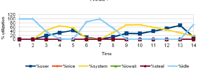
Figure 9: CPU utilization of a VCL node in the cluster, (Test: 4 nodes, 4 cores). Relative time on the x-axis is in seconds.

We see that the neither system CPU utilization (network stack processing) nor the user CPU utilization (floating point computations) exceeds about 60%. The compute processes appears to get less than 60% of the CPU time.

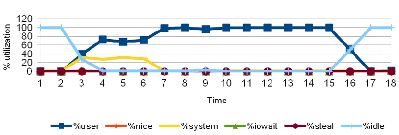
The results of a similar test with HPL being run on a single node with no network packets is shown in Figure 10 (horizontal axis represents relative time with interval of 1 seconds and vertical axis represent the percentage utilization of CPU) depicts that the processor was utilized to its full potential and just for computations. The user process (HPL computations) executes on the CPU with 100% utilization when the test was running. The difference in performance in the above graphs proves that HPC in cloud cannot guarantee performance stability. These observations bring out an important conclusion that HPC in cloud is not perfect.

For the VCL-GP tests the following version of compilers and libraries were used. Open-MPI version: 1.4.5

(49)

Mpicc version: gcc (GCC) 4.1.2 HPL code available from [105]

GotoBlas2 math library: Optimized GotoBLAS2 libraries version 1.13 available from [90] CC FLAGS: -fomit-frame-pointer -O3 -funroll-loops -Wall

Figure 10: CPU utilization, single node test (1 core)

3.3 Performance evaluation of compute jobs on ARC cluster

ARC cluster was described in Chapter 2. For the ARC cluster tests the following version of compilers and libraries were used.

Open-MPI version: 1.5.4 Rocks: 5.3 (Rolled Tacos) HPL code available from [105]

HPL-GPU code available from the NVIDIA Developer site [21] (The HPL algorithm for CPU+GPU and implementation is described in the paper [22])

Mpicc version: gcc (GCC) 4.1.2

GotoBlas2 math library: Optimized GotoBLAS2 libraries version 1.13 available from [90] HPL CC FLAGS: -fomit-frame-pointer -O3 -funroll-loops –Wall

CUDA toolkit version: 4.1 (RC1)

(50)

HPL-GPU CC FLAGS: -fomit-frame-pointer -W -Wall -fopenmp –g

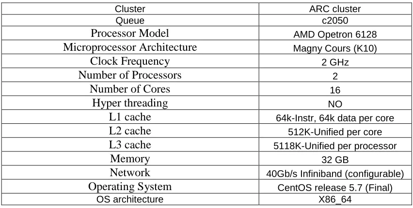
Table 2: CPU Configuration 2: A node in the ARC cluster

Cluster ARC cluster

Queue c2050

Processor Model AMD Opetron 6128

Microprocessor Architecture Magny Cours (K10)

Clock Frequency 2 GHz

Number of Processors 2

Number of Cores 16

Hyper threading NO

L1 cache 64k-Instr, 64k data per core

L2 cache 512K-Unified per core

L3 cache 5118K-Unified per processor

Memory 32 GB

Network 40Gb/s Infiniband (configurable)

Operating System CentOS release 5.7 (Final)

OS architecture X86_64

3.3.1 CPU cluster performance characterization

Following tests were performed to characterize the CPU performance of the ARC cluster.

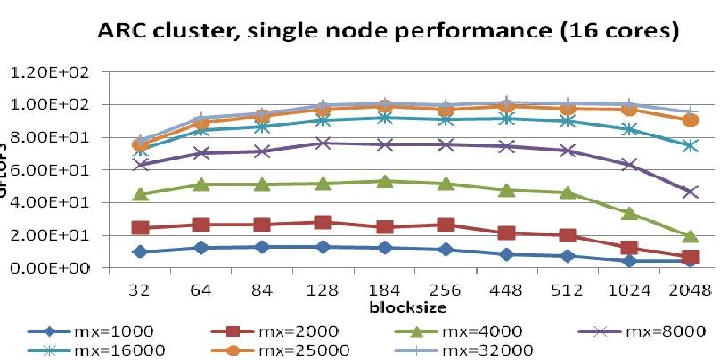
I. HPL performance on a single node in ARC cluster:

(51)

Figure 11: HPL Performance, 1 node (16 cores)

II. HPL with varying Matrix size and blocksize (N, NB):

Figure 12 (horizontal axis represent varying blocksize and vertical axis represents performance in GFLOPS), illustrates that as we go on increasing the Matrix size the performance increases. This is because of the linear scaling of the HPL algorithm. With increasing block sizes, we see that a point of maximum performance is reached, and then the performance drops. The point of maximum performance is different for different Matrix sizes. For a 64,000 ordered matrix, the performance starts degrading for blocksize 84 and keeps dropping for larger blocks. For order 32,000 matrix, the performance drops after blocksize of 184. The graph does not give a clear single point of maximum for all the tests. But the important fact to note is that as we increase the blocksize to 84, we see an incline upwards in all the graphs, which means that the performance increases when blocksize is increased from 32 to 84. From blocksize 84 to 184, the performance is fluctuating, but after blocksize 256, the performance degrades for all the graphs. Similar observations were seen when the test was run on increasing number of processors.

(52)

128 cores, since each node in the ARC cluster has 16 cores as shown in Table 2. This is because, in this configuration, by default, the OMP_NUM_THREADS value is set to the total number of cores on each node.

Figure 12: HPL Performance, 8 node (128 cores)

III. HPL with varying the process grid mappings (P and Q):

(53)

As we increase the matrix size to 32,000 or 64,000, we see a difference. For order 64,000 matrix, the performance for P=2 and Q=4 was observed to be the best. It is interesting to note that both P and Q were powers of two. For larger matrices, the grid mappings which are a power of two perform better. Similar results were observed for 32,000 ordered matrix

Figure 13: Effect of grid mappings, 8 node (128 cores), Matrix size=1000

(54)

Figure 15: Effect of grid mappings, 8 node (128 cores), Matrix size=64000

IV. A simple analysis of the Ping-Pong benchmark results:

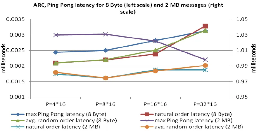
The latency-bandwidth test was done to measure the difference in latency or bandwidth when we increase the number of MPI processes. As shown in the Figure 16 (horizontal axis represent different configuration of processes and the left vertical axis represent the latency for 8 Byte messages in milliseconds and the right vertical axis represent the latency for 2 MB messages in milliseconds), the latency increases with increase in the total number of processes with the exception that the maximum Ping Pong latency for an 2 MB message decreases with increase in number of processes. Although there is slight increase or decrease in latency, the difference is not large enough to affect the performance. In fact, increasing the total number of processes increases the total performance on the ARC cluster. As seen in the bandwidth test in Figure 17 (horizontal axis represent different configuration of processes and the vertical axis represent the network bandwidth in MB/s), the bandwidth distribution is almost in harmony with the latency test. The minimum Ping Pong bandwidth increases slightly but overall the minimum bandwidth achieved is within the range 1940 to 2000 MB/s.

(55)

two nodes in a distributed system talk to each other directly or when ordered in a ring structure. The minimum, average and maximum bandwidth and latency reported by Ping Pong is shown in Table 3.

Figure 16: Ping pong latency, 8 node (128 cores, 8 Byte message and 2 MB message)

(56)

Table 3: Ping Pong Min/Avg/Max bandwidth and latency (ARC cluster) Process

configuration 2 MB message bandwidth (MB/s) 8 Byte Latency (milliseconds) 2 MB latency (milliseconds) (P=nodes*pr

ocsper node) min avg max min avg max min Avg max

P=4*16 1941.81 1990.99 2038.79 0.00218 0.0024 0.0024 0.98097 1.0048 1.03

P=8*16 1939.79 2043.05 2362.66 0.00212 0.0024 0.0025 0.84651 0.9819 1.031

P=16*16 1956.98 2084.58 2443.52 0.00225 0.0025 0.0028 0.81849 0.9623 1.022

P=32*16 2003.97 2318.17 2717.4 0.00231 0.0027 0.0031 0.736 0.8664 0.998

V. Interesting results and observations:

We also executed a test to explore the peak performance of the ARC cluster. Unfortunately we could only reserve a maximum of 32 nodes. As discussed previously, the peak performance was observed when the block size is in the range of 64 to 128. The interesting fact to note is that the peak performance achieved was 2.23 TFLOPS with 512 cores as shown in Figure 18 (the horizontal axis represent varying blocksize and vertical axis represents performance in GFLOPS). Assuming a balanced distribution of workload by HPL, this indicates that the performance of around 4.5 GFLOPS was achieved per core. With MPI traffic on the InfiniBand interconnects, we could achieve 4.5 GFLOPS per core. An interesting topic for further research would be to examine this with a larger number of processes. These tests would reveal whether the CPU utilization and the performance continue to increase or not.

(57)

GigE with 7236 cores which gives 50.9 TFLOPS. If the ARC cluster is expanded to around 800 nodes, we might be able to get to the Top500 list (this may or may not be true since the relative utilization drops as we go on increasing the number of processes).

Figure 18: ARC cluster Peak Performance, 32 nodes (512 cores)

But this is not possible for an in-house cluster. If somehow we could attach 800 more nodes to the ARC cluster on the fly, requesting these resources from a cloud subsystem, we will have a supercomputer at NC State. Thus, more reasons to explore HPC in cloud.

(58)

3.3.2 CPU and GPGPU cluster performance characterization (ARC, CPU+GPU)

LINPACK was initially developed in Fortran but later as LINPACK became widely used, a C version was developed. To test the performance of NVVIDIA GPGPU's, NVIDIA has developed a new CUDA based version of HPL. It is available from [21]. For the experiment we use the CUDA compatible HPL (version 1.3), cuBLAS library (version 4.1.21) and OpenMPI (version 1.5.4) libraries (more details are given at the beginning of section 3.3).

Even though ARC is a specialized cluster used for GPGPU workloads, the CPU characterization in the earlier section raises an important issue, is GPGPU a necessity? In the following section we discuss some of the performance numbers when HPL was run on CPU versus when HPL was run on CPU+GPU. The CUDA based HPL is tested on the ARC cluster. Configuration of the GPU card on a node in the ARC cluster is explained in Table 4 and 5.

Table 4: Configuration of a GPGPU card in the ARC cluster [3]

Cluster ARC cluster

Queue c2050

GPGPU Model NVIDIA C2050 Tesla card

Microprocessor Architecture Fermi

Clock Frequency (Core/Shader/Memory) 575/1150/3000 MHz

Number of GPU cards 1

Number of Cores/Stream processors 448

Hyper threading NO

Theoretical Peak Performance 515 Gflops

L1 cache (per SM) Configurable 16 KB or 48 KB

L2 cache 768KB

L3 cache No

Memory 32 GB

Network

40G Infiniband/ PCI-E for CPU to GPU interconnect Operating System CentOS release 5.7 (Final)

(59)

Table 5: Configuration of Tesla C2050 GPU card (used in the experiments) [91]

GPU Fermi (c2050)

Transistors 3.0 billion

CUDA Cores 512

Double Precision Floating Point Capability 256 FMA ops /clock

Single Precision Floating Point Capability 512 FMA ops /clock

Special Function Units (SFUs) / SM 4

Warp schedulers (per SM) 2

Shared Memory (per SM) Configurable 48 KB or 16 KB

L1 Cache (per SM) Configurable 16 KB or 48 KB

L2 Cache 768 KB

ECC Memory Support Yes

Concurrent Kernels Up to 16

Load/Store Address Width 64-bit

I. HPL performance on a single node with CPU+GPU:

As seen in the graph in Figure 20 (the horizontal axis represent varying blocksize and vertical axis represents performance in GFLOPS), a single node CPU+GPU could deliver around 268 GFLOPS. From the results in Figure 11 and 20, we observe that the performance achieved by a single core CPU plus a 448 core GPU together, is more than twice when compared to a standalone CPU system with 16 cores. Thus a GPGPU is important when compared to processing power contained in a single node.

High-Performance Cloud Computing: VCL Case Study.

DEDICATION

BIOGRAPHY

ACKNOWLEDGMENTS

TABLE OF CONTENTS

LIST OF TABLES

LIST OF FIGURES

Chapter 1

Introduction

Chapter 2

NCSU HPC Resources

Chapter 3

Performance