Implementation of Genetic Algorithms and Parallel Simulated Annealing in OCEON-P

Abstract

DU, SHUANG. Implementation of Genetic Algorithms and Parallel Simulated Annealing in OCEON-P. (Under the direction of Paul J. Turinsky).

OCEON-P is a computer program whose purpose is to minimize the levelized fuel cycle cost over a multi-cycle planning horizon. It integrates a core simulator, fuel cycle cost calculator and mathematical optimization engine. The accuracy of the predicted fuel cycle cost, whose minimization guides the optimization of the decision variables, is directly related to the fidelity of the reactor core simulator used by the program. Unfortunately, high fidelity core simulators also require longer run times. To improve these run times, this project sought to parallelize the optimization process so that multiple processors may share the

computational burden. In addition, an effort was made to reduce the number of fuel cycles that must be examined to complete the optimization, which also reduces the computer run times.

Implementation of Genetic Algorithms and Parallel Simulated Annealing in OCEON-P

by Shuang Du

A thesis submitted to the Graduate Faculty of North Carolina State University

in partial fulfillment of the requirements for the Degree of

Master of Science

Nuclear Engineering

Raleigh, North Carolina 2008

APPROVED BY:

_________________________ _________________________ Dr. Dmitry Y. Anistratov Dr. Moody T. Chu

________________________________ Paul J. Turinsky

Biography

Shuang Du was born on the twenty-second of June 1985. He received his grammar school education in Hawaii, California, and North Carolina, eventually graduating from Apex High School ranked second in a class of 447. It was also in high school that Shuang obtained his American citizenship.

In 2003 Shuang enrolled in the Department of Nuclear Engineering at North Carolina State University supported completely by scholarships at the departmental, college, and University levels. Of particular note was an undergraduate fellowship from the Department of Homeland Security obtained during the junior year which generously provided a monthly stipend as well as full tuition and fees. During his college education Shuang has completed internships at both Los Alamos National Laboratories and Lawrence Livermore National Laboratories.

Acknowledgements

I would like to thank the many people who have made it possible for me to reach this point. Firstly I would like to thank Professor Paul Turinsky, whose invaluable guidance and patience saw me through this process. Furthermore, I am very grateful towards Professors Chu and Anistratov for taking time out of their busy schedules to be on my graduate

committee. In addition, I would also like to thank Duke Energy for supporting this project. At Duke Energy, I would like to thank Bob Harvey for his direction, John Bartels for his project related wisdom, and everyone else on the team for their support.

Table of Contents

LIST OF TABLES ……… v

LIST OF FIGURES ……… vi

INTRODUCTION ……… 1

Out-of Core Fuel Management Optimization ……… 1

Background ……… 1

Cost Components ……… 1

Design Constraints ……… 2

Design Decisions ……… 3

Historical Approach ……… 3

Scope of Research ……… 4

Review of Current Optimization Techniques ……… 5

Genetic Algorithms ……… 5

Parallel Simulated Annealing ……… 8

METHODOLOGIES ……… 10

Genetic Algorithms ……… 10

Crossover Type ……… 10

Initial Population ……… 11

Soft Constraints in Genetic Algorithms ……… 12

Selection ……… 15

Archiving and Elitism ……… 20

Probability Distributions for Feed Size Selection ……… 21

Crowding and Niching ……… 22

Tuning Parameter Optimization ……… 24

Parallel Simulated Annealing ……… 31

Exchange of Information ……… 31

MPI Overhead ……… 33

RESULTS ……… 36

Genetic Algorithm Results ……… 36

Parallel Simulated Annealing Results ……… 40

CONCLUSIONS AND FUTURE WORK ……… 41

Conclusions ……… 41

Recommendations for Future Work ……… 41

List of Tables

Table 2.1: Energy production schedule used ………. 10

Table 2.2: Comparison of crossover types ………. 11

Table 2.3: Example of possible feed region sizes ……… 12

Table 2.4: OCEON-P violation types ………. 13

Table 2.5: Scaling type result comparison ………. 20

Table 2.6: Archiving implementation ……… 21

Table 2.7: Niche control implementation ……… 24

Table 3.1: Parameters used for final GA study ………. 36

List of Figures

Figure 2.1: Comparison of crossover types ……… 11

Figure 2.2: First-order scaling domain ……… 16

Figure 2.3: First-order domain violation range ……… 17

Figure 2.4: Second-order probability distribution ……… 18

Figure 2.5: Second-order domain violation range ……… 18

Figure 2.6: Scaling domain comparison ……… 19

Figure 2.7: Scaling type result comparison ……… 20

Figure 2.8: Niche control implementation ……… 24

Figure 2.9: FCC sensitivity to population size ……… 25

Figure 2.10: FCC standard deviation with changing population sizes ……… 26

Figure 2.11: FCC sensitivity to crossover probability ……… 26

Figure 2.12: FCC standard deviations with changing crossover probability 27

Figure 2.13: FCC sensitivity to mutation probability ……… 27

Figure 2.14: FCC standard deviation with mutation probability variation …. 28 Figure 2.15: FCC sensitivity to pressure variation ……….. 28

Figure 2.16: FCC standard deviation with variation in pressure ……… 29

Figure 2.17: FCC sensitivity to elitism percentage ……… 29

Figure 2.18: FCC standard deviation with elitism percentage variation …… 30

Figure 2.19: MPI send latencies ……… 33

Figure 2.20: MPI receive latencies ……… 34

Figure 2.21: MPI overhead ……… 36

Figure 3.1: GA and SA comparison of best solutions found ……… 37

Figure 3.2: SA overall performance ……… 38

Figure 3.3: GA overall performance ……… 38

Figure 3.4: GA and SA convergence behavior ……… 39

1. Introduction

1.1 Out-of-core Fuel Management Optimization 1.1.1 Background

Nuclear fuel management involves making decisions to determine the number of fresh assemblies to be inserted at the beginning of each cycle, the enrichment of these assemblies, as well as where these assemblies are to be placed. In addition, the burnable poison loadings must also be determined. In addition, for boiling water reactors, decisions regarding control rod programming and core flow rate must be made. The objective of nuclear fuel management is to minimize the total cost of creating electrical energy by considering the various components associated thereto. Generally, decisions which affect cost can be broken into in-core decisions, which are made for a particular cycle, and out-of-core decisions, which refer to decisions regarding a multi-cycle planning horizon. Since this project deals with the Out-of-Core Economic Optimization PWR code, henceforth referred to as OCEON-P, only the out-of-core decisions associated with pressurized water reactors will be considered. These decisions are constrained by power limits, fuel burnup limits, reactivity limits, thermal limits, and cycle energy production. Unfortunately, the dependence of the objective constraints on decision variables is non-linear. This means that a closed form mathematical optimization method, such as linear programming, cannot be used. The goals of this project are to attempt to improve the current optimization scheme used in OCEON-P through the use of genetic algorithms and parallel simulated annealing.

1.1.2 Cost Components

The first cost of the nuclear fuel cycle is that which is associated with the mining and milling of uranium. Uranium is procured from parts of the world in which the uranium assay is high enough to justify mining. The raw uranium is then converted and enriched.

The objective of the conversion process is to turn the raw U308 powder into UF6 gas. This is a done via a chemical process. The UF6 is then enriched. The technologies which are used in the enrichment process include gaseous diffusion and gas centrifuge. Newer

available. After the UF6 is enriched, the material is made into a ceramic pellet so that it stays solid and retains fission by-products. These ceramic pellets are then placed in hollow tubes with favorable properties such as low neutron absorption and corrosion resistance. These rods are then bundled together into an assembly and shipped.

When the fuel assembly reaches the reactor, it is loaded during an outage. The assembly is kept in the reactor and the uranium is used to produce electrical energy until the balance in the chain reaction (criticality) cannot be maintained. The fuel is then sent to a spent fuel pool which removes the decay heat from the assembly. If the assembly is not re-used, after five years or some other suitable time for the decay heat to die down, it is placed into dry cask storage. The dry cask is usually cylindrical in shape, made out of steel, and back-filled with inert gas.

This entire process from the mining and milling to the post processing from the spent fuel pool is called the nuclear fuel cycle, more specifically, the open nuclear fuel cycle. Each time the core is refilled, a new cycle begins. The costs associated with each step of the cycle together are called the fuel cycle cost.

1.1.3 Design Constraints

The primary constraints for fuel management that must be satisfied for safety and economic reasons include power limits, fuel burnup limits, reactivity limits, thermal limits and cycle energy production limits.

Power limits deal with peaking factors. Since a reactor can only create as much electricity as its hottest fuel rod and pellet allows, smoother power distributions allow for better utilization of the available fuel without violating thermal limits. Resulting neutron leakage may, however, reduce reload cycle energy production.

Reactivity limits refer to shutdown margin, moderator temperature coefficient, fuel enrichment and soluble boron limits.

Thermal limits deal with the material properties of the fuel assemblies as influenced by heat. These include departure from nuclear boiling, centerline fuel melt, loss of coolant accident limits, and peak clad temperature limits. Most of the time, these limits can be translated into power limits.

The cycle energy production limit is the amount of energy that is expected to be produced per cycle.

1.1.4 Design Decisions

The main design decisions for the out-of-core problem are the number of fresh assemblies to be inserted in each cycle along with their corresponding enrichments, partially burnt fuel to reinsert, and burnable poison loadings. Once these design decisions are made, the remaining decisions become an in-core problem. In-core decisions include placement of fresh and burnt fuel assemblies and burnable poison material. Programs that deal with loading pattern optimization are typically used to obtain an in-core solution. One can see, therefore, that the in-core problem and the out-of-core problem are linked together in that the solution to one must affect the other.

1.1.5 Historical Approach

For in-core nuclear fuel management, nuclear design engineers create the loading pattern for the next reload cycle while satisfying all limits associated thereto. Typically, loading patterns for three subsequent cycles are also determined in this manner. The reason why loading patterns are generated for several subsequent cycles is because it is likely that the choices for loading patterns in the next cycle will affect the performance of three subsequent reload cycles. Additionally, generating the loading pattern for three subsequent reload cycles also gives a better projection of future fuel purchases.

reload cycles are assessed since decisions made for the next reload cycle can impact the out-of-core decisions, objective and some constraints over this number of reload cycles.

1.2 Scope of Research

The OCEON-P computer program tries to find the lowest cost cycle scheme within constraints, i.e. determining decision variable values for a specified planning horizon. The program does this by choosing a cycling scheme, completing depletion simulations and then evaluating the fuel cycle cost and constraints.

One may therefore think of the OCEON-P program as consisting of three parts, the core simulator, the economic engine, and the optimization engine. The core simulator models the depletion of all cycles in the planning horizon, the economic engine calculates the cost of the scheme that was just burned by the core simulator, and the optimization engine chooses the next scheme to be tested such that the search progresses towards the most optimal configuration.

Previous versions of OCEON-P had used a biased integer based Monte Carlo method using hard constraints as the optimization engine. Recently, this method was replaced by Kenney Anderson with simulated annealing combined with soft constraints, which resulted in an increase in the quality and robustness of solutions found by OCEON-P. Simulated

annealing is a serial algorithm, which means that each cycling scheme examined by the core simulator must be assessed one after another. This is not a problem if LRM or FLAC, core simulators used within OCEON-P with low computational requirements, are to be used since tens of thousands of histories can be run in minutes on a PC. However, such core simulators have limited fidelity. Utilities such as Duke Energy use as their reactor core simulator SIMULATE3, a high fidelity core simulator which takes far longer than LRM or FLAC to examine a given cycling scheme. The solution to the long wall clock times associated with SIMULATE3 is a parallel optimization algorithm that can allow multiple computers to share the burden of examining the different cycling schemes while retaining the quality and

Furthermore, an optimization method that reduces the number of cycling schemes that must be examined to achieve a desired level of optimization will also reduce the clock times.

To this end, two new optimization methods which retain the important feature of inherent parallelizability will be implemented and tested. The first optimization method is called Genetic Algorithms, a method which draws its influences on the natural phenomena of survival of the fittest, breeding, and mutation. The second method is parallel simulated annealing, a process similar to serial simulated annealing except for certain fundamental differences which allow it to examine schemes in parallel.

Both these schemes will first be implemented and tested with the version of OCEON-P that uses LRM and FLAC as its core simulators. This is because working with a code that performs runs in minutes rather than days will facilitate the optimization methods’

development and assessment.

The final step is to implement the new method into the version of OCEON-P which uses the SIMULATE3 core simulator.

1.3 Review of Current Optimization Techniques 1.3.1 Genetic Algorithms

The main operators of genetic algorithms are crossover and mutation [8]. The importance of these operators in genetic algorithm theory and implementation has been recognized for some time [1]. Crossover acts as a means through which genes can be swapped by parents to pass on to the children of the next generation while mutation adds diversity to the gene pool [9]. Crossover is the primary method of gene swapping [8]. Offspring are created by

swapping the elements of two strings. In the context of the out-of-core problem, it is the strings of feed region sizes that are swapped. Since it is important that crossed feed region sizes stay within their respective cycles, crossover in OCEON-P is what is referred to as linear. This means that a parent gene from location ‘a’ can only be used to make a location ‘a’ gene in the relevant child.

Crossover is perhaps best illustrated with an example. Take two strings,

[

]

=

a ,

[

]

= b

The crossover location is indicated by the double line. Suppose the cross location is two. The two children would then be

[

]

*=

a

[

]

*=

b

Crossover at multiple points is also possible.

Many studies have been performed to find the optimal probability of these two tuning parameters. These studies include empirical studies by Grefenstette [2] and Schaffer [6] as well as theoretical considerations by Hesser [7]. The general consensus is that high crossover probabilities, in the range of fifty to one hundred percent and low mutation probabilities, on the order of half a percent to five percent are desirable.

Directly related to the field of genetic algorithm research is the term ‘selection pressure’. Unfortunately, the term is used very loosely and it refers to a variety concepts. For the purposes of OCEON-P the definition provided by Reeves is used [8]. In his definition, population pressure is the probability of selecting the most desirable feed region sizes versus the probability of selecting the average feed region sizes.

The population size refers to the number of strings available for crossover in the

generational pool. The optimal population size that one should use for GA applications is an issue that, unfortunately, research in the field has not definitively answered. It is generally accepted that too small a population would not allow enough diversity in genes to completely explore the search area while too large a population impairs the efficiency of the algorithm [9]. Early research by Goldberg suggested that the optimal population size required should be an exponential function of string length. [1] This assertion was based upon the idea of

schemata. Were this actually the case, fuel cycle optimization would be a difficult task, as the computational power required would increase exponentially with the number of cycles that needed to be analyzed. Luckily, empirical evidence from various computational experiments has gone against the exponential form of the dependence [2]. Indeed, later work by Goldberg has suggested a linear dependence of population size and string length [3]. Work by Reeves has attempted to answer the question by finding what the minimum population size must be if one wishes every combination to be accessible by crossover only in the initial population [4]. Reeves found in his work that this relationship follows a logarithmic behavior. If some relationship is assumed between minimum size of initial population with optimal population, then Reeves’ work, combined with empirical evidence as well as theoretical conjectures by Goldberg suggest that even in base ten (which is what the feed region sizes are kept in) the required population size will not grow uncontrollably with the length of the planning horizon.

Generally, theory dictates that too high a elitism rate will impeded diversity while too low of an elitism rate will not spread the superior genes in the generation [8]. Work by Zitzler and Thiele suggest an elitism proportion of 4:1 or 20 percent to be acceptable [11].

1.3.2 Parallel Simulated Annealing

Simulated annealing derives its inspiration from the way metallurgists heat and cool a material to increase the size of the crystals, thereby decreasing the number of imperfections [14]. These favorable crystal configurations occur when the internal energy of the material is as low as possible. The process of annealing involves heating the material so that atoms may move to places that previously had too high an internal energy. The material is then cooled so that atoms have a chance to move to lower energy configurations. The cooling is done at a very specific rate. The rate is important because if the material is cooled too quickly the atoms may not have a chance to move from their high potential states to low potential states before being frozen in place. It is known that when a material is cooled, the probability of a new state being accepted is

) exp(

T k

E

P= −δ (1.1)

where δE is the change in the internal energy of the material, k is the Boltzmann

constant, and T is the system temperature. Therefore, since the probability of acceptance

decreases with temperature, the search for the minimum energy becomes narrower as the

search progresses. Simulated annealing optimization takes this natural phenomenon and

applies it to the search for the global optimum of some objective function rather than the

system energy.

Traditionally, simulated annealing algorithms are run in serial form. The main

problem with parallelization of simulated annealing is that instead of having one single

Markov chain at each temperature, multiple smaller Markov chains would are examined at

any particular temperature. One must assume, therefore, that having shorter Markov chains

will not significantly decrease the quality of the solution or that the information exchange

how specifically one may combine the information obtained from all processors at each cooling step. The approach used for the purposes of this project is to find the top number of solutions across all processors and to use this group to bias the probability distribution functions of feed region size for the next cycle for the next update step. The starting point of the next Markov chain would then be the best from this elite group. Another method, recently developed by David Kropaczek is to assign each accepted solution a fitness value and to stochastically choose which to use for the next update step [16].

2 Methodologies

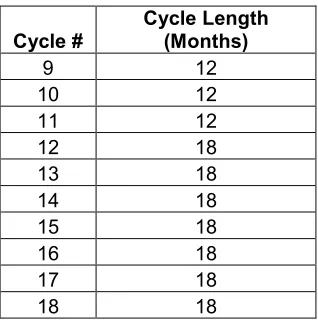
Unless noted otherwise, the cycle energy production schedule used for testing of relevant GA and parallel SA parameters is as presented in Table 2-1.

Table 2.1: Energy production schedule used

Cycle #

Cycle Length (Months)

9 12

10 12

11 12

12 18

13 18

14 18

15 18

16 18

17 18

18 18

2.1 Genetic Algorithms 2.1.1 Crossover Type

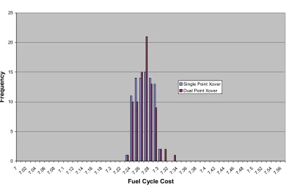
It is possible for crossover to be applied to multiple points. The mechanics of the operation are very similar. The only difference is that two or more crossover points are selected per set of strings. The theoretical reasoning behind multiple crossover points is that multiple crossover points allow a more uniform sharing of genes.

Crossover Type Comparison

0 5 10 15 20 25

7

7.02 7.04 7.06 7.08 7.1 7.12 7.14 7.16 7.18 7.2 7.22 7.24 7.26 7.28 7.3 7.32 7.34 7.36 7.38 7.4 7.42 7.44 7.46 7.48 7.5 7.52 7.54 7.56

Fuel Cycle Cost

F

re

q

u

e

n

c

y

Single Point Xover Dual Point Xover

Figure 2.1: Comparison of Crossover Types

Table 2.2: Comparison of Crossover Types

AVG STD

Single Point 7.2617 0.0171

Dual Point 7.2631 0.0185

2.1.2 Initial Population

The initial population of feed region size per cycle in the planning horizon is generated from an equilibrium cycles approximation. Maximum diversity is desired in genetic algorithms because it is analogous to widening the gene pool as much as possible so that it is possible, for the very best schemes to be bred

schemes which fall within the equilibrium cycles and a pre-defined range. It is important to note that this range must be a multiple of the symmetry constraint on feed region size.

Due to the way the matrix is defined, each cycle has the same number of possible sizes of fresh assemblies to be loaded. An example of such a matrix is the following.

Table 2.3 Example of Possible Feed Region Sizes

Cycle Possible Feed Region Sizes

5 40 44 48 52 56

6 52 56 60 64 68

7 52 56 60 64 68

In the above table, the left hand column shows the cycle number and the rows correspond to the possible feed region sizes for that cycle. OCEON-P chooses the relevant sizes by

randomly generating a number between one and the total number of cells left in that cycle. For example, for the above scheme, the first iteration would pick a random number between one and five, as there are five different possible feed region sizes for each cycle. The number that is picked is then used as the feed region size for that cycling scheme on that particular cycle. The next iteration around, the code would pick a number, i, between one and four. The code would then find the ith feed region size that is not already taken. This process continues until the initial population is filled. If all the options in the matrix are taken before the initial population is filled, the selection matrix is emptied and the process starts over at whichever member of the initial population filled the matrix. This method ensures that all feed region ‘genes’ are represented. The number of cycling schemes required to span the entire space is quite small so having too small a population size to have all possible schemes reachable by crossover is not a concern. For example, if the user defined band is set so that ten feed region sizes are possible then an initial population of ten is all that is required to completely span the space.

2.1.3 Soft Constraints in Genetic Algorithms

selection operator in genetic algorithms is mainly based on the fitness of the solution. Soft constraints, by adding the penalties on top of the true fuel cycle cost, create the type of fitness function that GAs demand.

With consideration to the usage of soft constraints, the fitness function of each string is simply the augmented fuel cycle cost and can then be written as

∑

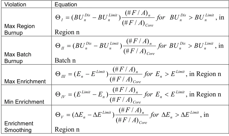
where F is the levelized fuel cycle cost. The lambda values denote penalty factor coefficients. The theta values are the penalty functions associated with the various OCEON-P violations. There are five such violations. The size of the violation is the absolute difference between the allowable limit and the value of the item being limited. The size of the violation is then weighted by the ratio of the number of violating assemblies and the total number of

assemblies. For example, violations involving batches will be multiplied by the ratio of the batch and the total number of assemblies. Therefore, the summation denoted in equation 2.1 extends over all constraints over all cycles, i.e. regions and batches in the planning horizon.

Table 2.4 OCEON-P Violation Types Violation Equation

Max Region Burnup for A F A F BU BU Core n Limit n Dis n I ) / (# ) / (# ) ( − = Θ Limit n Dis n BU

BU > , in Region n Max Batch Burnup for A F A F BU BU Core n Limit n Dis n II ) / (# ) / (# ) ( − = Θ Limit n Dis n BU

BU > , in Batch n Max Enrichment for A F A F E E Core n Limit n III ) / (# ) / (# ) ( − = Θ Limit n E

E > , in Region n

Min Enrichment for A F A F E E Core n n Limit IV ) / (# ) / (# ) ( − = Θ Limit n E

E < , in Region n

Enrichment Smoothing for A F A F E E Core n Limit n V ) / (# ) / (# ) (∆ −∆ = Θ Limit n E

E >∆

∆ , in

Similar to simulated annealing, as the search progresses the GA optimization is intended to cause any history with violations to become very expensive, decreasing the probability of selection in the genetic process. The lambda values are the means to this end by being a penalty factor coefficient that increases with each generation. Its purpose is to weight the relative importance of each penalty function as well as increasingly penalize the schemes with penalties as the search progresses. In utilizing the soft constraints, it is also necessary that the lambda multipliers are not too large at the beginning of the search because this would be detrimental to the diversity of the gene population by pushing the solution pool into a niche too early in the optimization. Therefore, we would like the lambda multipliers to be neither increased too quickly nor too slowly in the search. This is accomplished by

retaining a similar version of the lambda multiplier adaptation from simulated annealing in the GA. The difference is that the lambda multipliers are updated at each generational step instead of each cooling step.

The calculation of the values of lambda is based upon the three point iteration scheme. )

(

1 1 2

1 *( )

t k N L N k n k k k k k − − − − + Λ Λ Λ Λ = χ λ λ

λ (2.2)

In the above equation L is the length of the search, N_t is the total number of histories evaluated at the point of update, N_k is the number of histories evaluated in that particular update step, and Λ_k is the average size of a particular violation in the population for the particular update step. Chi and Λ_nare fixed for each penalty type. The lambda multipliers are initiated at the beginning of the search based upon the initial population by the expression

n n n n _σ σ λ λ

λ = ˆ ~ 0 _(2.3)

where the first two lambda values are constants, sigma naught corresponds to the standard

deviation of the objective function and sigma n is the standard deviation of the nth penalty

function.

An issue occurs, however, at high generational numbers when the lambda multipliers

the gene pool. These high violation schemes combined with the exacerbating effect of high lambda multipliers will create unreasonably high augmented fuel cycle costs that have a significant adverse effect on the gene pool. The solution to this problem is an adaptation of what was done in the previous version of the code which utilized simulated annealing, which was to stop the lambda multiplier updates after they had reached a certain magnitude. In GA, the lambda multiplier updates stop after a certain generation has been reached.

2.1.4 Selection

A commonly accepted means of selection is called ranking. This method involves ranking all schemes in the current gene pool from one to the number of schemes in the pool. This rank, k, is then used to create a probability distribution function which can take any number of forms. These forms are called scaling types. One of the simplest possibilities for scaling is the linear type, or

bk a

k]= +

Pr[ (2.4)

Power scaling is also possible. In this case the probability distribution for power two scaling

would be expressed as

2

]

Pr[k =a+bk (2.5)

In any sort of ranking scheme, the probability distribution has certain properties that

allow for the closed form solution of the constants a and b. Firstly, all probability

distributions must sum to one.

∑

=

=

N

k

k

1

1 ]

Pr[ (2.6)

Additionally, in order to control how likely a scheme of a particular rank will be selected, an

expression for population pressure is required. Using the definition presented by Reeves,

pressure is taken to be the probability of selecting the best string divided by the probability of

selecting the median string. The pressure can thus be presented as

2 ) 1

( +

+ + =

N b a

b a

φ (2.7)

4 ) 1 ( + 2

+ + =

N b a

b a

φ (2.8)

for power two ranking. Note that the above two definitions for pressure imply that the best string is represented when k is equal to one. Additionally, since typically the total number of fuel cycling schemes in each generation is even, the median in both linear and power two scaling is simply expressed as the population size divided by two.

Applying the restrictions imposed by equations 2.7 and 2.8 and utilizing certain summation equalities, the coefficients a and b for linear scaling are found to be

) 1 (

2

− + − =

N N

N

a φ φ ,

) 1 (

) 1 ( 2

− − =

N N

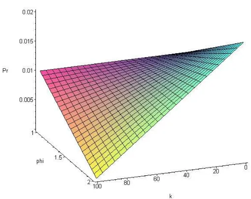
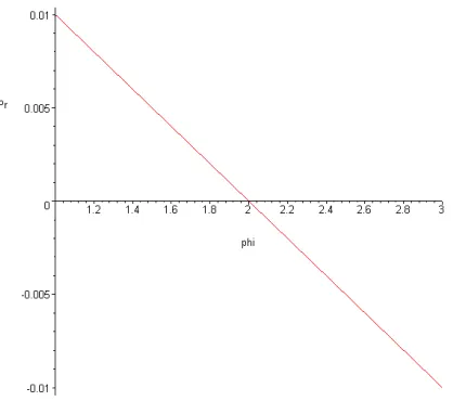
b φ (2.9) The resulting distribution looks like

It follows then that for linear scaling, the domain of the selection pressure is between one and two. This is because in the case of the 100th ranked scheme, any pressure greater than two would result in a non-physical negative selection probability.

Figure 2.3: First Order Domain Violation Range

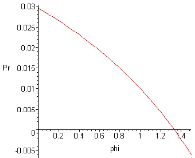
In a similar fashion, for power two scaling the coefficients are found to be

) 10 6 4 2 6 ( ) 4 ( 3 2 2 2 + − − + + − = N N N N N N a φ φ φ φ , ) 10 6 4 2 6 ( ) 1 ( 12 2

2 _{+ + − − +}

Figure 2.4: Second Order Probability Distribution

Similar to linear scaling, the power two scaling case also imposes restrictions on the domain of the pressure. In this case, pressure may go from one to 1.3 for the reason that anything beyond this value for the 100th ranked case would result in negative probabilities.

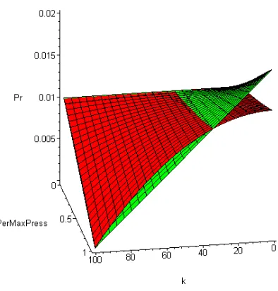
To keep things in perspective a graph comparing the two ranking schemes is presented. Since the two ranking schemes have different domains, the domain for the combined graph as presented below is the percentage of the maximum allowable pressure.

Figure 2.6: Scaling Domain Comparison

Both figures 2.2 and 2.4 have the properties that at maximum pressure phi, the probability of selecting the worst scheme (k=population size) is near zero; at minimum pressure, the entire spectrum of ranks have a similar chance to be selected.

Comparison of Linear and Second Order Scaling 0 5 10 15 20 25 30 7 7 .0 2 7 .0 4 7 .0 6 7 .0 8 7 .1 7 .1 2 7 .1 4 7 .1 6 7 .1 8 7 .2 7 .2 2 7 .2 4 7 .2 6 7 .2 8 7 .3 7 .3 2 7 .3 4 7 .3 6 7 .3 8 7 .4 7 .4 2 7 .4 4 7 .4 6 7 .4 8 7 .5 7 .5 2 7 .5 4 7 .5 6 7 .5 8 7 .6 7 .6 2 7 .6 4 7 .6 6 7 .6 8 7 .7

Best Augmented FCC in 6000 History Run

F re q u e n c y Linear Second Order

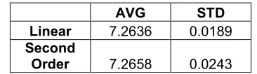
Figure 2.7: Scaling Type Result Comparison

Table 2.5: Scaling Type Result Comparison

AVG STD

Linear 7.2636 0.0189

Second

Order 7.2658 0.0243

2.1.5 Archiving and Elitism

he best solution found by the GA throughout the entire search. Two solutions are applied which attempt to solve this problem, elitism and archiving.

The idea behind elitism carryover is that the best cycling schemes from the previous generation should be implemented in the current generation so that their good genes are passed on. Care is taken with the elitism carryover not to re-run the case as it has been saved. Furthermore, the operations of GA (crossover, mutation) etc., are only applied after the best from the current generation is saved.

It is possible, however, since elitism deals with augmented fuel cycle costs, that the carried over schemes may contain violations. This is where the advantage of archiving becomes apparent. If the conditions for entrance into the archive are stringent enough, no violations will be present for the stored schemes. The two criterion used for entrance into the archive are no violations must be present and that the scheme to be archived must be less expensive than the most expensive scheme currently in the archive. The no violation requirement is difficult for GA to achieve in large quantities, as indicated in the lambda multiplier section. Table 2.5 indicates the effect of archiving.

Table 2.6: Archiving Implementation

Archive No-Archive Difference

7.286699 7.29244 0.00575 7.279001 7.27900 0 7.270708 7.27609 0.00538 7.26642 7.26642 0 7.286699 7.29244 0.00575

2.1.6 Probability Distributions for Feed Size Selection

Mutation in GA is biased by the probability distribution functions that were

assemblies was at the edge of the distribution. An example to illustrate this point is the following. Suppose the minimum and maximum assemblies for a particular cycle are 40 and 100. The distribution is reset to 36 and 104 if there was a scheme that called for 40 new assemblies in that particular cycle.

This method is not acceptable in the GA method of optimization because at high mutation rates, it is highly probable that this increase in scope will go beyond the range of the array. This in turn causes severe problems with the code. The solution to this problem

involved only expanding the distribution range if it became smaller than the bands placed around the equilibrium cycle approximation used to generate the initial population.

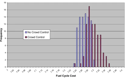
2.1.7 Crowding and Niching

It has been proposed in the field of GAs that having too many genes with similar characteristics in the gene pool is undesirable. The theory is that these genes create a niche that only cuts down on the diversity of the population on a whole. A common distance keeping scheme is based upon the sharing function proposed by Goldberg and Richardson. [15]

Each cycling scheme has a distance from every other cycling scheme. This distance is taken to be the root mean square difference of two schemes. For example, the distance

between cycling schemes

[

]

a= , , ,

[

]

b= , , , would be

(

)

n g m f l e k d d_ij

2

2 2

2 2

2

) ( ) ( ) ( )

( − + − + − + −

= (2.12)

where the denominator is the maximum distance that two schemes can be apart, which is

twice the maximum range between region sizes defined by the user multiplied by the number

of total schemes in the planning horizon. Since we define two schemes being too close to

D d

h_ij =1− ij if d_ij <D,

0

=

ij

h if d_ij >D (2.13)

where the value D gives the user additional control to increase or decrease the severity of the

anti-grouping function. Finally,

∑∑

= −

=

= N

i i

j ij

h Q

1 1

1

(2.14)

is the crowding factor.

It is easy to see that, due to the nature of its derivation, Q will be bigger in schemes which are

closer to other schemes (because

D d_ij

would be smaller if d_ij is small, or the schemes are

‘close’). Therefore, if we multiply the augmented fuel cycle cost by the scaling factor, we

have effectively made less likely that the schemes that are closer to other schemes will be

selected to breed.

The disadvantage, however, of crowd control is that by breaking up crowds of similar

cycling schemes, one may be breaking up groups of good genes. In this argument lies the

crux of the niching theory, and any optimization scheme. In most real world problems it is

impossible to know which crowds are around the true minimum and which crowds are just

local minima. The presented data was generated by executing OCEON-P one hundred times

using different random seeds, with the composite results used to determine the average

Crowd Control Function Effects

0 2 4 6 8 10 12 14 16 18

7

7.02 7.04 7.06 7.08 7.1 7.12 7.14 7.16 7.18 7.2 7.22 7.24 7.26 7.28 7.3 7.32 7.34 7.36 7.38 7.4

Fuel Cycle Cost

F

re

q

u

e

n

c

y

No Crowd Control

Crowd Control

Figure 2.8: Niche Control Implementation

Table 2.7: Niche Control Implementation

AVG STD

CC 7.289011 0.022927

No CC 7.261716 0.017142

The tables and figures above show that the application of this particular niching scheme in OCEON-P yields undesirable cycling schemes. The most likely explanation is that the crowding scheme is breaking up groups of similar cycling schemes which contain

favorable solutions.

2.1.8 Tuning Parameter Optimization

gives a general idea of the regimes in which certain common parameters should reside. However, in order to obtain a more narrow set of parameters in the specific context of the OCEON-P computer code, it is necessary to perform tests to find the optimum set of GA tuning parameters.

The test performed involved generating sets of tuning parameters which were allowed to vary within the ranges prescribed by literature. In other words, each tuning parameter within each set is randomly generated within a certain domain. Each set was then repeated multiple times using a different random number seed to obtain the average levilized fuel cycle cost for feasible schemes and the associated standard deviation.

Population Size

7.26 7.27 7.28 7.29 7.3 7.31 7.32

50 55 60 65 70 75 80 85 90 95 100

Population Size

A

v

e

ra

g

e

N

o

V

io

la

ti

o

n

F

u

e

l

C

y

c

le

C

o

s

t

FCC Standard Deviation with Population Size Variation 0 0.005 0.01 0.015 0.02 0.025 0.03 0.035 0.04 0.045

50 55 60 65 70 75 80 85 90 95 100

Population Size S ta n d a rd D e v ia ti o n

Figure 2.10: FCC standard deviations with changing population sizes

Crossover 7.26 7.27 7.28 7.29 7.3 7.31 7.32

0.7 0.75 0.8 0.85 0.9 0.95 1

Probability of Crossover

A v e ra g e N o V io la ti o n F u e l C y c le C o s t

Standard Deviations for Varying Crossover Probability 0 0.005 0.01 0.015 0.02 0.025 0.03 0.035 0.04 0.045

0.7 0.75 0.8 0.85 0.9 0.95 1

Crossover Probability S ta n d a rd D e v ia ti o n

Figure 2.12: FCC standard deviations with changing crossover probability

Mutation 7.26 7.27 7.28 7.29 7.3 7.31 7.32

0.01 0.06 0.11 0.16 0.21 0.26 0.31

Probability of Mutation

A v e ra g e N o V io la ti o n F u e l C y c le C o s t

FCC Standard Deviations with Mutation Variation 0 0.005 0.01 0.015 0.02 0.025 0.03 0.035 0.04 0.045

0.01 0.06 0.11 0.16 0.21 0.26 0.31

Mutation Chance S ta n d a rd D e v ia ti o n

Figure 2.14: FCC standard deviation with mutation probability variation

Pressure 7.26 7.265 7.27 7.275 7.28 7.285 7.29 7.295 7.3 7.305 7.31

1.5 1.55 1.6 1.65 1.7 1.75 1.8 1.85 1.9 1.95 2

Pressure A v e ra g e N o V io la ti o n F u e l C y c le C o s t

FCC Standard Deviation with Pressure Variation 0 0.01 0.02 0.03 0.04 0.05 0.06

1.5 1.55 1.6 1.65 1.7 1.75 1.8 1.85 1.9 1.95 2

Pressure S ta n d a rd D e v ia ti o n

Figure 2.16: FCC standard deviation with variation in pressure

% Carried From Previous Generation

7.26 7.27 7.28 7.29 7.3 7.31 7.32

0 0.05 0.1 0.15 0.2 0.25 0.3 0.35 0.4

% Carried A v e ra g e N o V io la ti o n F u e l C y c le C o s t

FCC Standard Deviation with % Carried From Previous Generation Variation

0 0.005 0.01 0.015 0.02 0.025 0.03 0.035 0.04 0.045

0 0.05 0.1 0.15 0.2 0.25 0.3 0.35 0.4

% Carried

S

ta

n

d

a

rd

D

e

v

ia

ti

o

n

Figure 2.18: FCC standard deviation with elitism percentage variation

When examining the results presented in the figure, what is desired are parameter values that produce low fuel cycle costs in combination with low standard deviations.

Generally, the sensitivity analysis of the GA tuning parameters in OCEON-P agreed with the values prescribed by the literature. High standard deviations are prevalent, however, because of the randomness of selecting the parameter sets. That is to say, it was possible for an optimal and non-optimal parameter values to be paired together. Without knowing how tuning parameters affect each other exactly, however, it would have been unfair to perform the test in another manner. The effect of other parameters can be seen in the figures if more than one result is shown for a fixed value of the parameter being presented in the figure, i.e. the x axis.

Results for the crossover optimization of the OCEON code generally confirm the empirical and theoretical assertion from the literature that high crossover probabilities generally lead to superior results.

Mutation variations in the OCEON code also have a predictable effect on the fuel cycle costs; that is, lower mutation probabilities generally causes a more favorable result. It is also worth noting that lower mutation probabilities result in a more robust solution. This is not surprising because lower mutation implies that less variation is introduced to the gene pools over the course of the optimization.

The above figures also show that the highest selection pressure is desirable in finding the lowest fuel cycling scheme. This implies that although a high selection pressure will have the effect of decreasing the diversity of the gene pool by continually selecting the best

schemes, the positive effect of pushing the gene pool towards the more feasible schemes dominates.

The tests imply an advantage to the inclusion of the elitism parameter. Generally, elitism rates of over twenty percent are undesirable. Standard deviations on the fuel cycle costs also generally increase after a twenty percent carry rate. This result generally agrees with the literature.

2.2 Parallel Simulated Annealing 2.2.1 Exchange of Information

Exchange of information in the parallel simulated annealing case begins with a certain number of acceptances having occurred across all processors. The processors then ‘fan in’ and send information about their archived solutions to a central processor. This central processor then sorts through the solutions from all processors and pulls out the best cycling schemes while ignoring duplicates to fill the new archive that all the processors will start from at the beginning of the new update step. In this manner, the probability

The new temperature and lambda multipliers to be used in the next cooling step are based upon statistics generated across all processors.

In the non-parallel case, the temperature was updated according to

T_k+1 =αT_k (2.15) where

) exp(

f k

T

σ ν

α = − (2.16)

Nu is a constant and sigma is the standard deviation of the objective function. The initial cooling step is used to gather statistics required to tabulate initial penalty multipliers and initial temperature. As such, there are no rejections in the initial cooling step. The initial temperature is calculated as

T = Aσ_f (2.17) where A is also a constant. This temperature is then used to calculate acceptance

probabilities in the next cooling step. In the parallel case, the difference is that the sigma values now correspond to the objective function standard deviations of all histories examined up until the end of the initial cooling step from all the parallel processors. It follows,

therefore, that the values of T in the above equations would then refer to the temperatures used by all processors.

The values for lambda multipliers are also updated to use the information obtained from all processors. The three point iteration scheme (Equation 2.2) is still the basis of the calculations. The difference is that now the variables refer to a global value. For

exampleN_twould now correspond to the total number of histories evaluated across all processors. Similarly, the gamma values would refer to the average size of a certain violation when all histories from all processors are considered. Similarly, the values within the

expression for the initial value of the lambda multipliers

n n n

n _σ

σ λ λ

λ ₌ ˆ ~ 0 _(2.18)

2.2.2 MPI Overhead

The major source of overhead in the case of MPI implementation is the time required to pass information between processors. Message passing time is primarily a function of the size of the message. Work performed at the Sandia National Laboratories by Ron Brightwell and Douglas Doerfler (12) using different programs which resolve send and receive latency have shed light on this relationship. Figure 2.17 and 2.18 display their measured latency on different computer platforms. Considerable variations in latency as a function of processor numbers used is noted with computer platform.

Figure 2.20: MPI receive latencies

Another less significant source of overhead in the MPI implementation is that the fan in cannot proceed until every processor is at the fan in portion of the program. This means that at the end of each cooling step, one must wait at most the length of time required by the core simulator to go through a complete planning horizon. It is possible to calculate this wait time on an average basis using statistical methods. If one assumes that the amount of time required for each processor to reach the beginning of the fan in step to be uniformly and randomly distributed and we are interested in the maximum amount of time then we can write the cumulative probability distribution as

) ) ,...,

(max(x₁ x y

P _n ≤ , x₁,...,x_n ~unif[0,1]

The zero to one can be thought of as zero to one hundred percent of the time the core simulator requires to burn a full planning horizon. The cumulative probability function can further be written as

∏

=

≤ =

≤

≤ n

i i

n y P x y

x y x P

1

1 ,..., ) ( )

Since it is assumed that the x values are of a uniform distribution n n i n i

i y y y

x P

∏

∏

Turning a cumulative distribution density into a probability distribution density involves

taking a derivative which results in a probability distribution density of

1

−

= ∂

∂ n _n

ny y y

To find the expectation value of the probability distribution function we multiply by y and

integrate from zero to one.

∫

E _n n

Since n is the number of processors and there would be no wait time if one processor was

used, the average wait time can then be expressed as

n n−1

Therefore, assuming an average number of cooling steps and knowing the size of the

information that must be sent in each cooling step a model (figure 2.19) is constructed which

estimates the progression of efficiency as the number of processors is increased. The

experimental data presented in the below figure are based upon runs with ten random seeds

and the indicated number of processors. Time required to traverse seven thousand histories

was recorded and the corresponding efficiencies and standard deviations were calculated.

Theoretical and experimental values use an average of two seconds for every cycling scheme

depletion, and display good agreement. To generate the theoretical efficiency, the total

number of sends and receives along with the relevant latencies were tabulated for multiple

numbers of processors. With consideration given to this and the overhead associated with

wait times at each fan in step, the expected decrease in run time as a function of number of

processors used was calculated. The quality of the solutions found as a function of the

MPI Overhead

0 0.2 0.4 0.6 0.8 1 1.2 1.4

0 1 2 3 4 5 6 7 8 9 10 11 12 13 14 15 16 17 18 19 20

# Processors

E

ff

ic

ie

n

c

y

Experiment Theory

Figure 2.21: MPI overhead

3 Results

3.1 Genetic Algorithms Results

Parameters suggested by the literature were used to compare the genetic algorithm search against the single processor simulated annealing search. The tuning parameters used in the genetic algorithm are given in Table 3.1

Table 3.1: Parameters used for final GA study

Cross 100%

Mutate 10%

Gen Size 100

Histories 6000

Six thousand histories were run for the simulated annealing and genetic algorithm cases. The results are presented in the form of a histogram. Each optimization method was run 795 times with as many random seeds. The best feasible schemes found, using only the LRM core simulator, are used to generate Figure 3.1, which presented the frequency of obtaining a fuel cycle cost over a certain range.

0 10 20 30 40 50 60 70 80

7.2 7.21 7.22 7.23 7.24 7.25 7.26 7.27 7.28 7.29 7.3 7.31 7.32 7.33 7.34

FCC Bin

F

re

q

u

e

n

c

y

GA

SA

Figure 3.1: GA and SA comparison of best solution found

Table 3.2: GA and SA comparison of best solution found

MEAN MEDIAN STD

SA 7.25336 7.25131 0.015688

GA 7.25705 7.25582 0.018618

The results show that the current implementation of GA and SA are very similar in both robustness and economy of fuel cycle cost when it comes to the best solution found.

SA

7.16 7.21 7.26 7.31 7.36 7.41 7.46

1 2 3 4 5 6 7 8 9 10 11 12 13 14 15 16 17 18 19 20 21 22 23 24 25 26 27 28 29

Seed #

F

u

e

l

C

y

c

le

C

o

s

t

min max avg

Figure 3.2: SA overall performance

GA

7.16 7.21 7.26 7.31 7.36 7.41 7.46

1 2 3 4 5 6 7 8 9 10 11 12 13 14 15 16 17 18 19 20 21 22 23 24 25 26 27 28 29

History #

F

u

e

l

C

y

c

le

C

o

s

t

min max avg

The above figures show the behavior of acceptable solutions in the final archive in the cases of simulated annealing and genetic algorithms. As shown previously, the minimum values of fuel cycle cost for each case are very comparable. However, due to the disruptive nature of genetic algorithms, a larger spread of solutions is found, resulting in a higher average FCC. This point is further illustrated by the convergence behavior of the two optimization methods as shown below.

GA and SA Convergence

7.27 7.28 7.29 7.3 7.31 7.32 7.33 7.34

0 1000 2000 3000 4000 5000 6000 7000

History

A

v

e

ra

g

e

N

o

V

io

la

ti

o

n

F

C

C

GA SA

Figure 3.4: GA and SA convergence behavior

3.2 Parallel Simulated Annealing Results

In the implementation of parallel simulated annealing, the primary interest is how the method scales with the introduction of multiple processors. This information is presented in Figure 3.5.

To generate the figure, average fuel cycle costs for all feasible schemes found per cooling step were recorded as a function of history and number of processors utilized in the run. This was done for ten random seeds on each number of processors.

Cell Averaged FCC Cost

7.21 7.22 7.23 7.24 7.25 7.26 7.27 7.28 7.29 7.3

0 2000 4000 6000 8000 10000 12000 14000

History

A

v

e

ra

g

e

F

C

C

1 Processor 4 Processors 8 Processors 12 Processors 16 Processors

Figure 3.5: Parallel simulated annealing performance

4 Conclusions and Future Work 4.1 Conclusions

The implementation of parallel simulated annealing into the OCEON-P algorithm resulted in a significant decrease in run times without a decrease in the quality or robustness of the solutions. This result generally agrees with other out-of-core optimization studies in the field (16). The fact that quality and robustness remain consistent up to sixteen processors utilized may imply that shorter Markov chains associated with the simulated annealing in each individual processor is not detrimental to the search progression. These favorable results may also be facilitated by the exchange of information which occurs at each fan in step along the way. One must note, however, that because of the overhead associated with the usage of the message passing interface, the amount of time saved with each incremental processor does not proceed in a linear manner. In fact, efficiency drops to just over sixty percent with twenty processors used.

The implementation of genetic algorithms to the OCEON-P code resulted in less desirable results when compared to what simulated annealing could accomplish. Research was performed on the various tuning parameters and options available for the genetic algorithm method. These include crossover type, selection type, the presence of crowding functions, and appropriate values for crossover, pressure, mutation, elitism and population size. After this investigation however, it was concluded that although genetic algorithms could locate the same caliber of best solutions for a given planning horizon, simulated

annealing could locate a better family of acceptable solutions. The highly disruptive nature of the genetic algorithm search along with the large amount of significant tunable parameters and options may contribute to the method’s non-suitability for this specific out-of-core nuclear fuel optimization problem.

4.2 Recommendations for Future Work

rotation templates available. Without acceptable templates, it is impossible for the

optimization to find the global minimum because the minimum would not exist in the search space. To date, the same set of templates is used for every planning horizon and no suitable system for generating new templates exists. Additionally, although parallel simulated

annealing has replaced conventional serial simulated annealing as the optimization engine in the version of OCEON-P which uses SIMULATE-3, SIMULATE-3 and OCEON-P remain separate programs and must communicate with each other via input and output decks created in the intermittent steps of the optimization. The use of MPI may be extended to more

References

[1] D.E. Goldberg and R. Lingle. “Alleles, loci and the traveling salesman problem”. In J.J. Grefenstette (Ed.) “Proceedings on an International Conference on

Genetic Algorithms and Their Applications”. Lawrence Erlbaum Associates, Hillsdale, New Jersey, 154-159. 1985

[2] J.J. Grefenstette. “Optimization of control parameters for genetic algorithms”. IEEE-SMC, SMC-16. 1986

[3] D.E. Goldberg, K.Deb and J.H. Clark. “Genetic algorithms, noise, and the sizing of populations”. Complex Systems, 6, 333-362. 1992

[4] C.R. Reeves (Ed.). “Modern Heuristic Techniques for Combinatorial Problems”. Blackwell Scientific Publications, Oxford, UK. 1992.

[5] K. A. DeJong, “Genetic algorithms: A 10 year perspective”. Proceedings of an International Conference of Genetic Algorithms and theirApplications.

(J. Greffenstette, editor), Pittsburgh, pp. 169-177. 1985

[6] J. D. Schaffer et. al., “A study of control parameters affecting online performance of genetic algorithms for function optimization”. Proceedings of the Third International Conference on Genetic Algorithms,pp. 51-60. 1989

[7] I. M. Oliver, D. J. Smith and J. R. C. Holland. “A study of permutation crossover operators on the travelling salesman problem”. Proceedings of the Second

International Conference of Genetic Algorithms, pp. 224-230. 1987

[8] Reeves, Colin R and Jonathan E. Rowe. “Genetic Algorithms-Principles and Perspectives”. Kluwer Academic Publishers. 2003

[9] Goldberg, David E. “Genetic Algorithms in Search, Optimization and Machine Learning”. Addison-Wesley Publishing Company, Inc. 1989

[10] K Deb and A Pratap et al. “A fast and Elitist multiobjective genetic algorithm”. IEEE transactions on Evolutionary computation, Vol 6 No. 2002

[11] E. Zitzler and L. Thiele. “Multiobjective optimization using evolutionary

[12] Brightwell, Ron and Douglas Doerfler. “Measuring MPI Send and Receive

Overhead and Application Availability in High Performance Network Interfaces”. Center for Computation, Computers, Information and Math. Sandia National Laboratories. 2006.

[13] OCEON-P Version 2.0.0 Users Manual. Electric Power Research Center, North Carolina State University, Raleigh (1998).

[14] Anderson, Kenneth A. “Implementation of Soft Constraints and

Simulated Annealing Algorithm in OCEON-P and Linkage of OCEON-P and SIMULATE3”. North Carolina State University. 2007

[15] D.E. Goldberg and J. Richardson. “Genetic algorithms with sharing for multimodal function optimization”. In J.J. Grefenstette (Ed.) Proceedings of the 2nd International Conference on Genetic Algorithms. Lawrence Erlbaum Associates, Hillsdale, NJ, 41-49. 1987