Using Simulated Annealing and Ant-Colony
Optimization Algorithms to Solve the
Scheduling Problem
Nader Chmait
,
Khalil Challita
∗Department of Computer Sciences, Faculty of Natural and Applied Sciences, Notre-Dame University, Louaize, Zouk Mosbeh, Lebanon
∗Corresponding author: [email protected]
Copyright c⃝2013 Horizon Research Publishing All rights reserved.
Abstract
The scheduling problem is one of the most challenging problems faced in many different areas of everyday life. This problem can be formulated as a combinatorial optimization problem, and it has been solved with various methods using meta-heuristics and intelligent algorithms. We present in this paper a solution to the scheduling problem using two different heuristics namely Simulated Annealing and Ant Colony Optimization. A study comparing the performances of both solutions is described and the results are analyzed.Keywords
ACO, Ant Colony Optimization, SA, Simulated Annealing, Scheduling Problem, Exam Scheduling, Timetabling1
Introduction
A wide variety of scheduling (timetabling) problems have been described in the literature of computer science during the last decade. Some of these problems are: the weekly course scheduling done at schools and universities[1], examination timetables[2], airline crew and flight scheduling problems[3], job and machine scheduling[4], train (rail) timetabling problems[5] and many others. . .
Many definitions of the scheduling problem exist. A general definition was given by A. Wren[6] in1996 as: “The allocation of, subjects to constraints, of given resources to objects being placed in space and time, in such a way as to satisfy as nearly as possible a set of desirable objectives”.
Cook[7] proved the timetabling problem to be NP-complete in1971, then Karp[8] showed in1972 that the general problem of constructing a schedule for a set of partially ordered tasks among k -processors (where k is a variable) is NP-complete. Four years later, a proof[9] showing that even a further restriction on the timetabling problem (e.g the restricted timetable problem) will always lead to an NP-complete problem. This means that the running time for any algorithms currently known to guarantee an optimal solution is an exponential function of the size of the problem. The complexity results of the some of the scheduling problems were classified and simulated in[10] and their reduction graphs were plotted.
The exam scheduling is still done manually in most universities, using solutions from previous years and altering them in such a way to meet the present constraints related to the number of students attending the upcoming exams, the number of exams to be scheduled, the rooms and time available for the examination period. We propose an improved methodology where the generation of the examination schedules is feasible, automated, faster and less error prone.
Even though we present in this paper our solution in the context of the exam scheduling problem, we can generalize it to solve many different scheduling problems with some minor modifications regarding the variables related the the problem in hand and the resources available.
An informal definition of theexam scheduling problem is the following:
The main hard constraints[12] are given below:
1. No student is scheduled to sit for more thanoneexam simultaneously. So any two exams having students in common should not be scheduled in the same period.
2. An exam must be assigned to exactly oneperiod.
3. Room capacities must not be violated. So no exam could take place in a room that has not a sufficient number of seats.
As for the soft constraints, they vary between different academic institutions and depend on their internal rules[13]. The most common soft constraints are:
1. Minimize the total examination period or, more commonly, fit all exams within a shorter time period. 2. Increase students’ comfort by spacing the exams fairly and evenly across the whole group of students. It is
preferable for students not to sit for exams occurring in two consecutive periods.
3. Schedule the exams in specific order, such as scheduling the maths and sciences related exams in the morning time.
4. Allocate each exam to a suitable room. Lab exams for example, should be held in the corresponding labs. 5. Some exams should be scheduled in the same time.
We will attempt to satisfy all the hard-constraints listed above. Regarding the soft-constraints, we will address the first two points, whereby we try to enforce the following:
1. Shorten the examination period as much as possible
2. A student has no more thanoneexam intwoconsecutive time-slots of the same day.
In other words, we will try to create an examination schedule spread among the shortest period of time and therefore use the minimum number of days to schedule all the exams, we also spread the exams shared by students among the exam schedule in such a way that they are not scheduled in consecutive time-slots.
This paper is organized as follows. Section 2 presents the mathematical formulation of the exam scheduling problem; Section 3 describes the main structures of the SA (Simulated Annealing) and ACO (Ant Colony Opti-mization) algorithms. We list and describe in Section 4 some of the heuristics and algorithms that are used in solving the scheduling problem. In Section 5 and 6 we present and discuss our own approach to solving the exam scheduling problem using the Simulated Annealing and Ant Colony Optimization algorithms respectively and the empirical results of both solutions are shown in Section 7. Section 8 is a performance analysis and a comparative study between the two solutions. Finally we give a brief conclusion.
2
The Scheduling Problem
2.1
Problem FormulationWe will use a variation of D. de Werra’s[14] definition of the timetabling problem. Note that a class consists of a set of students who follow exactly the same program. So Let:
• C={c1,. . . ,cn}be a set of classes
• E={e1,. . . ,en}a set of exams
• S={s1,. . . ,sm}the set of students
• R={r1,. . . ,rx}the set of rooms available
• D={d1,. . . ,dz} the set of the examination days
• P={p1,. . . ,ps}the set of periods (sessions) of the examination days.
Since all the students registered in a class ci follow the same program, we can therefore associate for each class cian exam ei to be included in the examination schedule. So all the students registered in class ci will be required to pass the exam ei.
We will use the notation below:
•
espijk =
{
•
scji=
{
1, if student sjis taking class ci 0, otherwise
•
seji=
{
1, if student sjhas exam ei 0, otherwise
•
epiu=
{
1, if exam eiis held in period pu 0, otherwise
•
capacityzi=
{
number of seats in room rz, if rzholds ei
null, otherwise
We shall assume that all exam sessions have the same duration (say one period of two hours). We recap that the problem is, given a set of periods, we need to assign each exam to some period in such a way that no student has more thanoneexam at the same time, and the room capacity is not breached. We therefore have to make sure that the equations (constraints) below are always satisfied[14]:
1.
if capacityzi̸=null,∀sj∈S: m
∑
j=1
seji≤capacityzi (1)
2.
∀sj∈S,∀ei∈E, and onepk ∈: m
∑
j=1
espijk ≤1 (2)
3.
∀ei∈E,∀pu∈P: s
∑
u=1
epiu=|R| (3) *where|R| is equal to the number of rooms allocated for exams duringpu.
4.
∀cj ∈C∃ei∈E,pu∈P :epiu = 1 (4)
These equations reveal only the hard constraints which are critical for reaching a correct schedule. They must always evaluate to true otherwise we will end up by an erroneous schedule. We aim to find a schedule that meets all the hard constraints and try to adhere as much as possible to the soft constraints.
3
Heuristics And Optimization Algorithms
3.1
Simulated AnnealingThe idea behind simulate annealing (SA) comes from a physical process known as annealing[15]. Annealing happens when you heat a solid past its melting point and then cool it. If we cool the liquid slowly enough, large crystals will be formed, on the other hand, if the liquid is cooled quickly the crystals will contain imperfections. The cooling process[16] works by gradually dropping the temperature of the system until it converges to a steady, frozen state. SA exploits this analogy with physical systems in order to solve combinatorial optimization problems. We define S to be the solution space, which is the finite set of all available solutions of our problem, and f as the real valued cost function defined on members of S. The problem[17] is to find a solution or state,i∈ S, which minimizes f over S. SA is a type of local search algorithm that starts with an initial solution usually chosen at random and generates a neighbour of this solution, and then the change in the costf is calculated. If a reduction in cost is found, the current solution is replaced by the generated neighbour. Otherwise (unlike local search and descent algorithms, like thehill climbing algorithm), if we have an uphill move that leads to an increase in the value off, which means that, if a worse solution is found, the move is accepted or rejected depending on a sequence of random numbers, but with a controlled probability. This is done so that the system does not get trapped in what is called a local minimum[18] (as opposed to the global minimum where the near optimal solution is found). The probability of accepting a move which causes an increase inf is called the acceptance function and is normally set to:
whereT is a control parameter which corresponds to the temperature in the analogy with physical annealing[17]. We can see from (5) that, as the temperature of the system decreases, the probability of accepting a worse move is decreased, and when the temperature reacheszerothen only better moves will be accepted which makes simulated annealing act like a hill climbing algorithm[16] at this stage. Hence, to avoid being prematurely trapped in a local minimum, SA is started with a relatively high value ofT. The algorithm proceeds by attempting a certain number of neighborhood moves at each temperature, while the temperature parameter is gradually dropped. Algorithm 1 shows the SA algorithm as listed in [17].
Algorithm 1Simulated Annealing Algorithm
Select an initial solution i∈ S Select an initial temperature T0 >0
Select a temperature reduction functionα
Repeat
Set repetition counter n = 0
Repeat
Generate state j, a neighbor of i calculateφ = f(j) - f(i)
If φ < 0Theni := j
Else
generate random number x ∈]0,1[
If x<exp(-φ/t)Theni := j
n := n + 1
Untiln = maximum neighborhood moves
allowed at each temperature endif
endif
update temperature decrease function α
T =α·(T)
Untilstopping condition = true.
There are many important concepts in SA which are crucial for building efficient solutions. Some of these concepts are listed below:
• Initial Temperature
• Equilibrium State
• Cooling Schedule
• Stopping Condition
There are many ways in which these parameters are set, and they are highly dependent on the problem in hand and the quality of the final solution we aim to reach.
3.2
Ant Colony Optimization AlgorithmThe second algorithm (ACO) is a meta-heuristic method proposed by Marco Dorigo[19] in 1992 in his PhD thesis about optimization, learning and natural algorithms. It is used for solving computational problems where these problems can be reduced to finding good paths through graphs. The ant colony algorithms are inspired by the behavior of natural ant colonies whereby ants solve their problems by multi-agent cooperation using indirect communication through modifications in the environment via distribution and dynamic change of information (by depositing pheromone trails). The weight of these trails reflects the collective search experience exploited by the ants in their attempts to solve a given problem instance[20]. Many problems were successfully solved by ACO, such as the problem of satisfiability, the scheduling problem[21], the traveling salesman problem[22], the frequency assignment problem (FAP)[23]. . .
be performed by single ants, such as the invocation of a local optimization procedure, or the update of global information to be used to decide whether to bias the search process from a non-local perspective”[25].
The pseudo-code[26] for the ACO is shown below:
Algorithm 2Ant Colony Optimization Algorithm
Set parameters, Initialize pheromone trails
whiletermination condition not met do
ConstructAntSolutions ApplyLocalSearch (optional)
UpdatePheromones end while
3.2.1 Combinatorial Optimization Problem
Before going into the details of ACO, we will define a model[26] P = (S,Ω, f) of a combinatorial optimization problem (COP). The model consists of the following:
• a search spaceS defined over a finite set of discrete decision variablesXi:i= 1, . . . , n;
• a set Ω of constraints among the variables;
• an objective functionf :S→Rto be minimized. The generic variable Xi takes values v
j
i ∈ Di = {v1i, . . . , v| Di|
i }. “A feasible solution s ∈ S is a complete assignment of values to variables that satisfies all constraints in Ω”[26].
3.2.2 The Pheromone Model
We will use the model of the COP described in Subsection 3.2.1 above to derive the pheromone model used in ACO[27]. In order to do this we have to go through the following steps:
1. We first instantiate a decision variable Xi = v j
i (e.g a variable Xi with a value v j
i assigned from its domain Di)
2. We denote this variable by cij and we call it a solution component 3. We denote byC The set of all possible solution components.
4. Then we associate with each component cij a pheromone trail parameter Tij
5. We denote byτij the value of a pheromone trail parameter Tij and we call it the pheromone value 6. This pheromone value is updated later by the ACO algorithm, during and after the search iterations.
These values of the pheromone trails will allow us to model the probability distribution of the components of the solution.
The pheromone model of an ACO algorithm is closely related to the model of a combinatorial optimization prob-lem. Each possiblesolution component, or in other words each possible assignment of a value to a variable defines a pheromone value[26]. As described above, the pheromone valueτij is associated with the solution component
cij, which consists of the assignmentXi=v j i.
ACO uses artificial ants to build a solution to a COP by traversing a fully connected graphGC(V, E) called the
construction graph[26]. This graph is obtained from the set of solution components either by representing these components by the set ofvertices Vof Gc or by the set of itsedges E.
The artificial ants move from vertex to vertex along the edges of the graph GC(V, E), incrementally building a partial solution while they deposit a certain amount of pheromone on the components, that is, either on the vertices or on the edges that they traverse.
The amount ∆τ of pheromone that ants deposit on the components depends on the quality of the solution found. In subsequent iterations, the ants follow the path with high amounts of pheromone as an indicator to promising regions of the search space[26].
To model the ants’ behaviour formally, we consider a finite set of available solution componentsC={cij}, i=
set C[27]. We start from an empty partial solution sp =∅ and extend it by adding a feasible solutionsp using the components from the setN(sp)⊆C (where N(sp) denotes the set of components that can be added to the current partial solutionspwithout violating any of the constraints in Ω). It is clear that the process of constructing solutions can be regarded as a walk through the construction graphGC = (V, E).
The choice of a solution component fromN(sp) is done probabilistically at each construction step. Before describing the rules controlling the probabilistic choice of the solution components, we next describe an experiment that was run on real ants which derived these probabilistic choices, called the double-bridge experiment .
3.2.3 The Double-Bridge Experiment
In the double-bridge experiment, we have two bridges connecting the food source to the nest, one of which is significantly longer than the other. The ants choosing by chance the shorter bridge are of course, the first to reach the nest[27]. Therefore, the short bridge receives pheromone earlier than the long one. This increases the probability that further ants select it rather than the long one due to the higher pheromone concentrations over it (Fig. 1). FORAGING AREA NEST 00 00 11 11 00 00 00 11 11 11 0 0 1 1 0 0 0 1 1 1 00 00 11 11 0 0 0 1 1 1 0 0 1 1 00 00 00 11 11 11 FORAGING AREA NEST 00 00 00 11 11 11 0 0 0 1 1 1 00 00 11 11 00 00 11 11 00 00 00 11 11 11 00 00 11 11 00 00 00 11 11 11 00 00 11 11 00 00 00 11 11 11 00 00 00 11 11 11 00 00 11 11 00 00 00 11 11 11 00 00 00 11 11 11 0 0 1 1 0 0 0 1 1 1 00 00 00 11 11 11 00 00 11 11 00 00 00 11 11 11 0 0 0 1 1 1 00 00 11 11 00 00 11 11 00 00 00 11 11 11 00 00 00 11 11 11 0 0 1 1 00 00 11 11 00 00 11 11 0 0 1 1 00 00 11 11 0 0 1 1 00000000000000 00000000000000 00000000000000 0 0 11111111111111 11111111111111 11111111111111 11111111111111 11111111111111 00 00 00 00 00 11 11 11 11 11 00000000000000 11111111111111 0 0 0 0 0 0 0 0 0 0 0 0 0 0 0 0 0 0 0 0 0 0 0 0 0 0 0 0 0 0 0 0 0 0 0 0 0 0 0 0 0 1 1 1 1 1 1 1 1 1 1 1 1 1 1 1 1 1 1 1 1 1 1 1 1 1 1 1 1 1 1 1 1 1 1 1 1 1 1 1 1 1 0 0 0 0 0 0 0 0 0 0 0 0 0 0 0 0 0 0 0 0 0 0 0 0 0 0 0 0 0 0 0 0 0 0 0 0 0 0 0 0 0 0 1 1 1 1 1 1 1 1 1 1 1 1 1 1 1 1 1 1 1 1 1 1 1 1 1 1 1 1 1 1 1 1 1 1 1 1 1 1 1 1 1 1 0 0 0 0 0 0 0 0 0 0 0 0 0 0 0 0 0 0 0 0 0 0 0 0 0 0 0 0 0 0 0 0 0 0 0 0 0 0 0 0 0 1 1 1 1 1 1 1 1 1 1 1 1 1 1 1 1 1 1 1 1 1 1 1 1 1 1 1 1 1 1 1 1 1 1 1 1 1 1 1 1 1 0 0 0 0 0 0 0 0 0 0 0 0 0 0 0 0 0 0 0 0 0 0 0 0 0 0 0 0 0 0 0 0 0 0 0 0 0 0 0 0 0 1 1 1 1 1 1 1 1 1 1 1 1 1 1 1 1 1 1 1 1 1 1 1 1 1 1 1 1 1 1 1 1 1 1 1 1 1 1 1 1 1 0 111111111111111100000000000000000000000000000000000000000
1 1 1 1 1 1 1 1 1 1 1 1 1 1 1 1 1 1 1 1 1 1 1 1 1 1 1 1 1 1 1 1 1 1 1 1 1 1 1 1 1 0000000000000000 1111111111111111 0 0 0 0 0 0 0 0 0 0 0 0 0 0 0 0 0 0 0 0 0 0 0 0 0 0 0 0 0 0 0 0 0 0 0 0 0 0 0 0 0 1 1 1 1 1 1 1 1 1 1 1 1 1 1 1 1 1 1 1 1 1 1 1 1 1 1 1 1 1 1 1 1 1 1 1 1 1 1 1 1 1 0 11111111111111111 0 11111111111111111 00000000000000000 11111111111111111 0 11111111111111111 (a) (c)
20 40 60 80100
0 (b) 80-100 60-80 40-60 20-40 0-20
Percentage of ants
[image:6.595.240.370.246.354.2]Percentage of experiments
Figure 1. Double-bridge experiment
Based on this observation, a model was developed to depict the probabilities of choosing one bridge over the other. So assuming that at a given moment in timem1ants have used the first bridge andm2 ants have used the
second bridge, the probabilityp1 for an ant to choose the first bridge is shown in the equation[27] below:
p1=
(m1+k)h
(m1+k)h+ (m2+k)h
(6) wherek andh are variables depending on the experimental data.
Obviously the probabilityp2 of choosing the second bridge is: p2= 1−p1.
As stated above, the choice of a solution component is done probabilistically at each construction step. Although the exact rules for the probabilistic choice of solution components vary across the different ACO variants, the best known rule is the one of ant systems (AS).
3.2.4 Ant System (AS)
The Ant System[28, 25] is the first ACO algorithm where the pheromone values are updated at each iteration by all the|m|ants that have built a solution in the iteration itself. Using thetraveling salesman problem(TSP) as an example model, the pheromoneτij is associated with the edge joining citiesi andj, and it is updated as follows:
τij ←(1−ρ).τij+ m
∑
k=1
∆τijk (7)
where ρis the evaporation rate,m is the number of ants, and ∆τk
ij is the quantity of pheromone laid on edge
(i,j) by antk and
∆τijk =
{
Q/Lk, if ant k used edge(i, j)in its tour, 0, otherwise
where Q is a constant used as a system parameter for defining a high quality solutions with low cost, andLk is the length of the tour constructed by antk[28]. In the construction of a solution, each ant selects the next city to be visited through a stochastic mechanism. When antk is in cityi and has so far constructed the partial solution
sp, the probability of going to cityj is given by:
pkij = τ α ij·η
β ij
∑
cil∈Spτ α il·η
β il
orzerootherwise. The parametersαandβcontrol the relative importance of the pheromone versus theheuristic information ηij, which is given by:
ηij = 1
dij
(9) wheredij is the distance between cities i and j.
3.2.5 Ant Colony System (ACS)
In ACS[28] (e.g ACO) we introduce thelocal pheromone update mechanism in addition to the offlinepheromone update performed at the end of the construction process. Thelocal pheromone update is performed by all the ants after each construction step. Each ant applies it only to the last edge traversed using the following function:
τij = (1−φ)·τij+φ·τ0 (10)
where φ ∈ (0, 1] is the pheromone decay coefficient, and τ0 is the initial value of the pheromone. Local
pheromone update decreases the pheromone concentration on the traversed edges in order to encourage subsequent ants to choose other edges and, hence, to produce different solutions[28].
Theoffline pheromone update is applied at the end of each iteration by only one ant, which can be either the iteration-best or the best-so-far as shown below:
τij ←
{
(1−ρ)·τlj+ρ·∆τij, if(i, j)belongs to best tour,
τij, otherwise.
The next subsection describes in more detail the Ant System algorithm and briefly presents its complexity bounds.
3.2.6 Complexity Analysis of Ant Colony Optimization
Now that we have described the characteristics of Ant Systems (AS) we give their algorithm (Algorithm 3). We use the following notation: for some statei,j is any state that can be reached fromi;ηij is aheuristic information betweeni andj calculated depending on the problem in hand, andτij is the pheromone trail value betweeni and
j.
Algorithm 3The Ant System Algorithm
1.Initialization
∀(i,j) initializeτij andηij 2.Construction
Foreach ant k (currently in state i)do
repeat
choose the next state to move to by means of (8)
append the chosen move to the kth ant’s set tabu k until ant k has completed its solution
end for
3.Trail update
Foreach antk do
find all possible transitions from state i to j compute∆τij
update the trail values end for
4.Terminating condition
If not(end test) go to step2
Walter J. Gutjahr[29] analyzed the runtime complexity of two ACO algorithms: the Graph-Based Ant System (GBAS) and the Ant System. In both analysis, the results showed computation times of order O(m logm) for reaching the optimum solution, wheremis the size of the problem instance. The results found were based on basic test functions.
4
Related Work
During the past years, many algorithms and heuristics were used in solving the timetabling problem. The algorithms vary from simple local search algorithms to variations of genetic algorithms and graph representation problems. We list some of the recognized techniques which proved to find acceptable solutions concerning the scheduling problem:
1. Simulated Annealing[30] 2. Ant-Colony Optimization[31] 3. Tabu Search[32]
4. Graph Coloring[33]
5. Hybrid Heuristic Approach[34, 32]
Simulated Annealing (SA) and Ant Colony Optimization (ACO) algorithms where described in the previous Section.
Tabu Search (TS) is a heuristic method originally proposed by Glover[35] in1986 that is used to solve various combinatorial problems. TS pursues a local search whenever it encounters a local optimum by allowing non-improving moves. The basic idea is to prevent cycling back to previously visited solutions by the use of memories, called tabu lists, that record the recent history of the search. This is achieved by declaring tabu (disallowing) moves that reverse the effect of recent moves.
As for the Graph Coloring problem, it can be described as follows: suppose we have as an input a graph G
with vertex set V and edge set E, where the ordered pair (R,S) ∈ E if and only if an edge exists between the verticesRandS. Ak-coloring of graphG is an assignment of integers{1,2,. . .,k}(the colors) to the vertices ofG
in such a way that neighbors receive different integers. The chromatic number ofG is the smallest k such that G
has ak-coloring. That is, each vertex ofGis assigned a color (an integer) such that adjacent vertices have different colors, and the total number of colors used (k) is minimum.
The problem of Optimizing Timetabling Solutions usingGraph Coloringis to partition the vertices into a minimum number of sets in such a way that no two adjacent vertices are placed in the same set. Then, a different color is assigned to each set of vertices.
In the Hybrid Approach, the idea is to combine more than one algorithm or heuristic and apply them on the same optimization problem in order to reach a better and more feasible solution. Sometimes the heuristics are combined into a new heuristic and then the problem is solved using this new heuristic. In other cases the different heuristics are used in phases, and every phase consists of applying one of these heuristics to solve a part of the optimization problem.
Duong T.A and Lam K.H[12] presented a solution method forexamination timetabling, consisting of two phases: a constraint programming phase to provide an initial solution, and a simulated annealing phase withKempe chain neighborhood. They also refined mechanisms that helped to determine some crucial cooling schedule parameters. Reference [33] shows a method using Graph Coloring was developed for optimizing solutions to the timetabling problem. The eleven course timetabling test data-sets were introduced by Socha K. and Sampels M.[31] who applied aMax-Min Ant System (MMAS)with a construction graph for the problem representation. Socha K.[36] also comparedAnt Colony System(ACS) against aRandom Restart Local Search (RRLS)algorithm andSimulated Annealing (SA). A comparison of five metaheuristics for the same eleven data-sets was presented by Rossi-Doria O.[37]; the approaches included in this study were: the Ant Colony System (ACS), Simulated Annealing (SA),
Random Restart Local Search (RRLS), Genetic Algorithm (GA) and Tabu Search (TS). Abdullah S. and Burke E. K.[38] developed a Variable Neighborhood Search based on a random descent local search with Monte-Carlo acceptance criterion. Burke et al.[39] employed Tabu Search within a Graph-based Hyper-Heuristic and applied it to both course and examination timetabling benchmark data-sets in order to raise the level of generality by operating on different problem domains.
5
SA Applied To The Scheduling Problem
5.1
Our Approach Using SAIn this research paper, we provide a general solution that allows to produce examination schedules that meet the various academic rules of the universities. We will apply our method to a simple instance of the scheduling problem. Therefore we propose the example examination schedule with the following attributes:
2. We have a fixed number of rooms equal to 3 which can be used to hold the exams. 3. There are 24 exams to be scheduled in a total examination duration of 2 days.
4. Room allocation is maximized. Available rooms during the examination period should be allocated to hold exams.
All the following work was implemented usingMatlab. We start by building an initial solution for the schedule. The schedule is represented by an m×n matrix denoted by Sched[i,j]. It holds a set Sij of exams scheduled at
day di and period pj, where i=1, 2. . . ,m and j= 1, 2,. . . ,n. Hence the matrix Sched[i,j] will have the following properties:
• A number of columnsn = 4 since we have exactly 4 examination periods (time-slots) per day.
• A number of rowsm ≥1 depending on the number of exams to be scheduled.
• |Sij|= 3 since we have 3 examination rooms that we wish to use at each examination period.
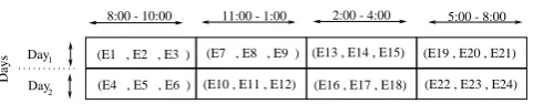
In our example, the 24 exams are scheduled in 2 examination days over 4 examination periods each day. This is depicted in Fig. 2.
Day Day
Days
Periods
1
2
8:00 - 10:00 11:00 - 1:00 2:00 - 4:00 5:00 - 8:00
(E1 , E2 , E3 )
(E4 , E5 , E6 ) (E22 , E23 , E24)
(E19 , E20 , E21)
(E16 , E17 , E18) (E13 , E14 , E15) (E7 , E8 , E9 )
[image:9.595.172.413.282.329.2](E10 , E11 , E12)
Figure 2. Example Schedule with 24 exams
The exams are denoted by the LetterE concatenated to the course code. For example if we have a course code
CS111 then exam code for this course will beECS111. ExamE9 in the picture above is scheduled from 11:00 am to 1:00 pm of Day1. As stated before, in each day we have 3 exams at each period, this is because we have 3
examination rooms available and we wish to maximize their utilization by always allocating non-scheduled exams to the empty rooms.
Depending on the number of exams to be scheduled, a case frequently appears where we sometimes end up by having rooms which are not allocated to any exam at the final examination day. This is logical since the number of exams might not be a multiple of the size of the matrixSched[i,j]. We accommodate for this by adding virtual exams in the remaining empty cells while building our initial solution. These exams have no conflicts whatsoever with any of the other exams. This is done to allow for the algorithm to run onMatlabsince it is necessary to fill-in all matrix cells.
In some other cases, the examination rooms are vast halls, and might hold more thanoneexam atoneperiod. To account for this change, we consider the hall to be multiple examination rooms (the exact multiple depends on the number of seats in the Hall).1
We have provided a function ReturnConflicts(Exam1, Exam2) that takes 2 exams as parameter and returns an integer equal to the number of students taking these exams in common. Using the notation of Subsection 2.1 the function is be described as follows:
Function 1 ReturnConflicts(ea, eb)
set counter = 0
forallsj ∈Sdo
if seja = 1&&sejb = 1then
counter = counter + 1
end if end for
returncounter
We start by inserting the exams to be scheduled into the matrixSched[i,j] randomly and we calculate the cost of this random solution.
The cost of an examination schedule is the sum of:
• the cost of its hard constraints returned by checking for any students having exam clashing (more than one
exam in the same time-slot), and
1Allocation of exams to rooms is done by assigning the next largest (seating) room to the exam having the highest number of
• a fraction of the cost of its soft constraints. This is done by multiplying the cost of these soft constraints by a decimal ε∈]0,1[
This is illustrated below:
T otal Cost=cost of hard constraints+ε·cost of sof t constraints (11)
Still remains to explain how to calculate the cost of the hard and soft constraints of the examination schedule. The cost of the hard constraints is the sum of the values returned after running the function ReturnConflicts() for all pairs of exams occurring in the same time-slot of the same day in the examination schedule. As for the soft constraints, we need to make sure that we space the exams fairly and evenly across the whole group of students thus, we need to check if a student has more than one exam in two consecutive time-slots of the same day. The cost of the soft constraints is the sum of the values returned after running the function ReturnConflicts() for all pairs of exams occurring in theconsecutive time-slots of the same day.
To control the relative importance of the hard constraints over the soft constraints, we multiplied the cost of the soft constraints by a decimalε∈]0,1[.
Once we have defined how to calculate the cost of the solution in hand, we can now use the SA algorithm to iterate over neighbor solutions in the aim of reaching better cost solutions. This is describe in the following subsections.
5.1.1 Choosing a starting temperature
We used the Tuning for initial temperature method as described in [41], whereby we start at a very high temperature and then cool it rapidly until about 60% of worst solutions are being accepted. we then use this temperature as T0.
5.1.2 Temperature Decrement
We used a method which was first suggested by Lundy[42] in1986 to decrement the temperature. The method consists of doing only one iteration at each temperature, but to decrease the temperature very slowly. The formula that illustrates this method is the following:
Ti+1=
Ti 1 +β·Ti
(12) where β is a suitably small value and Ti is the temperature at iterationi.
In our test case we will takeβ to be equal to 0.001. Another possible solution to the temperature decrement is to dynamically change the number of iterations as the algorithm progresses[16].
5.1.3 Final Temperature
As a final temperature Tf, we chose a suitably low temperature where the system gets frozen at. We used similar results as those found in [12] where many experiments using SA were run to solve the university timetabling problem. In [12] each experiment was done using different final temperatures, namely [0.5, 0.05, 0.005, 0.0005, 0.00005] and a fixed value ofTf = 0.005 was chosen since this temperature returned the best solution cost. In our solution, we used the sameTf even though any temperature T∈[0.005,. . . ,1] would have given very close results. But our stopping criterion did not only depend onTf. A check was also made on consecutive solutions where no moves appeared to be improving the cost afterwards and, whenever we received the same cost over more than (T0/4) number of iterations we stopped since we probably have reached a best-case solution. Of course we would
also stop whenever we reach a schedule with cost equalzerosince that would be an optimal solution.
5.1.4 Neighborhood structure
6
ACO Applied To The Scheduling Problem
6.1
Our Approach Using ACOIn this approach we use the same definition of the scheduling problem as the one described in Section 1 and 2. Furthermore, we consider the same example problem as in Subsection 5.1 whereby Sched[i,j] denotes the examination schedule we are building, and ReturnConflicts(Exam1, Exam2) is the function returning an integer equal to the number of students takingExam1, Exam2 in common. We also recap that we are trying to schedule 24 exams in a period of 2 examination days.
To be able to use theACO algorithm on this problem, we create a 24×24 matrix to hold the pheromone values between the exams and call itPhMatrix.
The pheromone values in thetimetablingproblem will be used differently than what has been done in theTSP
example described before since the relative position of an exam does not only depend on its direct predecessor or its direct successor in the schedule, but also on all the exams that are to be scheduled within the same time-slot of the same day (that is in the same set Sij) and therefore the costs are calculated differently in thesetwo problems. The differences are highlighted in the example below:
To calculate the cost of going from a cityi to another cityj in aTSP, at each step we only need to check for the cost related to the distance between these two cities without considering the cost of moving between these cities and the other cities we have previously visited. On the other hand, to calculate the cost of scheduling exams in the same set Sij we must check for all the conflicts between all the exam in this set, at each step when adding an exam to the set.
In the context of the scheduling problem, the ants will therefore decide which exams are feasible to be placed in the same set Sij of the schedule. We know that we can have as many exams in each Sij as there are available rooms.
PhMatrix is first initialized so that the valuesτij :i, j∈ {1, . . . , n} are all equal to 1. The attractivenessηij is defined as follows:
ηij=
1
ReturnConf licts(Ei, Ej)
(13)
whereEi, Ej refer to exams i andj respectively.
At each iteration the ants will start from a new source (exam) and build their solution (schedule). The ants choose an exam as a source; they move to the next exam which has a highest probability according to (8). It is clear that during the first iteration the ants will choose the next exam having the minimum number of conflicts (highestηij) with the previous one, since the pheromone values are all equal.
Once the next exam is chosen by antk, the previous one in the schedule is put in thetabu list of antk, that is a list containing all moves which are infeasible for antk. This is done to ensure that the same exam is not scheduled twice in the timetable. Antk continues its colony, and chooses the next exam in the same way.
Choosing the next exam having the minimum number of conflicts (highest ηij) with the previous one might work for adjacent exams in the schedule, but might also lead to conflicts with other exams scheduled in the same time-slot. So even whenηijis optimal between two consecutive exams, it leads in some cases to high costs returned from conflicts with other exams scheduled within the same Sij. It is possible to account for this problem by elevating the defined parameterαin (8), but this is does not solve the problem completely.
Therefore, a global pheromone evaluation rule is proposed where an antk at examithat has to decide about the next examj of the permutation, makes the selection probability:
• Considering every examj not in the tabu list ofk
• Depending on the sum of all pheromone values between, the exams already scheduled in the same set as i
(denoted byl) and the candidate examj, which is: ∑il=1τlj. So we end up by the following equation:
pij =
(∑il=1τlj)α·η β ij
∑
z∈S(
∑i
l=1τlz)α·η
β iz
∀j ∈S (14)
This makes sure that, starting from past scheduled exam, we have calculated the probabilities and costs of moving to the next exam, between all the exams already scheduled in the same time-slot of the current day and the candidate exam to be added to the schedule, before choosing it.
6.2
Pheromone UpdateAfter scheduling a set of exams (one cell) in the timetableSched[i,j] , we do alocal pheromone update whereby we update the pheromone values between all pairs of scheduled exams according to (10).
On the other hand, to avoid unfeasible distributions (with conflicting exams that lead to dead-end configuration) from being placed in the same set Sij, we have decided to induce negative pheromone values between the exams leading to such distributions in such a way that, if exam i and j lead to future conflicting configurations in the timetable, they will be assigned a negative pheromone valueτij even ifi andj have no conflicts with each other.
The negative pheromone update equation is the inverse of (10) where the addition is replaced by a substraction. The equation is the following:
τij = (1−φ)·τij−φ·τold (15) where φ ∈ (0, 1] is the pheromone decay coefficient, and τold is the old value of the pheromone. This negative pheromone update can be induced directly after the pheromone initialization between the exams resulting in conflicting configurations, therefore before the ants start building their solution. This will ensure that for ant k
the probability of choosing these exams in the same set is very low.
Using the above results of our new approach, the extended form of algorithm 3 would look like the following:
Algorithm 4ACO using our new approach
1.Initialization - Initialize Pheromone and Attractiveness values between exams
∀(ei,ej)∈E,τeiej = 1 andηeiej = 1/ReturnConflicts(ei, ej) Create a random timetable
ford = 1;++;number of days
forj = 1;++;number of periods per day
Sched[d,j]←(e#,e#,e#) where e#is any non-assigned exam
end for end for
Initialize number of ants
K=k1,. . . ,kn and|K|= 50
2.Construct timetable
Foreach ant k∈Kdo
repeat
choose source exam ei from E not in tabuk
choose the next exam ei+1 to move to by means of (14)
append the chosen move to the kthant’s set tabuk until k has scheduled all exams
3. Trail update
∀ (ei,ej) ∈E, update τeiej according to a- Eq. (10) if ReturnConflicts(ei, ej)<1 b- Eq. (15) otherwise
end for
4.Terminating condition
Repeat until we reach a feasible timetable or go back to step 2
7
Empirical Results
We have run the SA algorithm on the exam scheduling problem using the variables and values defined in the preceding sections, and plotted the results in Matlab. A plot showing the variation in the cost values of the examination schedule with respect to a temperature decrement going down from 100 to 0 is shown in Fig. 3. This plot corresponds to an example of running the SA algorithm on an exam schedule without black-listing neighbor schedule configurations that might return high and impractical costs.
Figure 3. Variation in cost values with respect to temperature decrement
[image:13.595.194.392.235.343.2]Another plot is shown in Fig. 4, where the SA algorithm is started from the same initial configuration and run within the same range of temperatures, but now using the improved version that consists of constraining unfeasible neighbor configurations that might return high and impractical costs.
Figure 4. Variation in cost values with respect to temperature decrement after constraining unfeasible neighbor configurations
We can see that the differences between the costs in adjacent temperatures is narrower than those in Fig. 3. Even though the final cost has almost the same value in both examples, but the cost function drops more strictly with respect to temperature when using the improved version. This resulted from the fact that many non-useful iterations were avoided due to the restricting unfeasible configurations.
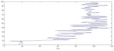
On the other hand, the results of running the ACO algorithm on the example described previously were also plotted on Matlab. Fig. 5 below shows the variation in the cost of the schedule at several iterations. At each iteration we start from a different nest (source) and build a complete solution. Note that in this example the schedule instance chosen contains a huge number of conflicts between students’ exams.
Figure 5. ACO - Cost values at subsequent iterations (High conflict schedule)
We can see that the cost drops significantly from a value around 120 to almost 5 after 100 iterations. We have also run the ACO algorithm on a different instance having a lower number (still a considerable number) of conflicts between exams and the results are plotted in Fig. 6. The initial solution has a cost equal to 20 and it drops to
zeroafter only 45 iterations, therefore an optimal solution was reached.
8
Performance Analysis: ACO vs. SA
Each of theSimulated AnnealingandAnt Colony Optimization algorithms was tested by performing 15 trials in the aim of building complete examination schedules, starting from different initial configurations and using different numbers of exams. The first 5 trials consisted of generating schedules for 24 exams (timetable size = 24) in the minimum possible timescale. In the next 5 trials, we generated timetables of size equal to 32, while in the last 5 trials we generated timetables of size equal to 38.
[image:13.595.194.392.491.580.2]0 5 10 15 20 25 30 35 40 45
50 55 60 65 70 75 80 85 90 95 100
[image:14.595.211.405.61.171.2]Cost
Figure 6. ACO - Cost values at subsequent iterations (Low conflict schedule)
The results with the lowest cost were recorded at each trial, together with their corresponding CPU running time. The standard deviation (σ) of every group of 5 trials was also calculated. All the trials were run on a Core2-DuoPC with 2.0GHzCPU and 2.0GBofRAM. The results are shown in Table 1 below.
Table 1. Performance ofACO andSAalgorithms: Empirical Results.
SA- Running Time(sec) Cost ACO- Running Time(sec) Cost
Trial#1 1.5444 3.55 - 0.2028 0.0100
Trial#2 1.5000 6.80 - 0.2184 1.0500
Trial#3 1.2948 3.70 - 0.1716 10.900
Trial#4 1.5132 3.80 - 0.2184 2.9500
Trial#5 1.5288 3.85 - 0.0936 5.9500
- - σ= 1.37 - - σ= 4.38
SA- Running Time(sec) Cost ACO- Running Time(sec) Cost
Trial#6 2.1300 3.97 - 0.3400 11.8000
Trial#7 1.9909 5.81 - 0.9909 4.3500
Trial#8 1.9001 7.20 - 0.4411 7.5000
Trial#9 2.0152 3.10 - 0.2214 1.3300
Trial#10 2.1001 4.20 - 0.1999 3.4999
- - σ= 1.63 - - σ= 4.06
SA- Running Time(sec) Cost ACO- Running Time(sec) Cost
Trial#11 2.5120 4.36 - 1.0933 13.950
Trial#12 4.6000 3.37 - 0.9922 4.0011
Trial#13 3.0011 5.11 - 1.0056 2.3500
Trial#14 3.3111 3.91 - 0.8851 5.9500
Trial#15 2.7222 3.56 - 0.9111 2.7600
- - σ= 0.69 - - σ= 4.76
We have made the following observations:
1. The running times of ACO are better than those of SA in all 15 trials. SA annealing takes more time to discover and evaluate the neighbor solutions at each iteration (temperature). ACO uses information from prior iterations to guide subsequent colonies to new states (neighbors) which reduces the processing time needed to calculate the cost of such moves.
2. ACO found the least cost solution in all three timetable sizes, even though it sometimes lead to high cost solutions compared to those found in SA. The standard deviations of the timetables’ costs produced using SA are lower than those found in the case of ACO which means that SA provided tight results where the cost values of the solutions are close to each other, while ACO gives broad results where the difference between the cost values might be high.
[image:14.595.119.492.306.582.2]4. When the number ofconflicting exams chosen is too high in such a way that more than 70% of the exams have conflicts with each other (not shown in table 1), the ACO algorithm outperforms the SA algorithm. We had to highly increase the number of iterations done at each temperature (using the static strategy of temperature decrement) to allow for the SA algorithm to explore enough neighbors so that it is able to find a better move (neighbor).
5. When the number ofconflicting exams chosen is very loose in such a way that less than 20% of the exams have conflicts with each other (not shown in table 1), both approaches lead to near-optimal solutions. Although ACO converged to a near-optimal solution using 50 ants, its running time was higher than that of SA, since SA reached the stopping criteria in only very few iterations.
9
Conclusion and Future Work
We have used two algorithms namely SA (simulated annealing) and ACO (ant-colony algorithm) to solve the
Scheduling problem. We first introduced the problem and provided its mathematical formulation in Section 2 and then we described the SA and ACO algorithms and illustrated the way they are used to solve combinatorial optimization problems. We presented our approach to solving the scheduling problem using these algorithms in Section 5 and 6. All the results were implemented usingMatlab, and a comparison between the performance and running times of SA and ACO in producing different examination schedules over several trials was depicted in Table 1. The solution we provided was based on an exam scheduling problem model that could be implemented in different academic institutions. It is not difficult to generalize our solution to solve different scheduling problems by performing some minor modifications regarding the variables related the the problem in hand and the resources available. Our future work consists of parallelizing these algorithms in order to improve their running times and also on using a hybridAnt Colony - Simulated Annealingapproach to improve the cost of our solution. We intend to parallelize the two algorithms at the level of data whereby we work on solving sub-problems and then combine them into a bigger low cost problem. We also intend to achieve parallelism at the level of ants when using the ACO algorithm in such a way that ants can work in parallel to find their solution.
REFERENCES
[1] Edmund Burke, Kirk Jackson, Jeff Kingston, and Rupert Weare. Automated university timetabling: the state of the art.The Computer Journal, 40:565–571, 1997.
[2] Carter M.W., Laporte G., Chinneck J.W., and GERAD. A general examination scheduling system. Les Cahiers du
GERAD. 1992.
[3] Ketan Kotecha, Gopi Sanghani, and Nilesh Gambhava. Genetic Algorithm for Airline Crew Scheduling Problem Using Cost-Based Uniform Crossover. pages 84–91. 2004.
[4] P. Surekha, P.R.A. Mohanaraajan, and S. Sumathi. Ant colony optimization for solving combinatorial fuzzy job shop
scheduling problems. InCommunication and Computational Intelligence (INCOCCI), pages 295 –300, dec. 2010.
[5] Jen Huang. Using ant colony optimization to solve train timetabling problem of mass rapid transit. In Journal of
Computer Information Systems, 2006.
[6] Anthony Wren. Scheduling, timetabling and rostering - a special relationship? In Selected papers from the First
International Conference on Practice and Theory of Automated Timetabling, pages 46–75, London, UK, 1996. Springer-Verlag.
[7] Stephen A. Cook. The complexity of theorem-proving procedures. InProceedings of the third annual ACM symposium
on Theory of computing, STOC ’71, pages 151–158, New York, NY, USA, 1971. ACM.
[8] Richard M. Karp. Reducibility among combinatorial problems. In Michael Jnger, Thomas M. Liebling, Denis Naddef, George L. Nemhauser, William R. Pulleyblank, Gerhard Reinelt, Giovanni Rinaldi, and Laurence A. Wolsey, editors,
50 Years of Integer Programming 1958-2008, pages 219–241. Springer Berlin Heidelberg, 2010.
[9] S. Even, A. Itai, and A. Shamir. On the complexity of timetable and multicommodity flow problems. SIAM Journal
on Computing, 5(4):691–703, 1976.
[10] P Brucker and S Knust. In complexity results for scheduling problems. InRobust and Online Large-Scale Optimization,
volume 5868 of Lecture, Last update: 29.06.2009.
[11] Edmund K. Burke, Dave Elliman, Peter H. Ford, and Rupert F. Weare. Examination timetabling in british universities:
a survey. InSelected papers from the First International Conference on Practice and Theory of Automated Timetabling,
pages 76–90, London, UK, UK, 1996. Springer-Verlag.
[13] C. Y. Cheong, K. C. Tan, and B. Veeravalli. A multi-objective evolutionary algorithm for examination timetabling. J. of Scheduling, 12(2):121–146, April 2009.
[14] D. de Werra. An introduction to timetabling. European Journal of Operational research, (19), 1985.
[15] N Metropolis, A Rosenbluth, M Rosenbluth, A Teller, and E Teller. Equations of state calculations by fast computing
machines. The Journal of Chemical Physics, (21):1087–1091, 1953.
[16] Graham Kendall. Artificial intelligence methods: Simulated annealing - introduction, 2002. course run at the The University of Nottingham within the School of Computer Science and IT.
[17] R. W. Eglese. Simulated annealing: a tool for operational research. European Journal of Operational Research, (46),
1990.
[18] Jimmy Lam and Jean marc Delosme. An efficient simulated annealing schedule: implementation and evaluation.
Technical report, 1988.
[19] M. Dorigo. Optimization, learning and natural algorithms. PhD thesis, Politecnico di Milano, Italy, 1992.
[20] Masri Binti Ayob and Ghaith Jaradat. Hybrid ant colony systems for course timetabling problems. InProceedings of
the 2nd conference on data mining and optimization, Universiti Kebangsaan Malaysia, pages 120–126. IEEE, 2009.
[21] Peter Merz and Bernd Freisleben. A comparison of memetic algorithms, tabu search, and ant colonies for the quadratic
assignment problem. InProc. Congress on Evolutionary Computation, IEEE, pages 2063–2070. Press, 1999.
[22] Marco Dorigo and Christian Blum. Ant colony optimization theory: a survey.Theor. Comput. Sci., 344(2-3):243–278,
November 2005.
[23] Karen I. Aardal, Stan P. M. Van Hoesel, Arie M. C. A. Koster, Carlo Mannino, and Antonio Sassano. Models and solution techniques for frequency assignment problems. pages 261–317, 2001.
[24] Marco Dorigo and Thomas Sttzle. The ant colony optimization metaheuristic: algorithms, applications, and advances. InHandbook of Metaheuristics, pages 251–285. Kluwer Academic Publishers, 2002.
[25] Vittorio Maniezzo, Luca Maria Gambardella, and Fabio De Luigi. Ant colony optimization, April 09 2004.
[26] Oscar Castillo, Patricia Melin, Janusz Kacprzyk, and Witold Pedrycz, editors. Soft computing for Hybrid Intelligent
Systems, volume 154 ofStudies in Computational Intelligence. Springer, 2008.
[27] Marc Dorigo and Socha Krzysztof. An introduction to ant colony optimization.IRIDIA Technical Report Series, 2006.
[28] Marco Dorigo, Mauro Birattari, and Thomas Sttzle. Ant colony optimization - artificial ants as a computational
intelligence technique. IEEE COMPUT. INTELL. MAG, 1:28–39, 2006.
[29] Walter J. Gutjahr. First steps to the runtime complexity analysis of ant colony optimization. Comput. Oper. Res.,
35(9):2711–2727, September 2008.
[30] Juan Frausto-Sol´ıs, Federico Alonso-Pecina, and Jaime Mora-Vargas. An efficient simulated annealing algorithm for
feasible solutions of course timetabling. In Proceedings of the 7th Mexican International Conference on Artificial
Intelligence: Advances in Artificial Intelligence, MICAI ’08, pages 675–685, Berlin, Heidelberg, 2008. Springer-Verlag.
[31] Krzysztof Socha, Michael Sampels, and Max Manfrin. Ant algorithms for the university course timetabling problem with
regard to the state-of-the-art. InIn Proc. Third European Workshop on Evolutionary Computation in Combinatorial
Optimization (EvoCOP 2003, pages 334–345. Springer Verlag, 2003.
[32] M. Chiarandini, M. Birattari, K. Socha, and O. Rossi-Doria. An effective hybrid algorithm for university course
timetabling. Journal of Scheduling, 9(5):403–432, October 2006.
[33] Sara Miner, Saleh Elmohamed, and Hon W. Yau. Optimizing timetabling solutions using graph coloring. InNPAC
REU program, 1995.
[34] Philipp Kostuch. The university course timetabling problem with a three-phase approach. In Proceedings of the
5th international conference on Practice and Theory of Automated Timetabling, PATAT’04, pages 109–125, Berlin, Heidelberg, 2005. Springer-Verlag.
[35] M. Gendreau. An Introduction to Tabu Search. In F. Glover and G. Kochenberger, editors,Handbook of Metaheuristics,
chapter 2, pages 37–54. Kluwer Academic Publishers, 2003.
[36] Krzysztof Socha, Joshua Knowles, and Michael Sampels. A max-min ant system for the university course timetabling
problem. InProceedings of the Third International Workshop on Ant Algorithms, ANTS ’02, pages 1–13, London, UK,
UK, 2002. Springer-Verlag.
[37] Olivia Rossi-doria, Michael Sampels, Mauro Birattari, Marco Chiar, Marco Dorigo, Luca M. Gambardella, Joshua Knowles, Max Manfrin, Monaldo Mastrolilli, Ben Paechter, Luis Paquete, and Thomas Stutzle. A comparison of
the performance of different metaheuristics on the timetabling problem. InIn: Proceedings of the 4th International
[38] Salwani Abdullah, Edmund K. Burke, and Barry Mccollum. An investigation of variable neighbourhood search for
university course timetabling. In The 2nd Multidisciplinary International Conference on Scheduling: Theory and
Applications (MISTA), pages 413–427, 2005.
[39] Edmund K Burke, Barry Mccollum, Amnon Meisels, Sanja Petrovic, and Rong Qu. A graph-based hyper-heuristic for
educational timetabling problems. European Journal of Operational Research, 176:177–192, 2007.
[40] Thomas H. Cormen, Charles E. Leiserson, Ronald L. Rivest, and Clifford Stein. Introduction to Algorithms (3. ed.).
MIT Press, 2009.
[41] Eric Poupaert and Yves Deville. Simulated annealing with estimated temperature.AI Commun., 13(1):19–26, October
2000.