Unification of the complex Langevin method and the
Lefschetz-thimble method
Jun Nishimura1,2,⋆and Shinji Shimasaki1,3
1KEK Theory Center, High Energy Accelerator Research Organization, 1-1 Oho, Tsukuba, Ibaraki 305-0801, Japan
2Graduate University for Advanced Studies (SOKENDAI), 1-1 Oho, Tsukuba, Ibaraki 305-0801, Japan
3Research and Education Center for Natural Sciences, Keio University, Hiyoshi 4-1-1, Yokohama, Kanagawa 223-8521, Japan
Abstract. Recently there has been remarkable progress in solving the sign problem, which occurs in investigating statistical systems with a complex weight. The two promis-ing methods, the complex Langevin method and the Lefschetz thimble method, share the idea of complexifying the dynamical variables, but their relationship has not been clear. Here we propose a unified formulation, in which the sign problem is taken care of by both the Langevin dynamics and the holomorphic gradient flow. We apply our formulation to a simple model in three different ways and show that one of them interpolates the two methods by changing the flow time.
1 Introduction
Recently there has been remarkable development in solving the sign problem. Suppose we consider a path integral
Z=
dxw(x), (1)
in which the integration contour is taken to be the real axis and the integrandw(x) is a complex number. When the phase ofw(x) oscillates violently, it is extremely hard to evaluate the integral by Monte Carlo methods using the reweighting formula due to huge cancellations between configurations sampled with the Boltzmann weight|w(x)|. This is the sign problem. The key idea in recent development is to
complexify the dynamical variables.
In the generalized Lefschetz-thimble method (GLTM) [1,2], the sign problem is minimized by deforming the integration contour. Namely, the integration contour is determined by solving the holomorphic gradient flow, which makes the phase oscillation of the integrand much milder. The remaining phase oscillation can be dealt with by the standard reweighting method. In the complex Langevin method (CLM) [3,4], on the other hand, one defines a stochastic process in the complex plane in such a way that the ensemble average using configurations after thermalization gives the expectation value with respect to the original path integral. Unlike the GLTM, there is no remaining
phase to take care of. However, the equivalence to the original path integral requires certain conditions [5,6,7], which limit the applicability of the method. Here we propose a unified formulation [8], which clarifies the relationship between the two methods.
The rest of this article is organized as follows. In section2we briefly review the CLM and the GLTM. In section3 we present our formulation, which unifies the two methods. In section4 we apply our formulation to a single-variable case and clarify the relationship between the two methods. Section5is devoted to a summary and discussions.
2 Brief review of the CLM and the GLTM
In this section, we briefly review the CLM and the GLTM. Here we consider a general model given by a multi-variable integral
Z=
Rn
dx e−S(x)
, (2)
where the actionS(x) is a complex function ofx =(x1,· · · ,xn) ∈ Rn. The expectation value of an observableO(x) is defined by
�O(x)�= 1 Z
Rn
dxO(x)e−S(x). (3)
2.1 Complex Langevin Method (CLM)
In the CLM [3,4], we complexify the dynamical variablesx∈Rnasx→z=x+iy∈Cnand extend the action and the observable to holomorphic functions ofz. Then we consider the complex Langevin equation
∂
∂tzk(t)=− ∂S(z)
∂zk +ηk(t), (4)
wheretis a fictitious time andηk(t) is a real Gaussian noise normalized as�ηk(t)ηl(t′)�η=2δklδ(t−t′).
This equation (4) defines a probability distribution ofzat each timet. It is shown [5,6] that under certain conditions, the expectation value�O(x)�in the original integral (3) can be obtained as
�O(x)�=�O(z)�CLM, (5)
where the right-hand side denotes the expectation value ofO(z) with respect to the limiting distribution
ofzatt→ ∞. As in the case of Monte Carlo methods,�O(z)�CLMcan be replaced with a long-time
average of the observable calculated for the generated configurationsz(t) if ergodicity holds for the Langevin time-evolution. When the actionS(x) is real, this method reduces to the (real) Langevin method, which is a standard Monte Carlo algorithm.
phase to take care of. However, the equivalence to the original path integral requires certain conditions [5,6,7], which limit the applicability of the method. Here we propose a unified formulation [8], which clarifies the relationship between the two methods.
The rest of this article is organized as follows. In section2 we briefly review the CLM and the GLTM. In section3 we present our formulation, which unifies the two methods. In section4 we apply our formulation to a single-variable case and clarify the relationship between the two methods. Section5is devoted to a summary and discussions.
2 Brief review of the CLM and the GLTM
In this section, we briefly review the CLM and the GLTM. Here we consider a general model given by a multi-variable integral
Z=
Rn
dx e−S(x)
, (2)
where the actionS(x) is a complex function ofx =(x1,· · ·,xn) ∈ Rn. The expectation value of an observableO(x) is defined by
�O(x)�= 1 Z
Rn
dxO(x)e−S(x). (3)
2.1 Complex Langevin Method (CLM)
In the CLM [3,4], we complexify the dynamical variablesx∈Rnas x→z=x+iy∈Cnand extend the action and the observable to holomorphic functions ofz. Then we consider the complex Langevin equation
∂
∂tzk(t)=− ∂S(z)
∂zk +ηk(t), (4)
wheretis a fictitious time andηk(t) is a real Gaussian noise normalized as�ηk(t)ηl(t′)�η=2δklδ(t−t′).
This equation (4) defines a probability distribution ofzat each timet. It is shown [5,6] that under certain conditions, the expectation value�O(x)�in the original integral (3) can be obtained as
�O(x)�=�O(z)�CLM, (5)
where the right-hand side denotes the expectation value ofO(z) with respect to the limiting distribution
ofzatt→ ∞. As in the case of Monte Carlo methods,�O(z)�CLMcan be replaced with a long-time
average of the observable calculated for the generated configurationsz(t) if ergodicity holds for the Langevin time-evolution. When the actionS(x) is real, this method reduces to the (real) Langevin method, which is a standard Monte Carlo algorithm.
The derivation of the equality (5) uses integration by parts, which can be justified if the distribution ofzfalls offfast enough in the imaginary directions [5,6] as well as near the singularities of the drift term if they exist [9,10]. Recently [7], a subtlety in the use of time-evolved observables in the original argument [5,6] was pointed out, and the derivation of the equality (5) has been refined taking account of this subtlety. This also led to the proposal of a useful criterion for justification, which states that the distribution of the drift term should be suppressed exponentially or faster at large magnitude [7].
2.2 Generalized Lefschetz-Thimble Method (GLTM)
In the GLTM [2], we deform the integration contour fromRnto ann-dimensional real manifold inCn by using the so-called holomorphic gradient flow, which makes the sign problem milder.
The holomorphic gradient flow is defined by the differential equation
∂
∂σφk(x;σ)=
∂S(φ(x;σ)) ∂φk
, (6)
which is solved from σ = 0 to σ = τ with the initial condition φ(x; 0) = x ∈ Rn. The flowed configurations define an-dimensional real manifold inCn, which we denote asMτ={φ(x;τ)|x∈Rn}.
One can actually argue that the integration contour can be deformed continuously fromRntoMτ⊂Cn without changing the partition function. Then, by noting thatφ(x)≡φ(x;τ) defines a one-to-one map fromx∈Rntoφ∈Mτ, one can rewrite the partition function as
Z=
Mτdφe
−S(φ)
=
Rn
dxdetJ(x)e−S(φ(x)), (7)
whereJkl(x) is the Jacobian corresponding to the mapφ(x). Thus, the deformation of the integration contour simply amounts to changing the action fromS(x) to the “effective action”
Seff(x)=S(φ(x))−log detJ(x). (8) The virtue of using the holomorphic gradient flow (6) in deforming the integration contour lies in the fact that the real part of the actionS grows monotonically along the flow keeping the imaginary part constant. Thus, for a sufficiently large flow timeτ, the partition function (7) is dominated by a small region ofx, and the sign problem becomes much milder. One can therefore apply a standard Monte Carlo method using only the real part of the effective action (8), dealing with the imaginary part by reweighting. Thus, the expectation value ofO(x) can be calculated as
�O(x)�= �e
−iImSeff(x)O(φ(x;τ))�MC
�e−iImSeff(x)�
MC , (9)
where�· · · �MC represents the expectation value obtained by a Monte Carlo method with the weight
exp(−ReSeff(x)).
When the flow timeτbecomes infinitely large, Mτcontracts to a set of Lefschetz thimbles, and
the GLTM reduces to the so-called Lefschetz-thimble method [1]. Since ImS(φ(x)) is constant on each thimble, the sign problem is maximally reduced in some sense. However, when there are more than one thimbles, the transition between thimbles does not occur during the Monte Carlo simulation, which leads to the violation of ergodicity. The GLTM [2] avoids this problem of the original method by choosing a large but finite flow time. Recently, it has been pointed out [11,12] that the flow time can be made as large as one wishes without the ergodicity problem if one uses the parallel tempering algorithm.
Let us here compare the two methods. From the viewpoint of solving the sign problem, the CLM is more powerful since it solves it completely as far as it works, whereas the GLTM has a residual sign problem, which may be problematic when the system size becomes large. From the viewpoint of numerical cost, the GLTM is more demanding since one has to calculate the Jacobian arising from deforming the integration contour. It should also be noted that one can include fermions in the CLM with the cost of O(V) for the system sizeV, whereas in the GLTM, it requires O(V3). The disadvantage
In this situation, it is useful to clarify the relationship between the two methods. Note here that despite the resemblance of the two methods in that they both use complexified variables, the connec-tion between them is far from obvious. In particular, the CLM samples configuraconnec-tions in the complex plane based on the Langevin process, whereas the GLTM samples configurations on a particular con-tour in the complex plane obtained by deforming the original concon-tour along the real axis. Therefore the dimension of the configuration space in the CLM is twice as large as that of the GLTM.
3 Unifying the CLM and the GLTM
In this section, we present our formulation, which unifies the CLM and the GLTM. The basic idea is to apply the CLM to the partition function (7) that appears in the GLTM. The real variablesx∈Rn parametrizing then-dimensional real manifold in Cn have to be complexified, and they evolve in time following the complex Langevin equation obtained from the effective action (8). The observable should be evaluated with the flowed configurationφ(z), which is defined as holomorphic extension of φ(x). Therefore, it is important to see how the distribution of flowed configurations changes as the flow time increases.
We apply the CLM to the partition function (7) by considering the drift term
∂Seff(x) ∂xk =
∂S(φ(x))
∂φl Jlk(x)−J
−1
lm(x)Kmlk(x), (10)
where we have definedKmlk(x)≡∂Jml(x;τ)/∂xk. In order to evaluate this function at complex values z, we need to defineφ(z), Jkl(z) and Kmlk(z) as holomorphic extension ofφ(x), Jkl(x) andKmlk(x), respectively.
Let us note here that the flow equation (6) forφ(x) involves complex conjugation on the right-hand side. Therefore, in order to defineφ(z;σ) as holomorphic functions ofz, we have to extend the flow equations as
∂
∂σφk(z;σ)=
∂S(φ(¯z;σ)) ∂φk
, (11)
whereφ(¯z;σ) appears on the right-hand side. This function with ¯zin the argument obeys the flow equation, which can be obtained by replacingzwith ¯zin the above equation. In practice, we solve the two sets of equations simultaneously with the initial conditionsφ(z; 0)=zfor a particular value ofz at each Langevin step. The same trick can be used to obtainJkl(z;σ) andKmlk(z;σ) as well.
Using this formulation, we can calculate the expectation value (3) as
�O(x)�=�O(φ(z;τ))�CLM, (12)
where the flowed configurationφ(z;τ) has to be used in evaluating the observable unlike in the ordi-nary CLM (5). Forτ=0, our formulation reduces to the ordinary CLM sinceφ(z; 0)=z,Jkl(z; 0)=δkl andKklm(z; 0)=0.
4 Results for a single-variable model
In this section, we apply our unified formulation to a single-variable model to clarify the relationship between the CLM and the GLTM. The model is defined by the partition function [7,9,10],
Z=
In this situation, it is useful to clarify the relationship between the two methods. Note here that despite the resemblance of the two methods in that they both use complexified variables, the connec-tion between them is far from obvious. In particular, the CLM samples configuraconnec-tions in the complex plane based on the Langevin process, whereas the GLTM samples configurations on a particular con-tour in the complex plane obtained by deforming the original concon-tour along the real axis. Therefore the dimension of the configuration space in the CLM is twice as large as that of the GLTM.
3 Unifying the CLM and the GLTM
In this section, we present our formulation, which unifies the CLM and the GLTM. The basic idea is to apply the CLM to the partition function (7) that appears in the GLTM. The real variablesx∈Rn parametrizing then-dimensional real manifold in Cn have to be complexified, and they evolve in time following the complex Langevin equation obtained from the effective action (8). The observable should be evaluated with the flowed configurationφ(z), which is defined as holomorphic extension of φ(x). Therefore, it is important to see how the distribution of flowed configurations changes as the flow time increases.
We apply the CLM to the partition function (7) by considering the drift term
∂Seff(x) ∂xk =
∂S(φ(x))
∂φl Jlk(x)−J
−1
lm(x)Kmlk(x), (10)
where we have definedKmlk(x)≡∂Jml(x;τ)/∂xk. In order to evaluate this function at complex values z, we need to defineφ(z), Jkl(z) andKmlk(z) as holomorphic extension ofφ(x), Jkl(x) andKmlk(x), respectively.
Let us note here that the flow equation (6) forφ(x) involves complex conjugation on the right-hand side. Therefore, in order to defineφ(z;σ) as holomorphic functions ofz, we have to extend the flow equations as
∂
∂σφk(z;σ)=
∂S(φ(¯z;σ)) ∂φk
, (11)
whereφ(¯z;σ) appears on the right-hand side. This function with ¯zin the argument obeys the flow equation, which can be obtained by replacingzwith ¯zin the above equation. In practice, we solve the two sets of equations simultaneously with the initial conditionsφ(z; 0)=zfor a particular value ofz at each Langevin step. The same trick can be used to obtainJkl(z;σ) andKmlk(z;σ) as well.
Using this formulation, we can calculate the expectation value (3) as
�O(x)�=�O(φ(z;τ))�CLM, (12)
where the flowed configurationφ(z;τ) has to be used in evaluating the observable unlike in the ordi-nary CLM (5). Forτ=0, our formulation reduces to the ordinary CLM sinceφ(z; 0)=z,Jkl(z; 0)=δkl andKklm(z; 0)=0.
4 Results for a single-variable model
In this section, we apply our unified formulation to a single-variable model to clarify the relationship between the CLM and the GLTM. The model is defined by the partition function [7,9,10],
Z=
dx(x+iα)pe−x2/2, (13)
-1.5 -1 -0.5 0
-4 -3 -2 -1 0 1 2 3 4
τ=0
-1.5 -1 -0.5 0
-4 -3 -2 -1 0 1 2 3 4
τ=3
-1.5 -1 -0.5 0
-4 -3 -2 -1 0 1 2 3 4
τ=6
-1.5 -1 -0.5 0
-4 -3 -2 -1 0 1 2 3 4
τ=9
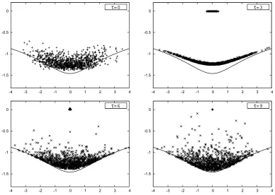
Figure 1.The distribution ofz(represented by “+”) and flowed configurations (represented by “×”) obtained by
applying the CLM to (14) are plotted forτ=0,3,6,9 from Top-Left to Bottom-Right. The solid line represents the Lefschetz thimble. Atτ=0, the distribution ofzand flowed configurations coincides.
wherexis a real variable, whileαand pare real parameters. Whenα 0 and p 0, the weight
becomes complex and the sign problem occurs.
First, using the holomorphic gradient flow for a fixed flow timeτ, we rewrite (13) as
Z=
dx J(x) (φ(x)+iα)pe−φ(x)2/2, (14)
whereφ(x) =φ(x;τ) is obtained by solving (6) forφ(x;σ). Here we consider three versions of our formulation; namely
(i) CLM applied to the model (14).
(ii) CLM applied to the partially phase-quenched model:
ZpPQ=
dx|J(x)|(φ(x)+iα)pe−φ(x)2/2. (15)
(iii) RLM applied to the totally phase-quenched model:
ZPQ=
-1.5 -1 -0.5 0
-4 -3 -2 -1 0 1 2 3 4
τ=0
-1.5 -1 -0.5 0
-4 -3 -2 -1 0 1 2 3 4
τ=3
-1.5 -1 -0.5 0
-4 -3 -2 -1 0 1 2 3 4
τ=6
-1.5 -1 -0.5 0
-4 -3 -2 -1 0 1 2 3 4
τ=9
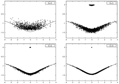
Figure 2. The distribution ofz(represented by “+”) and flowed configurations (represented by “×”) obtained
by applying the CLM to the partially phase quenched model (15) are plotted forτ = 0,3,6,9 from Top-Left to Bottom-Right. The solid line represents the Lefschetz thimble. Atτ =0, the distribution ofzand flowed configurations coincides.
In the cases (ii) and (iii), appropriate reweighting is needed in calculating the expectation value as described in the previous section.
We focus on the choice of parametersp=4 andα=4.2, for which there exists only one Lefschetz thimble and the ordinary CLM is known to be justified [7]. The flow equation (11) and those for Jkl(z;σ) andKmlk(z;σ) are solved forτ=0,3,6,9. For the details of the simulation, see ref. [8]. In figures1,2and3, we show the distribution ofzand flowed configurations obtained in the case (i), (ii) and (iii), respectively.
-1.5 -1 -0.5 0
-4 -3 -2 -1 0 1 2 3 4
τ=0
-1.5 -1 -0.5 0
-4 -3 -2 -1 0 1 2 3 4
τ=3
-1.5 -1 -0.5 0
-4 -3 -2 -1 0 1 2 3 4
τ=6
-1.5 -1 -0.5 0
-4 -3 -2 -1 0 1 2 3 4
τ=9
Figure 2. The distribution ofz(represented by “+”) and flowed configurations (represented by “×”) obtained
by applying the CLM to the partially phase quenched model (15) are plotted forτ = 0,3,6,9 from Top-Left to Bottom-Right. The solid line represents the Lefschetz thimble. Atτ =0, the distribution ofzand flowed configurations coincides.
In the cases (ii) and (iii), appropriate reweighting is needed in calculating the expectation value as described in the previous section.
We focus on the choice of parametersp=4 andα=4.2, for which there exists only one Lefschetz thimble and the ordinary CLM is known to be justified [7]. The flow equation (11) and those for Jkl(z;σ) andKmlk(z;σ) are solved forτ=0,3,6,9. For the details of the simulation, see ref. [8]. In figures1,2and3, we show the distribution ofzand flowed configurations obtained in the case (i), (ii) and (iii), respectively.
Let us first discuss the case (i) shown in figure1. Atτ = 0, the distribution ofφ(z;τ = 0)= z is nothing but that of the ordinary CLM. Atτ=3, the distribution ofzcomes close to the real axis, which occurs because the sign problem is reduced to large extent by the holomorphic gradient flow. As a result of this, the distribution ofφ(z;τ) comes close to a curve, which looks similar to the one obtained in the GLTM for the sameτshown in figure3. At largerτ, however, the distribution of φ(z;τ) spreads out again, and its boundary approaches the Lefschetz thimble. The spreading of the distribution can be understood as the effects of the complex Langevin dynamics, which takes care of the residual sign problem arising from the Jacobian even in the large-τlimit. The distribution of z shrinks towards the origin, but the zoom up shows that it does not contract to a distribution on the real axis [8]. It is interesting that the expectation values evaluated with flowed configurationsφ(z;τ)
-1.5 -1 -0.5 0
-4 -3 -2 -1 0 1 2 3 4
τ=0
-1.5 -1 -0.5 0
-4 -3 -2 -1 0 1 2 3 4
τ=3
-1.5 -1 -0.5 0
-4 -3 -2 -1 0 1 2 3 4
τ=6
-1.5 -1 -0.5 0
-4 -3 -2 -1 0 1 2 3 4
τ=9
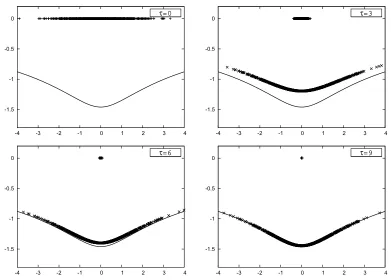
Figure 3. The distribution ofz(represented by “+”) and flowed configurations (represented by “×”) obtained
by applying the RLM to the phase quenched model (16) are plotted forτ=0,3,6,9 from Top-Left to Bottom-Right. The solid line represents the Lefschetz thimble. Atτ=0, the distribution ofzand flowed configurations coincides.
reproduce the exact results for anyτwithout reweighting although the distribution ofφ(z;τ) looks quite different for differentτ.
The case (ii) shown in figure2 is of particular interest. Atτ = 0, the distribution ofφ(z;τ = 0)=zis nothing but that of the ordinary CLM, as in the case (i). Asτincreases, the distribution of φ(z;τ) approaches the Lefschetz thimble, while the distribution ofzapproaches the real axis (See also the Appendix of ref. [8].). This is due to the fact that the sign problem that the complex Langevin dynamics has to take care of vanishes in the largeτlimit since the phase of the Jacobian is taken care of by reweighting and the remaining phase factor is taken care of by the holomorphic gradient flow. Thus, in this case our unified formulation interpolates the CLM and the original Lefschetz-thimble method via the flow time.
In the case (iii) shown in figure3, our formulation reduces to the GLTM [2]. At τ = 0, the calculation simply amounts to applying the reweighting method to the original model (13). Atτ >0, the distribution ofφ(x;τ) is restricted to the deformed integration contourMτ, which approaches the
5 Summary and discussions
We have proposed a formulation which unifies the CLM and the GLTM by applying the CLM to the real variables that parametrize the deformed integration contour in the GLTM. The residual sign problem in the GLTM is treated in three different ways. We have applied the three versions to a single-variable model in the case with a single Lefschetz thimble, and investigated the distribution of flowed configurations, which are used in evaluating the observables. In particular, we have found that the second version interpolates the ordinary CLM and the original Lefschetz-thimble method.
While our formulation is useful in clarifying the relationship between the CLM and the GLTM, it is not of much practical use since the computational cost required in solving the differential equations forφ(z;σ),Jkl(z;σ) andKmlk(z;σ) increases asO(V),O(V3) andO(V5), respectively, with the system sizeV. Note also that the computational cost increases linearly with the flow time. Furthermore, our formulation as it stands does not help in enlarging the range of applicability of the CLM [5,6,7]. The reason for this is that the distribution of flowed configurations is qualitatively not much different from the distribution of configurations obtained in the CLM, which is nothing but the distribution obtained forτ = 0 in the first and second versions of our formulation. For instance, in the model (13) it is known that the CLM gives wrong results forα3.7 withp=4 due to the singular drift problem [7]. This cannot be cured by the first and second versions of our formulation. For largeτ, the situation gets even worse since the flowed configurations tend to come closer to the singularity of the drift term, and the simulation itself becomes unstable. Thus, when the CLM fails, our formulation fails as well, except for the third version, which does not rely on the justification of the CLM.
Nevertheless, we consider that the relationship of the two methods as seen in our unified formula-tion is useful in developing these methods further. In particular, it is possible to generalize the CLM in such a way that the range of applicability is enlarged as we report elsewhere.
References
[1] M. Cristoforetti, F. Di Renzo, L. Scorzato (AuroraScience), Phys. Rev.D86, 074506 (2012), 1205.3996
[2] A. Alexandru, G. Basar, P.F. Bedaque, G.W. Ridgway, N.C. Warrington, JHEP05, 053 (2016), 1512.08764
[3] G. Parisi, Phys. Lett.131B, 393 (1983) [4] J.R. Klauder, Phys. Rev.A29, 2036 (1984)
[5] G. Aarts, E. Seiler, I.O. Stamatescu, Phys. Rev.D81, 054508 (2010),0912.3360
[6] G. Aarts, F.A. James, E. Seiler, I.O. Stamatescu, Eur. Phys. J.C71, 1756 (2011),1101.3270 [7] K. Nagata, J. Nishimura, S. Shimasaki, Phys. Rev.D94, 114515 (2016),1606.07627 [8] J. Nishimura, S. Shimasaki, JHEP06, 023 (2017),1703.09409
[9] J. Nishimura, S. Shimasaki, Phys. Rev.D92, 011501 (2015),1504.08359 [10] G. Aarts, E. Seiler, D. Sexty, I.O. Stamatescu, JHEP05, 044 (2017),1701.02322 [11] M. Fukuma, N. Umeda, PTEP2017, 073B01 (2017),1703.00861