c
Owned by the authors, published by EDP Sciences, 2012
A simple mechanical analysis of the isentropic compression
experiment
F. Montheillet
1and G. Roy
21Ecole Nationale Sup ´erieure des Mines de Saint-Etienne, SMS-EMSE, CNRS UMR 5146, 158 cours Fauriel,´
42023 Saint-Etienne Cedex 2, France
2CEA-Valduc, DRMN, 21120 Is-sur-Tille, France
Abstract. The uniaxial strain compression test, also referred to as isentropic compression experiment, was analyzed using a simple basically analytical model. It accounts for the compression under prescribed loading rate of a single phase elastic, elastic-perfectly plastic, or elastic-viscoplastic material. In each case, stresses, elastic and plastic strain rates, as well as the kinetic, elastic, and plastic powers, were derived and compared.
1 Introduction
The isentropic compression experiment (ICE) has been increasingly used for the investigation of constitutive equa-tions at very large strain rates and under high pressures. To a first approximation, it can be considered as auniaxial strain compression test, where the loading rate can be prescribed for instance by an electromagnetic or laser impulse, or by detonation products stagnation [1, 2]. In such conditions, the deformation of the specimen is both adiabatic (as far as the test duration is sufficiently short) and reversible, by contrast to the classical shock loading experiments. Such conditions are referred to as quasi-isentropic, as plasticity is also likely to occur. A complete thermomechanical analysis of the experiment, including in particular inertia effects and wave propagation, obviously requires numerical computations. Nevertheless, the simple mechanical model proposed below allows to assess the influence of the various loading or material parameters straightforwardly. Purely elastic, elastic-perfectly plastic, and power law viscoplastic single phase materials will be considered.
2 Uniaxial strain compression test
2.1 Geometry and assumptions
Figure 1 shows schematically the uniaxial compression of a cylindrical specimen embedded in a non deformable die. The strains and strain rates can be considered as the sum of two components,viz. an elastic term (Fig. 1b), and a plastic or viscoplastic term (Fig. 1c), which may possibly be zero. The two velocity fields are assumed to be uniform at any time. This precludes wave propagation associated with dynamic loading, but still holds at large strain rates, as far as a material element (elementary representative volume) is considered. Therefore ˙εe
rr =ε˙eθθand ˙ε p rr =ε˙pθθ,
for the elastic and plastic components, respectively, while the non-diagonal components are zero.
2.2 Boundary conditions
They are prescribed in terms of total velocity: ˙ur(R) =
0, where R is the current specimen radius, at any point of the cylindrical boundary, ˙uz(0) = 0 on the lower
horizontal surface of the specimen, and ˙uz(H)=H which˙
is prescribed to the upper surface. More specifically, the following sinusoidal loading kinetics will be applied:
˙ H
H =−ε˙Msin
2π
2tn
(1) where the normalized time tn = t/tM. At final time
tM, the loading rate reaches its maximum value−ε˙M(with
˙
εM > 0). By adding and subtracting the two equations
˙
εrr=ε˙err+ε˙ p
rr=0 and ˙εzz=ε˙ezz+ε˙ p
zz=H/H, and taking˙
into account plastic incompressibility, the two following relations are derived:
2 ˙εerr+ε˙
e
zz=H/H˙ =V/V.˙ (2)
where V denotes the volume of the specimen, and:
˙ εe
rr−ε˙ezz
+
˙ εp
rr−ε˙pzz
=−H/H˙ (3)
Moreover, since ˙εprr=−ε˙err, incompressiblity again implies
˙ εp
zz =2 ˙εerr, which means that the (visco)plastic strain rates
(and strains) can be immediately derived from their elastic counterparts, for any type of inelastic (incompressible) behaviour of the material.
3 Purely elastic behaviour
The material is first assumed isotropic and purely elastic. The Hooke equation:
σ=(κ−2µ/3) tr(εe)δ+2µεe
(4) yields:
σm=2σrr+σzz
3 =κ
2εe rr+εezz
(5) σd=σrr−σzz=2µ
εe rr−εezz
H H
H
(a)
(b)
(c)
e
zz
e
rr
e
rr
e
zz
e
rr
e
rr
∆ε
∆ε
∆ε
p
rr
p
rr
∆ε
p
zz
p
zz
∆ε
p
rr
p
rr
∆ε
Fig. 1.Schematic view of the uniaxial strain (ICE) compression test. (a) Initial state. (b) Elastic strain. (c) Plastic strain.
for the mean and deviatoric stresses, respectively. Assum-ing the elastic moduli κ and µ remain constant during compression, and using Eqs. (2) and (3) after integration with respect to time gives:
σm=κln (H/H0) (7)
and:
σd=−2µln (H/H0) (8)
From the above equations, it is quite easy to derive the stress components σrr andσzz, and the associated strains εe
rrandεezz. In the case of a purely elastic material, closed
form analytical expressions are thus obtained. It will be shown in the next section that it is the same in the case of the elastic-perfectly plastic behaviour.
4 Elastic-perfectly plastic behaviour
The plastic behaviour is assumed to be isotropic, according to the von Mises yield criterion and the associated flow rule. Wheneverσd < σ0, whereσ0 is the von Mises flow
stress, the analysis of 3 still holds. Plastic strain starts when σd=σ0, or, according to Eq. (8):
H H0 =
exp
−σ0
2µ
(9)
In the elastic-plastic range, the mean stress is still given by Eq. (7), whereasσd=σ0remains constant. The stress and
strain components then take the simple form:
σrr=κln
H H0
+ 1 3σ0 σzz=κln
H H0
−2
3σ0
(10)
εe rr=
1 3
lnH H0
+ σ0
2µ
εe zz =
1 3
lnH H0
−σ0
µ
(11)
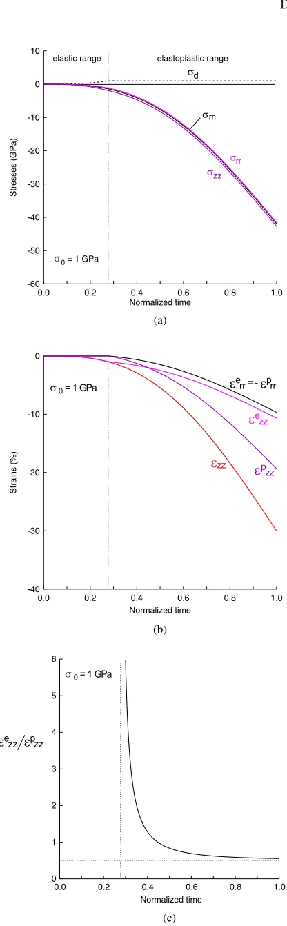
Figure 2a shows the time dependence of the stresses for κ = 140 GPa,µ =50 GPa, andσ0 = 1 GPa. For further
comparisons the loading kinetics was imposed according to (1). It is worth to note, however, that time and strain rate have no influence on the behaviour in the present case. The (positive) deviatoric stress remains much less (σd ≤
1 GPa) than the (negative, i.e. compressive) mean stress amplitude, such that the radial and axial stress components σrrandσzzdo not differ significantly.
Figure 2b shows the associated elastic and plastic strains. In the elastic range,εe
rris zero due to the boundary
conditions. By contrast, in the elastoplastic domain, two radial opposite strains εe
rr < 0 and ε p
rr > 0 contribute to
an overall zero strain, as illustrated in Fig. 1. During the first steps of plastic deformation, the modulus ofεpzzis less
than that ofεe
zz, but the two curves cross at tn ≈0.45 and
the plastic strain axial component becomes increasingly greater than the elastic one. This is also illustrated by Fig. 2c which shows the time dependence of the axial strain ratioRz=εezz/εezzε
p
zz, which is obviously infinite in
the elastic range, then decreases monotonically, and tends to 1/2 at large compression strains.
5 Elastic-viscoplastic material
The more general case of a nonlinearly elastic-viscoplastic material is now considered. Such kind of behaviour is illustrated in Fig. 3, which shows that the overall strain is the sum of an elastic component (spring) and a vis-coplastic component (dashpot). For the sake of simplicity, the threshold σe (yield stress) will be set to zero in the
following, and the viscoplastic behaviour will take the form of a power law:
σ0=kε˙¯m (12)
where ˙¯εis the von Mises equivalent strain rate and m the strain rate sensitivity parameter. When m=0, this model is equivalent to the elastic-perfectly plastic case addressed in section 4. When m = 1, the behaviour is elastic-linearly viscoplastic, which is tantamount forσe = 0, to
the Maxwellviscoelasticmodel.
0.0 0.2 0.4 0.6 0.8 1.0 Normalized time
-60 -50 -40 -30 -20 -10 0 10
Stresses
(G
P
a)
m d
rr
zz
0 = 1 GPa
elastic range elastoplastic range
(a)
0.0 0.2 0.4 0.6 0.8 1.0
Normalized time -40
-30 -20 -10 0
St
rain
s (%
)
(b)
0.0 0.2 0.4 0.6 0.8 1.0
Normalized time 0
1 2 3 4 5 6
(c)
σ
σ
σ
σ
σ
εe rr = - εprr
εezz εpzz
εezz
εpzz εzz
σ0 = 1 GPa
σ0 = 1 GPa
Fig. 2.Time dependence of the stresses (a), the strains (b) and the axial strain ratio (c) for an elastic-perfectly plastic material (see parameters in text).
elastic
ε
nonlinearly viscous
viscoplastic threshold
eσ
pε
σ
elastic
e
viscoplastic threshold
Fig. 3. Schematic representation of the elastic-viscoplastic behaviour.
the second reflects a strain rate sensitivity to the (elastic) volume change. By contrast, in the present model, viscous effects have a purely deviatoric origin.
The deviatoric stresssand plastic strain rate ˙εptensors are related by the flow rule derived from the von Mises yield equation by the normality rule:
s= 2 3
σ0
˙¯ ε ε˙
p
(13) Since the strain rate tensor is diagonal, and taking into account cylindrical symmetry and plastic incompressi-bility, it is easy to show that ˙¯ε=2 ˙εprr=−2 ˙εerr. Taking the inverse of Eq. (13) and using Eqs. (3) and (6) leads to the following differential equation for the unknown function of timeσd:
˙ σd+
3µ k1/m(σd)
1/m=−2µH˙
H (14)
This equation must be solved numerically, except in the linear case m =1. On the other side,σmis still given by
Eq. (7), such that there is no coupling between deviatoric and volumic effects.
Equation (14) was solved for µ = 50 GPa, k = 300 MPa, and various values of m. The loading kinetics was given by Eq. (1), with ˙εM = 103s−1 and tM =
6×10⁻⁴s, leading to a final strainε
M =−0,3. For an initial
thickness H0 =1 mm of the specimen, the final thickness
is HM =0.74 mm.
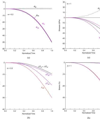
Figures 4a and 5a show the time dependence of the stresses for m = 0.2 and 1, respectively. The deviatoric stress σd, and thus the departure between the radial and
axial stress components, significantly increase with m. It is remarkable that Figs. 4a (m = 0.2) and 2a (elastic-perfectly plastic material) look very similar: this illustrates the continuity of the mechanical behaviour when m de-creases and tends to zero.
The corresponding elastic, plastic, and total strains are depicted in Figs. 4b and 5b. All are negative (compression), to the exception of the radial plastic componentεprrwhich
is not shown in the diagrams. The amplitude of the axial plastic strain εpzz(< 0) is much lower for m = 1 than
0.0 0.2 0.4 0.6 0.8 1.0 Normalized Time
-60 -50 -40 -30 -20 -10 0 10
Stre
sses
(GPa)
m
σ
σ
d
σrr σzz
m = 0.2
(a)
0.0 0.2 0.4 0.6 0.8 1.0
Normalized Time -40
-30 -20 -10 0
St
rain
s
(%
)
εe ε
rr = - prr
εe zz
εp zz
εzz
m = 0.2
(b)
Fig. 4.Time dependence of the stresses (a) and the elastic, plastic, and total strains (b) of a nonlinear (m=0.2) elastic-viscoplastic material.
material) shows the continuity of the material behaviour when m→0.
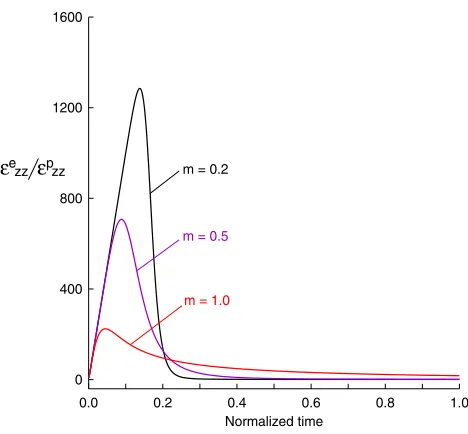
Figure 6 depicts the time evolution of the Rz ratio
for m = 0.2, 0.5, and 1, which confirms the former remarks. Comparison with Fig. 2 shows a mathemat-ical discontinuity of this dependence when m → 0: whenever m is nonzero, the initial value of Rz is zero,
whereas Rzis infinite within the whole elastic range in the
elastic-perfectly plastic case. Nevertheless, the mechanical
0.0 0.2 0.4 0.6 0.8 1.0
Normalized Time -60
-50 -40 -30 -20 -10 0 10 20 30
St
re
sse
s (GP
a)
m d
rr
zz
m = 1
(a)
0.0 0.2 0.4 0.6 0.8 1.0
Normalized Time -40
-30 -20 -10 0
S
train
s (%
)
e rr = - prr
e zz p
zz
zz
m = 1
(b)
σ
σ
ε ε
σ
σ
ε
ε ε
Fig. 5.Time dependence of the stresses (a) and the elastic, plastic, and total strains (b) of a linear (m = 1) elastic-viscoplastic material.
behaviour is consistent, since the initial peak of Rztends
to infinity for m→0.
6 Kinetic, elastic, and plastic powers
0.0 0.2 0.4 0.6 0.8 1.0 Normalized time
0 400 800 1200 1600
m = 0.2
m = 0.5
m = 1.0
εe zz εpzz
Fig. 6.Time dependence of the axial strain ratio for three elastic-viscoplastic materials with m=0.2, 0.5, and 1.
6.1 Kinetic energy and power
Assuming the axial velocity ˙uzvaries linearly with z
(uni-form strain rate), and accounting for the mass conservation M = ρ0V0 = ρV, where V0 and V are the initial and
current volumes of the specimen with densitiesρ0 andρ,
the kinetic energy can written in the form:
Ec=16M ˙H2 (15)
Taking the time derivative yields the kinetic power: ˙
Ec= 13M ˙H ¨H (16)
where ˙H and ¨H are given by Eq. (1). The time dependence of these two quantities is shown in Fig. 7 for a specimen of diameter 10 mm, H0 = 1 mm, and an initial density
ρ0 = 8960 kg.m−3. Ecgoes through a maximum near the
end of the test (vertical dotted line), which merely reflects the loading kinetics Eq. (1).
6.2 Elastic energy and elastic work rate
Since the stresses are uniformly distributed within the sample, the current elastic energy can be written in the form:
Ee=
σ2
m
2κ + σ2
d
6µ
V (17)
wherefrom the elastic work rate is merely obtained by taking the time derivative.
6.3 Plastic work rate
The plastic power per unit volume is given by the classical expression:
˙
wp=k˙¯εm+1 (18)
0.0 0.2 0.4 0.6 0.8 1.0
Normalized Time 0
20 40 60 80
Kineti
ce
n
e
rgy
(µ
J)
-0.20 -0.10 0.00 0.10 0.20 0.30
K
in
e
tic
p
o
we
r
(W
)
Kinetic energy Kinetic power
Fig. 7.Time dependence of the kinetic energy and kinetic power for a loading rate given by Eq. (1).
0.0 0.2 0.4 0.6 0.8 1.0 Normalized time
0E+0 1E+6 2E+6 3E+6
Elastic
w
o
rk
rate
(W)
0E+0 1E+5 2E+5 3E+5
Plast
ic
w
o
rkr
a
te
(W
)
Elastic work rate
Plastic work rate
m = 1
m = 0.2
m = 1
m = 0.2
Fig. 8.Time dependence of the elastic and plastic work rates for elastic-viscoplastic materials with m=0.2 and m=1.
As shown above, the equivalent strain rate ˙¯ε = −2 ˙εerr,
which according to Eqs. (5) and (6) leads to: ˙¯
ε=−2
3
˙ σm
κ + ˙ σd
2µ
(19) whence:
˙
Wp=k
−2
3
˙ σm
κ + ˙ σd
2µ
m+1
V (20)
Figure 8 compares the time dependence of ˙Ee and
˙
Wp with the same parametersκ,µ, and k as before, and
strains in the two cases (see Figs. 4 and 5). It is also worth to note that the plastic work rate is much smaller than its elastic counterpart: at the end of the test, ˙Wp/W˙pE˙e≈0.02
and 0.05 for m=0.2 and m=1, respectively. Finally, the kinetic power is negligible with respect to both above work rates (see Fig. 7).
7 Conclusions and future work
The uniaxial compression test, referred to as isentropic compression experiment (ICE) in the dynamic range, was investigated with an analytical (for elastic or perfectly plastic materials) or semi-analytical (for elastic-nonlinearly viscoplastic materials) model. A single phase material was addressed and strain was assumed to be uniform during the test. For each type of mechanical behaviour, the stress tensor, as well as the elastic, and (visco)plastic strain rate tensors, were derived as functions of the time under prescribed loading. The ratios of the elastic to plastic axial strains were also determined. All these parameters were shown to evolve in a consistent way within the range from perfectly plastic to linearly viscoplastic behaviour. It was also shown, using input data
typical of a metallic material, that the kinetic power of the specimen is negligible with respect to the plastic work rate. Furthermore, the latter is itself much smaller than the elastic work rate.
In the near future, the model will be extended for inves-tigating the mechanical behaviour of two phase elastic or viscoplastic materials. In particular, the complex interac-tions coupling deformation and phase transformation will be addressed using various homogeneization assumptions for the mixture properties. Moreover, comparisons will be carried out with experimental data.
References
1. J.-P. Davis, Ch. Deeney, M.D. Knudson, R. Lemke, T.D. Pointon, D.E. Bliss,Phys. Plasmas12, 056310, p. 1–7 (2005)
2. J.R. Asay, T. Ao, J.-P. Davis, C. Hall, T.J. Vogler, G.T. Gray III, J. Appl. Phys. 103, 083514, p. 1–16 (2008)
3. J.L. Ding,J. Mech. Phys. Solids54, 237 (2006) 4. J.L. Ding, J.R. Asay,J. Appl. Phys.101, 073517, p. 1–