1
Arithmetic Considerations for Isogeny Based
Cryptography
Joppe W. Bos and Simon Friedberger
Abstract—In this paper we investigate various arithmetic techniques which can be used to potentially enhance the performance in the supersingular isogeny Diffie-Hellman (SIDH) key-exchange protocol which is one of the more recent contenders in the post-quantum public-key arena. Firstly, we give a systematic overview of techniques to compute efficient arithmetic modulo2xpy±1. Our overview shows that in the SIDH setting, where arithmetic over a quadratic extension field is required, the approaches based on Montgomery reduction for such primes of a special shape are to be preferred. Moreover, the outcome of our investigation reveals that there exist moduli which allow even faster implementations.
Secondly, we investigate if it is beneficial to use other curve models to speed-up the elliptic curve scalar multiplication. The use of twisted Edwards curves allows one to search for efficient addition-subtraction chains for fixed scalars while this is not possible with the differential addition law when using Montgomery curves. Our preliminary results show that despite the fact that we found such efficient chains, using twisted Edwards curves does not result in faster scalar multiplication arithmetic in the setting of SIDH.
F
1
INTRODUCTION
R
ECENT significant advances in quantum computing have accelerated the research into post-quantum cryp-tography schemes [21], [35], [49]. Such schemes can be used as drop-in replacements for classical public-key cryptog-raphy primitives. This demand is driven by interest from standardization bodies, such as the call for proposals for new public-key cryptography standards [47] by the National Institute of Standards and Technology (NIST) [15] and the European Union’s prestigious PQCrypto research effort [2]. One such recent approach is called Supersingular Isogeny Diffie-Hellman (SIDH), which was introduced in 2011 and is based on the hardness of constructing a smooth-degree isogeny, between two supersingular elliptic curves defined over a finite field [31]. The Supersingular Isogeny Key Encapsulation (SIKE) protocol [3] submission to NIST is based on the SIDH approach with optimizations from recent work such as [19], [24]. The full details of this protocol are outside the scope of this paper. However, the arithmetic in supersingular isogeny cryptography is per-formed in quadratic extension fields of a prime field Fq withq = 2xpy±1; where the extension field is formed asFq2 =Fq(i)withi2 =−1. The computationally expensive operations consist of computing a number of elliptic curve scalar multiplications with`and evaluations of`-isogenies for ` ∈ {2, p} which in turn translate to a number of arithmetic operation inFq2.
In the proposed SIKE protocol p = 3 and the el-liptic curve arithmetic is performed using Montgomery curves [46]. These choices are motivated by performance arguments. In this paper we investigate alternative ap-proaches. On the one hand we study, in Section 3, if different choices for p in the modulus q = 2xpy ±1 can result in
• J. W. Bos is with NXP Semiconductors, Leuven, Belgium.
• S. Friedberger is with NXP Semiconductors, Leuven, Belgium and KU Leuven - iMinds - COSIC, Leuven, Belgium.
faster modular reduction. We find that alternative design choices can indeed lead to practical performance gain for the modular arithmetic. However, this ignores the impact on the isogeny computations: details about such larger odd degree isogeny computation can be found in [18].
On the other hand we investigate in Section 4 if the elliptic curve scalar multiplications can be done more effi-ciently by using curve arithmetic on different curve models. Montgomery curves are extremely efficient but require the differential addition law to gain this performance. We study if switching to twisted Edwards curves [23], [7], [6], [29] is beneficial: this setting allows one to more generic use addition/subtraction chains which can lower the number of arithmetic operations when computing small powers of pat-a-time. We note that addition chains in the setting of SIDH have been studied in [39] before. However, the focus and goal of [39] is to find addition chains to aid in the computation of modular inversion and modular square root computation.
This paper is an extended version of a previous work which appeared as [11]. The main result presented in [11] is captured in Section 3. This has been extended with the addition-subtraction chain investigation as presented in Section 4. The code which implements the modular arithmetic presented in Section 3 can be found at https: //github.com/sidh-arith.
2
PRELIMINARIES
2.1 Modular Multiplication
One well-known approach to enhance the practical perfor-mance of modular multiplication by a constant factor is based on precomputing a particular value when the used modulusmis fixed. We recall two such approaches in this section.
is prime. The bit-length ofmis denoted byN =dlog2(m)e. We target computer architectures which use a wordsize w which can represent unsigned integers less than r = 2w (typical values are w = 32 or w = 64): this means that most unsigned arithmetic instructions work with inputs bounded by0andrand the modulusmcan be represented usingn = dN/wecomputer words. We represent integers (or residues in Zm) in a radix-R representation: given a positive integer R, a positive integer a < R` for some positive integer`can be written asa=P`−1
i=0ai·Riwhere
0≤ai< Rfor0≤i < `. In order to assess the performance of various modular multiplication or reduction approaches we count the number of required multiplication instructions to implement this in software. This instruction is a map mul:Zr×Zr→Zr2where mul(x, y) =x·y. We are aware
that just considering the number of multiplication instruc-tions is a rather one-dimensional view which ignores the required additions, loads / stores and cache behavior but we argue that this metric is the most important characteristic when implementing modular arithmetic for the medium sized residues which are used in the current SIDH schemes. We verify this assumption by comparing to implementation results in Section 3.5.
2.1.1 Montgomery reduction
The idea behind Montgomery reduction [45] is to change the representation of the integers used and change the modular multiplication accordingly. By doing this one can replace the cost of a division by roughly the cost of a multiplication which is faster in practice by a constant factor. Given a mod-ulusmco-prime tor, the idea is to select the Montgomery radix such thatrn−1< m < rn.
Given an integerc(such that0 ≤c < m2
) Montgomery reduction computes
c+ (µ·cmodrn)·m
rn ≡c·r
−n
(mod m),
whereµ=−m−1modrn
is the precomputed value which depends on the modulus used. After changing the represen-tation ofa, b∈Zmto˜a=a·rnmodmand˜b=b·rn modm, Montgomery reduction of˜a·˜b≡a·b·r2n (modm)becomes a·b·r2n·r−n≡a·b·rn (modm)which is the Montgomery representation ofa·bmodm. Hence, at the start and end of the computation a transformation is needed to and from this representation. Therefore, Montgomery multiplication is best used when a long series of modular arithmetic is needed; a setting which is common in public-key cryptog-raphy.
It can be shown that when 0 ≤ c < m2 then 0 ≤
c+(µ·cmodrn)·m
rn < 2m and at most a single conditional
subtraction is needed to reduce the result to[0,1, . . . , m−1]. This conditional subtraction can be omitted when the Mont-gomery radix is selected such that4m < rnand a redundant representation is used for the input and output values of the algorithm. More specifically, whenevera, b∈ Z2m(the redundant representation) where 0 ≤ a, b < 2m, then the output a·b·r−n is also upper-bounded by 2m and can be reused as input to the Montgomery multiplication again without the need for a conditional subtraction [52], [55].
As presented the multiplication and the modular re-duction steps are separated. This has the advantage that
asymptotically fast approaches for the multiplication can be used. The downside is that the intermediate results in the reduction parts of the algorithm are stored in up to
2n + 1 computer words. The radix-r interleaved Mont-gomery multiplication algorithm [22] combines the mul-tiplication and reduction step digit wise. This means the precomputed Montgomery constant needs to be adjusted to µ=−m−1modr
and the algorithm initializescto zero and then updates it according to
c← c+ai·b+ (µ·(c+ai·b) modr)·m
r (1)
fori= 0ton−1. The intermediate results are now bounded by rn+1
and occupy at most n+ 1 computer words. It is not hard to see that the cost of computing the reduction part of the interleaved Montgomery multiplication requires n2+n
multiplication instructions since the divisions and multiplications by rin the interleaved algorithm (or rn in the non-interleaved algorithm) can be computed using shift operations whenris a power of two.
2.1.2 Barrett Reduction
After the publication of Montgomery reduction Barrett pro-posed a different way of computing modular reductions using precomputed data which only depends on the mod-ulus used [5]. The idea behind this method is inspired by a technique of emulating floating point data types with fixed precision integers. Let m > 0 be the fixed modulus used such thatrn−1 < m < rn
whereris the word-size of the target architecture (just as in Section 2.1.1). Let0≤c < m2 be the input which we want to reduce. The idea is based on the observation thatc0=cmodmcan be computed as
c0=c−jc m
k
·m. (2)
Hence, this approach computes not only the remainderc0 but also the quotient
q=bc mc
of the division ofcbymand does not require any transfor-mation of the inputs.
In order to compute this efficiently the idea is to use a precomputed valueµ=br2n
mc< r n+1
toapproximateqby
q1=
jc·µ
r2n k
=
c r2n ·
r2n
m
.
This is a close approximation since one can show thatq−1≤ q1≤qand the computation uses cheap divisions byrwhich
are shifts. The multiplication c·µ can be computed in a naive fashion with2n(n+1)multiplication instructions. The computation ofq1·m(to compute the remainderc0in Eq. 2)
can be carried out with(n+ 1)nmultiplication instructions for a total of3n(n+ 1)multiplications.
Since m > rn−1 the n − 1 lower computer words
of c contribute at most 1 to q = bc
mc. When defining
ˆ
c=bc/rn−1c< rn+1
one can further approximateqby
q2=
bc/rn−1c ·rn−1·µ
r2n
=
ˆc
·rn−1·µ
r2n
= ˆc
·µ rn+1
.
3
A straight-forward optimization is to observe thatcˆ·µ is divided byrn+1and a computation of the full-product is therefore not needed. It suffices to compute then+ 3most significant words of the product ignoring the lowern−1
computer words. Similarly, the productq2·min Eq. 2 only
requires the n+ 1 least significant words of the product. Hence, these two products can be computed using
(n+ 1)2− n−1
X
i=1
i
| {z }
forˆc·µ
+
n X
i=1
i+n
| {z }
forq2·m
= (n+ 1)2+ 2n (3)
multiplication instructions. This is larger compared to the n2 +n multiplication instructions needed for the
Mont-gomery multiplication but no change of representation is required.
2.1.3 Reducing arbitrary length input.
Barrett reduction is typically analyzed for an inputcwhich is bounded above byr2n
and a modulusm < rn
. We now consider the more general scenario wherecis bounded byr` and the quotient and remainder are computed for a divisor m < rn
. We derive the number of multiplications required for Barrett reduction.
Computing the k least significant words using school-book multiplication of atimes b where 0 ≤ a < r`a and
0 ≤ b < r`b can be done using L(`
a, `b, k) multiplication instructions where
L(`a, `b, k) =
min{k−1,`a+`b}
X
i=0
min{i+1, `a+`b−(i+1), `a, `b}.
On the other hand, to compute thekmost significant words of a multiplication result with an error of at most1we need to computek+ 2words of the result. For a product of length nthis meansnotcomputing the least significantn−k−2
words. Hence, computing the most significantk+ 2words of the product of a and b costs H(`a, `b, k) multiplication instructions where
H(`a, `b, k) =k2− L(`a, `b, `a+`b−k−2). Combining these two we get the total cost CostBarrett(`, n)
expressed in multiplication instructions for computing the quotient and remainder when dividingc(0≤c < r`) bym (0≤m < rn) using Barrett reduction as CostBarrett(`, n) = H(`−n+1, `−n+1, `−n+1)+L(`−n+1, n, n+1). Note that CostBarrett(2n, n) = (n+1)2−P
i=0(i+1)+n+
Pn−1 i=0(i+1)
which equals Eq. (3) as expected.
2.1.4 Folding.
An optimization to Barrett reduction which needs additional precomputation but reduces the number of multiplications is calledfolding[28]. Given anN-bit modulusmand aD -bit integerc whereD > N a partial reduction step is used first and next regular Barrett is used to reduce this number further. First, a cut-off point x such that N < x < D is selected and a precomputed constant m0 = 2xmodm is used to computec0 ≡cmodmas
c0= (cmod 2x) +j c 2x
k ·m0.
Nowc0 <2x+ 2D−x+N at the cost of multiplying aD−x bit with anN bit integer. This is a more general description compared to the one in [28] whereD= 2Nandx= 3N/2is used such thatcis reduced from2Nbits to at most1.5N+ 1
bits.
2.2 Efficient Elliptic Curve Arithmetic
For a fieldKof characteristic larger than three, anya, b∈K
with4a3+ 27b26= 0
define an elliptic curveEa,boverK(see for more details e.g. [53]). The group of points is defined as the set of pairs (x, y) ∈ K×K that satisfy the short Weierstrass equation
y2=x3+ax+b
combined with the zero point. The group law is written additively.
In practice, different defining equations and coordinate systems can be used to speed-up the curve arithmetic. One such example are Montgomery curves [46]. Montgomery showed that it is possible to simplify the computations by dropping the y-coordinate. This allows very fast dou-bling operations and differential additions where P+Q is computed from P, Q, and P −Q for P, Q ∈ Ea,b(K). This type of arithmetic is compatible with SIDH and is the preferred option used in practice [3]. The cost for the group law expressed in terms of operations inK is shown in Table 1. However, the cost for doubling and tripling is one multiplication by a curve constant higher compared to the typical usage in elliptic curve cryptography. This is due to the use of projective curve coefficients to avoid modular inversion as outlined in [19].
Currently the asymptotically fastest elliptic curves for random scalars with bit-length going to infinity are due to Edwards in 2007 [23]. Here, performance is understood as the cost of a group operation expressed in multiplications and squarings inK. These Edwards curves have been gen-eralized in [7], [6] showing their practical use in cryptology. Moreover, it can be shown that every such twisted Edwards curve is birationally equivalent to a Montgomery curve overK[6]. The fastest known approach to perform elliptic curve point addition and doubling uses extended twisted Edwards coordinates [29]. See Table 1 for an overview of the cost to compute the group law expressed in terms of multiplication and squarings inK. The cost can be reduced even further when the curve coefficientaused in the defi-nition of the twisted Edwards curve is set to−1 as shown in [29]. Unfortunately, it does not seem evident how one can force the output of an isogeny computation to produce such a = −1 twisted Edwards curves instead of one with seemingly random a and d curve coefficients except for computing this at the cost of a modular inversion. Therefore, we assume the usage of the general curve shape instead in the remainder of the paper.
TABLE 1
Overview of the cost of elliptic curve (differential) addition, double, and triple operations expressed as the number of multiplications (M), squarings (S) or multiplications by a curve constant (D) in the fieldK
for twisted Edwards curves and Montgomery curves in the setting of curve arithmetic for SIDH. The costs in brackets are when the output
coordinateTfor extended twisted Edwards isnotcomputed.
twisted Edwards curves
Coordinates add double triple [16] Projective [6] 10M+ 1S+ 2D 3M+ 4S+ 1D 9M+ 3S+ 1D
Extended [29] 9M+ 1D 4M+ 4S+ 1D 11M+ 3S+ 1D
(8M+ 1D) (3M+ 4S+ 1D) (9M+ 3S+ 1D)
Montgomery curves
diff. add double triple XZ [46] 4M+ 2S 2M+ 2S+ 2D 5M+ 5S+ 2D
not computing the T coordinate), use the faster projective doubling formula for all but the last doubling and use the extended doubling formula for the final doubling. In total this is equivalent to using both, the faster point addition from the extended coordinate system and the faster point doubling from the projective coordinate system. We discuss the application and impact of this technique to the SIDH setting in Section 4.2.2.
2.3 Addition Chains
Addition chains[51] are a well known method for speeding-up modular exponentiation (or, equivalently, scalar multipli-cation when the group law is additive). An addition chain is simply a way to construct a specific number by starting at
1and repeatedly summing up some of the previous terms. More formally, an addition chain forn is a sequence of integers
1 =a0, a1, a2, . . . , ar=n such that
ai=aj+ak, (4)
for0≤i≤rand0≤j, k < i(cf. [37]).
Given an addition chain for n ∈ Z one can calculate the elliptic curve scalar multiplication nP ∈ Ea,b(K) by computing
P =a0P, a1P, a2P, a3P, . . . , arP =nP.
Since every termaiP is computed using a point addition or a point doubling, finding a shorter addition chain for n provides a speed-up for the scalar multiplication. (The commonly used windowing [12] based elliptic curve scalar multiplication algorithm can also be seen as an addition chain.) In the setting of elliptic curve scalar multiplication one can use the so-called addition-subtraction chains where Eq. (4) is modified to
ai=aj+ak, orai=aj−ak
because elliptic curve point subtraction (or addition of a negated point) can be computed efficiently [48].
Moreover, to simplify, it is common to restrict the definition of addition chains with obviously unnecessary steps [25]. However, because we are dealing with addition-subtraction chains we cannot require that thea0, . . . , arbe ordered ascendingly and we cannot require that allai < n.
Hence, we keep the following conditions for our addition-subtraction chains
• no duplicates:ai6=ajfor0≤i, j,≤rwherei6=j,
• all intermediate values must be used: for allaj(0≤ j < r) there is aak and ai such that ai = aj +ak withj < i≤rand0≤k < i.
In fact, when presenting our cost function for chains it will become clear that not explicitly stating j, k for ai = aj +ak leads to ambiguous results. We therefore use the formal chainsintroduced by Clift [17] for our cost calculation. A formal addition chain additionally specifies exactly which terms have been used to form a specific sum. Clift does so using two mappingsγandδwithγ(i) =jandδ(i) =kfor our above example. In practice, we can simply store indices into the previous steps to solve this problem.
To accelerate our search for good addition chains we restrict it to star chains, also known as Brauer chains [12]. These are chains where each step has to use the result of the previous step. The formula that must hold for all elements thus becomesai =ai−1±ak. Star chains are known to be suboptimal. However, empirically star chains give close to optimal results in length and because the last value is always used a certain amount of storage optimization is built-in.
3
FAST ARITHMETIC MODULO
2
xp
y±
1
The SIDH key-exchange approach uses isogeny classes of supersingular elliptic curves with smooth orders so that isogenies of exponentially large but smooth degree can be computed efficiently as a composition of low degree isoge-nies. To instantiate this approach let pand qbe two small prime numbers and letfbe an integer cofactor, then the idea is to find a primem =f ·qx·py±1. It is then possible to construct a supersingular elliptic curveEdefined overFm2
of order(f·qx·py)2[13] to be used in SIDH. For efficiency
reasons it makes sense to fixqto2, which will become clear in this section. In practice, most instantiations use q = 2
andp= 3. Moreover, we assume that the cofactorf = 1to simplify the explanation: our methods can be immediately generalized for other values off.
In this section we survey different approaches to opti-mizing arithmetic modulom= 2xpy±1wherepis an odd small prime. The common idea is to use the special shape of the modulus to reduce the number of multiplication instructions needed in an implementation when computing arithmetic modulom. Typically, there are two approaches to realizing this modular multiplication: the first approach computes the multiplication and reduction in two separate steps while the second approach combines these two steps by interleaving them. We refer to these methods as non-interleaved or separated and non-interleaved modular multipli-cation, respectively.
Both of these approaches have advantages and disad-vantages. For instance, intermediate results are typically longer and therefore require more memory or registers in the non-interleaved approach. In some applications one approach is clearly to be preferred over the other. One such setting is when computing arithmetic in Fm2 = F(i) for
i2 = −1 (as used in SIDH). Let a, b ∈ Fm2 and write
5
wherec0 =a0b0−a1b1andc1=a0b1+a1b0. This can be
computed using four interleaved modular multiplications or four multiplications and two modular reductions. When using Karatsuba multiplication [33] this can be reduced to three multiplications and two modular reductions by computing c1 as (a0+a1)(b0+b1)−a0b0−a1b1. In the
interleaved setting this requires three modular multiplica-tions while in the non-interleaved setting computing three multiplications and two modular reductions suffice. Hence, when computing modular arithmetic inFm2, which is the
setting in SIDH, the non-interleaved modular multiplication is to be preferred.
In this section we describe techniques to speed-up both, modular reduction and interleaved modular multiplication plus reduction when using primes of the form2xpy±1.
3.1 Using Barrett reduction
The first implementation of SIDH [4] uses Barrett reduction (see Section 2.1.2) to compute modular reductions and uses primes of the form 2x3y −1 to define the finite field. The special shape of the modulus is not exploited in this implementation.
As explained in Section 2.1.2 Barrett reduction requires two multiplications, one with the precomputed constant µ and one with the modulus m. It seems non-trivial to accelerate the multiplication with
µ= r2n
m
=
r2n
2xpy±1
since this typically does not have a special shape. The mul-tiplication withm = 2xpy±1, however, can be computed more efficiently since the producta·m=a·2x·py±aand this can be computed using shift operations (for the2xpart) and a shorter multiplication bypyfollowed by an addition or subtraction depending on the sign of the±1.
Assuming 2x ≈ py (which is the case in the SIDH setting) then the computation ofq2·mwhere only the least
significantn+ 1computer words are required can be done using
CostBarrett(3 2n,
1 2n) =
5 8n
2+13
4 n+ 1
multiplication instructions.
3.2 Using Montgomery reduction
It is well-known, and has been rediscovered multiple times, that performance of Montgomery multiplicationcanbenefit from a modulus of a specific form (cf. e.g., [43], [1], [36], [27], [9], [10]). When m = ±1 modrn
thenµ = −m−1 =
∓1 modrnand the multiplications byµbecome negligible. Such moduli are sometimes referred to as Montgomery-friendly primes. In the SIDH settingm= 2xpy±1 =±1 mod
2x, hence one can reduce the number of multiplications required when multiplying with µ. This is used by the authors of [19], [42], [30] in their high-performance SIDH implementation. Their non-interleaved approach for Mont-gomery multiplication uses the so-called product scanning technique [38], which was introduced in [22], which elim-inates all multiplications by µ. We describe this approach and some variants below in detail. We note that in the
hardware implementations described in [41], [40] a high-radix variant of the Montgomery multiplication suitable for hardware architectures [50], [8] is used.
3.2.1 Interleaved Montgomery multiplication.
As described in Section 2.1.1 the interleaved Montgomery multiplication approach interleaves the computation of the product and the modular reduction. We now describe an optimization when computing multiplications modulom= 2xpy−1. Every step of the algorithm computes the product of a single digit from the input ˜a with all digits from the other input˜band reduces the result after accumulation by one digit. We write our integers in a radix-Rrepresentation. For a fixed word size w, pick B ∈ Z>0 such that Bw ≤
xand let R = 2Bw
. This removes the multiplication with the precomputed constant µ since µ = −m−1modR =
−(2xpy−1)−1mod 2Bw = 1. Hence, after initializingc to zero Eq. (1) simplifies to
c← c+aib+ (µ(c+aib) modR)m R
= Pn
i=0diRi+d0(2xpy−1)
2Bw
= Pn
i=1diRi+d02xpy
2Bw
=
n X
i=1
diRi−1+d02x−Bwpy (5)
whered=c+ai·b =Pni=0diRi and this computation is repeatedN
Bw
times.
The computation cost expressed in the number of multi-plication instructions of Eq. (5) is
N
Bw B
N
w
+B
N w
−B
. (6)
However, since in practice N ≈ 2x, the N-bit modulus
2xpy±1has a special shape which ensures that the multipli-cation by2xpy
in Eq. (5) can be computed more efficiently (for some values of B). We illustrate this in the following example.
Example 1.Consider the primem = 23723239−1as used
in the SIDH key-exchange protocol in [19]. In this setting p= 3,x= 372,y = 239,N = 751, andµ= 1. Assuming that we target a 64-bit platform, with w = 64 and n = 12, there are five different values for B such that 64B ≤
372. The following table shows the cost for the modular multiplication when evaluating Eq. (6)
B Eq. (6)
(#mul instructions)
B= 1 276
B= 2 264
B= 3 252
B= 4 240
B= 5 285
However, the multiplication by 2372−64B3239
resulting in180and105multiplication instructions for both parts, respectively. Therefore, in order to lower the overall number of arithmetic instruction required,Bshould exactly dividen=N
w
= 12(the number of64-bit digits ofm). The authors of [19] usedB= 1in their implementation but this analysis shows that using a larger radixR = 2Bw
results in the same number of multiplication instructions required.
To summarize, using B = 1(or any largerB such that B ≡ 0 modn, where n = N
w
) and assuming 2x fits in n
2 computer words and thatnis even, the total cost of the
modular reduction can be reduced fromn2+n(for a generic
Montgomery multiplication approach) to 12n2
(when using the special prime shape) multiplication instructions. This is a performance increase by more than a factor two.
3.2.2 Non-interleaved Montgomery multiplication
The non-interleaved Montgomery approach, where the mul-tiplication c = a ·b is performed first and the modular reduction is computed in a separate next step can be done in exactly the same way as the interleaved approach. The idea is to use the productcimmediately (instead of initializing this to zero in the first iteration when computing Eq. (5)) and therefore not adding theaibvalues. This means that the values ofdare not bounded byrn+1
anymore but byr2n+1
instead which requires computing more additions while the number of multiplications remains unchanged compared to the interleaved approach at n2
2 (when taking advantage of
the special prime shape).
3.3 Using an unconventional radix
Another idea is to use a function of the prime shape as the radix of the representation. This is exactly what a recent approach [34] suggested in the setting of designing a hard-ware implementation. We summarize the approach here and introduce another approach inspired by this technique. We assume thatm = 2·2x·3y−1 where xand y are even. Use a radix R = 2x23
y
2 to represent an integer a < m
as a = a2·R2+a1·R+a0 where 0 ≤ a0, a1 < R and
0≤a2≤1. The approach outlined in [34] converts integers
once at the start and once at the end of the algorithm to and from a radix-2x23
y
2 representation, similar to when using
the Montgomery multiplication. The proposed method is an interleaved modular multiplication method where through-out the computation the in- and through-output remain in this representation. The idea is to use the fact that2x·3y≡2−1
(modm). Given two integersaandbtheir modular product c=a·bmodmcan be computed using
c2·R2+c1·R+c0=
((a2b0+a1b1+a0b2) mod 2)·R2+
a
2b1+a1b2
2
+ (a1b0+a0b1)
·R+
(2−2modm)a2b2+a0b0+
((a2b1+a1b2) mod 2)·
R
2 +
a2b0+a1b1+a0b2
2
.
Assuming rn2−1 < 2 x 23
y 2 < r
n
2 then each multiplication
ai·bj wherei6= 26=jcan be computed using n
2
4
multipli-cation instructions and four such multiplimultipli-cations need to be
computed in total. Whenever one of the operands is either a2 or b2 the product can be computed without
multiplica-tions by simply selecting (or masking) the correct result. Note, however, thatc1 and c0 need to be reduced further
since they are larger thanR. This is done using Barrett re-duction which takes advantage of the fact that the divisions by2x2 can be done more efficiently. Assuming thatc1 and
c0 each fit in n computer words and, for simplicity, that
n≡0 mod 4, computing a Barrett reduction ofc0 orc1by
R= 2x23 y
2 requires CostBarrett(n,n
2) =
n2
4 + 2n+ 1
multi-plication instructions (see Section 2.1.2). However, since the computation of the quotient and the remainder when divid-ing by2x2 requires no multiplications this computation can
be done with CostBarrett(34n,14n) = 321n(5n+ 52) + 1 multi-plication instructions (assuming thatrn4−1≤2x2,3
y 2 < rn4).
This is a reduction of323n(n+ 4)multiplication instructions. Assuming the inputs are already converted in this
radix-2x23 y
2 representation (which is just a one time cost) the total
cost for a single interleaved modular multiplication becomes n2+ 2(321n(5n+ 52) + 1) = 2116n2+134n+ 2multiplication instructions. This can be further optimized when using Karatsuba multiplication [33] to compute a1b0 +a0b1 as
(a0+a1)(b0+b1)−a1b1−a0b0. This lowers the number
of multiplications to onlythreeand improves the approach to 1716n2+13
4n+ 2multiplication instructions.
In the following we present a different method inspired by this approach for moduli of the form m = 2xpy −1. For simplicity, we assume that bothxand y are even and use a radixR = 2x2p
y
2. Represent integers as usual asa=
a1·R+a0where0≤a0, a1< R. SinceR2= 1 modm. We
have
c≡a1b1·R2+
(a0+a1)(b0+b1)−a1b1−a0b0
·R+a0b0
≡a1b1+ (σ1·R+σ0)·R+a0b0
≡σ0·R+ (a0b0+a1b1+σ1) (modm)
again using Karatsuba multiplication whereσ1·R+σ0 =
a0b1+a1b0 is computed with a Barrett reduction using the
special shape ofR. However, this approachdoesrequireboth inputs to be converted to their radix-Rrepresentation at the cost of two special Barrett reductions. Assuming rn2−1 <
2x2p y
2 < rn2 then this approach requires to compute three
times n42 multiplication instructions and three calls to the Barrett reduction for a total of3n2
4 + 3·CostBarrett( 3n
4 ,
n
4) = 39
32n 2+39
8n+ 3multiplication instructions and significantly
7 TABLE 2
Estimates of the number of multiplication instructions required when using different modular multiplication (interleaved) or modular reduction (non-interleaved) approaches for a modulus stored inncomputer words. It is assumed that the size of the input(s) to the modular multiplication
and modular reduction havenand2ncomputer words, respectively. approach method moduli family # muls
Montgomery [45]
interleaved generic 2n2+n
interleaved 2xpy−1 3 2n
2 use radix directly [34] interleaved 2·2x·3y−1 17
16n2+ 13
4n+ 2 use radix directly (new) interleaved 2xpy−1 39
32n 2+39
8n+ 3 Barrett [5]
non-interleaved generic n2+ 4n+ 1 non-interleaved 2xpy±1 5
8n 2+13
4n+ 1 Montgomery [45]
non-interleaved generic n2+n non-interleaved 2xpy−1 n2
2 use radix directly (new - v1) non-interleaved 2xpy−1 5
8n 2+13
4n+ 1 use radix directly (new - v2) non-interleaved 2xpy−1 1
2n
2+ 2n+ 1 use radix directly (new - v3) non-interleaved 2xpy−1 1
2n 2+5
4n+ 1
3.3.1 A non-interleaved approach.
Both interleaved approaches as presented do not compete with the non-interleaved approaches when arithmetic in quadratic extension fields is required, as for SIDH. In this section we explore the possibility of using the special prime shape directly for this non-interleaved use-case.
Let the radix R be defined and bounded as rn−1 ≤ R = 2xpy > m < rn and assume throughout this section that rn2−1 ≤ 2x < r
n
2, the multiplication counts can be
trivially adjusted when these bounds are different. Then after a multiplication step c = a·b (0 ≤ c < m2) write
this integer in the radix-2xpyrepresentationc=c
1·R+c0
and computec0≡cmodmas
c0 ≡c1·R+c0
≡c1(m+ 1) +c0
≡c1+c0 (modm) (7)
where0 ≤ c0 <2R. Hence, the main computational com-plexity is when computing the Barrett reduction to writecin the radix-2xpy
representation. The naive way of computing this (denoted version 0) simply does this directly using Bar-rett reduction at the cost of CostBarBar-rett(2n, n) =n2+ 4n+ 1
multiplication instructions. By simplifying and doing the division by2xseparately we obtain a method which needs CostBarrett(32n,12n) = 58n2+13
4n+ 1multiplication
instruc-tions (since rn2−1 ≤ 2x < r n
2) as outlined in the Barrett
discussion. We denote this approach version 1.
However, we can do even better by using the folding approach (see Section 2.1.4). By choosing x = n we can reduce the input c from 32n bits to n bits at the cost of
1 4n
2 multiplication instructions. Afterwards it suffices to
compute CostBarrett(n,12n) = n42 + 2n+ 1 multiplication instructions: the total number of multiplication instructions to compute the modular reduction becomes 12n2+ 2n+ 1
which is significantly better compared to version 1. We denote this version 2.
When applying another folding step we can use x = 0.75n such that we reduce the input from n bits to n −x+ 0.5n = 0.75n bits at the cost of another 18n2
multiplication instructions. The total cost to compute the modular reduction is slightly reduced compared to version 2
to 14n2+1 8n
2+CostBarrett(0.75n,0.5n) = 1 2n
2+ 5 4n+ 1.
We denote this version 3. Computing additional folding steps does not lower the number of required multiplication instructions.
Table 2 summarizes our findings from this section. Note that in the interleaved setting the cost for both the multi-plication and the modular reduction are included while for the non-interleaved algorithms only the modular reduction cost is stated. The user can choose any asymptotically fast multiplication method in this latter setting. From Table 2 it becomes clear that the approach from [34] is to be preferred in the interleaved setting while the Montgomery approach is best in the non-interleaved setting. As mentioned before, the SIDH setting favors the non-interleaved approach due to the computation of the arithmetic in a quadratic extension field. Moreover, assuming the multiplication part is done with one level of Karatsuba, at the cost of34n2multiplication
instructions, the non-interleaved approach has a total cost of
5 4n
2
and is faster compared to the interleaved approach for all positiven <18. Hence, independent of the application, using the non-interleaved Montgomery algorithm is the best approach for moduli up to1100bits.
3.4 Alternative implementation-friendly moduli
The basic requirement for SIDH-friendly moduli of the form
2xpy±1when targeting the128-bit post-quantum security level isx≈log2(py)≈384
. For security considerations the difference between the bit-sizes of2xandpy can not be too large.
TABLE 3
SIDH-friendly prime moduli which target128-bit post-quantum security. prime shape bit sizes
2xpy±1 (x,dlog
2(py)e,dlog2(2xpy±1)e) 23853227−1 (385,360,745) 23945154+ 1 (394,358,752) 23945155−1 (394,360,754) 23967131+ 1 (396,368,764) 23931791+ 1 (393,372,765) 23911988−1 (391,374,765)
Below we discuss the properties of two moduli proposed in SIDH implementations and constraints to search for other SIDH-friendly moduli which enhances the practical perfor-mance of the modular reduction even further. Lower secu-rity levels like the80-bit post-quantum security targeted by Koziel et al. [40] for their FPGA implementation are out of scope in this work.
3.4.1 The modulusm1= 2(23863242)−1.
This modulus was proposed in the first implementation of SIDH [4] and used in the implementations presented in [4], [34]. The disadvantage of m1 is that dlog2(m1)e = 771 >
12· 64 which implies that n = 13 computer words are required to represent the residues modulom1. Hence, the
arithmetic is implemented using one additional computer word for the same target of 128-bit post-quantum security. This increases the total number of instructions required when implementing the modular arithmetic. This is true for the modular addition and subtraction but also for the Montgomery multiplication since it needs, for instance, to compute n = 13rounds when using a Montgomery radix of264
instead of the12rounds for slightly smaller moduli. Moreover, when using the special Montgomery reduction algorithm a multiplication with the value233242 >26·64 is
required which fits inbn/2c+1computer words. Hence, the number of required multiplication instructions isn·n
2
= 91(see Table 2) for an oddn.
3.4.2 The modulusm2= 23723239−1.
This modulus is proposed in [19] and used in the implemen-tations [19], [42]. The modulusm2was picked to resolve the
main disadvantage when usingm1:dlog2(4m2)e= 753 <
12·64implies that the number of computer words required to represent residues modulom2 isn = 12(which
signifi-cantly lowers the number of multiplication instructions re-quired compared to when implementing arithmetic modulo m1). However, when dividing out the powers of two (due to
the Montgomery radix, see Eq. (5)) we need to multiply by
2523239which is larger than26·64and is therefore stored in seven computer words. This implies that the multiplication with this constant is more expensive than necessary and explains why the estimate for the modular reduction from Table 2 ofn2/2 = 72multiplication instructions is too
opti-mistic. When usingm2the correct number of multiplication
instructions required to implement the modular reduction isn· n
2 + 1
= 84as reported in [19]
3.4.3 Alternative moduli.
We searched for alternative implementation- and SIDH-friendly prime moduli using constraints which enhance the practical performance when using the fastest special modular reduction techniques from Section 3. Besides the size requirement to target the128-bit post-quantum security (n = 12) we also set additional performance related con-straints. We outline these requirements below when looking for moduli of the form2x·py±1
.
1) p is small in order to construct curves in SIDH, hence all the odd primes below 20, p ∈ {3,5,7,11,13,17,19}
2) require2xto be at least six64-bit computer words:
384≤x <450and2300< py <2450
,
3) the size of modulus isn= 12computer words, the bit-length is not too small when targeting the128-bit post-quantum security:2740<2xpy±1<2768
, 4) the difference between the size of the two prime
powers is not too large (balance security):|2x−py|<
240,
5) 2x·py+ 1or2x·py−1is prime.
Table 3 summarizes the results of our search when taking these constraints into account. The entry which maximizes
min(x,dlog2(py)e) is for the prime m
3 = 23911988 − 1
where the size of1988is374bits. Moreover,dlog
2(4m3)e=
767 < 12·64which means one can usen = 12using the subtraction-less version of the Montgomery multiplication algorithm. The input operand used for the multiplication in the Montgomery reduction is271988 <26·64
which lowers the overall number of multiplication instructions required to the estimate ofn2/2 = 72.
3.5 Benchmarking
Table 2 gives an overview of the cost of multiplication modulo2xpy±1
in terms of theword lengthnof a specific modulus on a target computer platform when working with the constraints as outlined in Section 3. In practice, however, one carefully selects one particular modulus for implementation purposes. The choice of this modulus is first of all driven by the selected security parameter, which determinesn, and secondly by the practical performance. This latter requirement selects the parameters p, x, and y and (up to a certain degree) can have some trade-offs with the security parameter. In this section we compare the practical performance of some of the most promising techniques from Section 3 when using the prime moduli from the proposed cryptographic implementations of SIDH presented in [19] (since this is the fastest cryptographic implementation of SIDH). Such a comparison between the fastest techniques to achieve the various modular reduction algorithms allows us to confirm if the analysis based on the number of required multiplication instructions is sound. Moreover, this immediately gives an indication of the real practical performance enhancements the various techniques or different primes give in practice.
9 TABLE 4
Benchmark summary and implementation details. The meanx¯and standard deviationσare stated expressed in the number of cycles together with the number of assembly instructions used in the implementation.
#cycle (¯x±σ)) #mul #add #mov #other 23723239−1(B= 1) [19] 254.9±9.5 84 332 157 41 23723239−1(B= 2) this paper 275.3±11.2 84 358 202 59 23723239−1(shifted) this paper 240.2±10.9 72 299 223 85 23911988−1this paper 224.5±8.8 72 292 145 38
specifically, we measure the time to compute105
dependent modular reductions and store the mean for one operation. This process is repeated 104 times and from this data set
the meanx¯and standard deviation σare computed. After removing outliers (more than2.5standard deviations away from the mean) we report these findings as¯x±σin Table 4. This table also summarizes the number of various required assembly instructions used for the modular reduction im-plementation.
Our base line comparison is the modular reduction implementation from the cryptographic software library presented in [19] which can be found online [20]. This im-plementationincludesthe conditional subtraction (computed in constant-time) although this is not strictly necessary. In order to make a fair comparison we include this conditional subtraction in all the other presented modular reduction algorithms as well. As indicated in Table 4 and discussed in Section 3.4 the implementation from [19] requires 84
multiplication instructions and uses the optimized non-interleaved Montgomery multiplication approach (which corresponds to the B = 1 setting in our generalized de-scription from Section 3.2).
We experimented with a Montgomery multiplication version whereB = 2(see Section 3.2). This corresponds to using a radix-2128representation and although this should not change the number of multiplications required (since n= 12is even) this could potentially lower the number of other arithmetic instructions. However, due to the limited number of registers available we had a hard time imple-menting the radix-2128 arithmetic in such a way that all
intermediate results are kept in register values. This means we had to move values in- and out of memory which in turn led to an increase of instructions and cycle count. This can be observed in Table 4 which shows that the implementation of this approach is slightly slower to the one used in [19]. When implemented on a platform with sufficient registers this approach should be at least as efficient as the approach which usesB = 1.
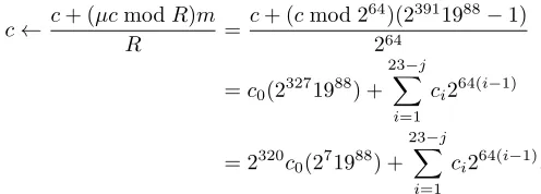
An immediate optimization based on the idea from Example1is to compute the Montgomery reduction for this particular modulus as
c←c+ (µcmodR)m
R =
c+ (cmod 264)(23723239−1) 264
=c0(23083239) + 23−j
X
i=1
ci264(i−1)
= 2256252c03239+ 23−j
X
i=1
ci264(i−1). This process is repeated 12 times (for j = 0 to 11) and
the input c is overwritten as the output for the next itera-tion. The advantage from this approach is that multiplying with 3239 < 26·64 reduces the number of multiplication
instructions (as explained in Section 3.4). The price to pay is the additional shift of52bits (the multiplication with 252). This approach lowers the number of required multiplication instruction by a factor6/7and this results in a performance increase of over five percent (see Table 4).
Finally, we implemented arithmetic modulo23911988−1:
the prime that is the result of our search for SIDH-friendly primes. The number of multiplications required is exactly the same as for the “shifting” approach but it avoids the computation of the shift operation.
c← c+ (µcmodR)m
R =
c+ (cmod 264)(23911988−1)
264
=c0(23271988) + 23−j
X
i=1
ci264(i−1)
= 2320c0(271988) + 23−j
X
i=1
ci264(i−1). Since, where the multiplication by 252 is computed using shifts, the multiplication by 2320 is a straight-forward
re-labeling of the indices of the 64-bit digits. This simplifies the code and Table 4 summarizes the reduction of the total number of instructions required for the implementation. Moreover, this immediately results in an almost12% speed-up in the modular reduction routine.
4
CURVE
ARITHMETIC
USINGADDITION-SUBTRACTION
CHAINS
The main computations in SIDH are ellitpic curve scalar multiplications of powers of 2 and p and evaluations of isogenies using V´elu’s formula [54]. In this section we inves-tigate if curve models other than Montgomery curves can be used to speed-up the elliptic curve scalar multiplication.
TABLE 5
The cost of different scalar multiplications expressed in multiplications (M) and squarings (S) inFq2as well as the number of multiplications
per bit of the scalar.
operation cost inFq2 M/bit
Montgomery triple (3) 7M+ 3S 6.78 Montgomery quintuple (5) 11M+ 7S 7.00 Montgomery septuple (7) 15M+ 9S 7.75 twisted Edwards double (2) 4M+ 4S 7.01 twisted Edwards triple (3) 10M+ 3S 7.73 twisted Edwards quantuple (5) 18M+ 8S 10.34 twisted Edwards septuple (7) 25M+ 7S 10.42
with a differential group law this is out of the scope for our investigation here. More specifically, for a fixed scalarpz
, for some integerzsuch that1≤z≤y, we search for theoptimal addition-subtraction chain (in terms of arithmetic inFq2see
Section 4.2) which can be computed using the group law on twisted Edwards curves and check if this outperforms the differential approach on using Montgomery curves. The impact on the computation of the isogenies when using this different curve model is left as future work but as outlined in [18] this computation is practical.
4.1 Outperforming Montgomery Curves?
Before starting to describe our approach to search for ef-ficient addition-subtraction chains let us take a step back and investigate if twisted Edwards curves can outperform Montgomery curves in the setting of SIDH. The extremely efficient double and triple formulas for Montgomery curves, which are used to compute elliptic curve scalar multipli-cation of 2x and 3y in practical implementations, seem hard to outperform with another curve model. In order to quantify this we ran some experiments with the opti-mized implementation of the SIKE protocol [3]: on various x86 64 architectures the ratio between the time to compute a modular squaring and a modular multiplication inFq2 is
0.75(for other ratios the discussion below can be adjusted accordingly). Table 5 summarizes the cost to compute cer-tain scalar multiples for Montgomery curves and twisted Edwards curves when using the counts given in Table 1. The cost is expressed in multiplications (in Fq2) per bit of
the scalar.
From Table 5 it becomes clear that there is indeed no hope for twisted Edwards curves to outperform Mont-gomery curves whenp∈ {3,5}. Even if one would only use twisted Edwards point doublings to compute the required bit-length the cost would be higher than repeatedly apply-ing the triple or quintuple cost for Montgomery curves.
However, motivated by our findings in Section 3, where we enhance the performance of the arithmetic in Fq2 by
selecting a modulus withp >5, and the results from [18], which show how to compute isogenies with such modi-fied moduli, we think that a systematic search for opti-mal addition-subtraction chains is an interesting alternative route to look for optimization potential for SIDH. This approach is outlined below.
4.2 Finding Addition-Subtraction Chains
To optimize the elliptic curve scalar multiplications with a prime ` > 2 the idea is to search for fast
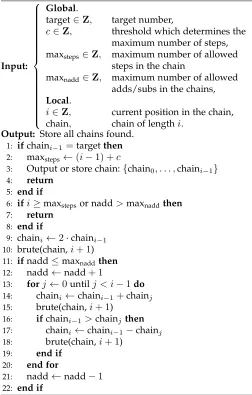
addition-Algorithm 1 Recursive approach “brute(chain,index)” to find an addition-subtraction chain with restrictions on the length and the number of additions / subtractions used.
Input:
Global.
target∈Z, target number,
c∈Z, threshold which determines the maximum number of steps, maxsteps ∈Z, maximum number of allowed
steps in the chain
maxnadd∈Z, maximum number of allowed
adds/subs in the chains,
Local.
i∈Z, current position in the chain, chain, chain of lengthi.
Output: Store all chains found.
1: ifchaini−1=targetthen
2: maxsteps←(i−1) +c
3: Output or store chain:{chain0, . . . ,chaini−1}
4: return 5: end if
6: ifi≥maxstepsor nadd>maxnaddthen 7: return
8: end if
9: chaini ←2·chaini−1
10: brute(chain,i+ 1)
11: ifnadd≤maxnaddthen 12: nadd←nadd+ 1
13: forj ←0untilj < i−1do 14: chaini←chaini−1+chainj
15: brute(chain,i+ 1)
16: ifchaini−1>chainjthen
17: chaini←chaini−1−chainj
18: brute(chain,i+ 1)
19: end if 20: end for
21: nadd←nadd−1 22: end if
subtraction chains for powers of `. The expectation is that for large scalars (e.g. larger powers of`) better chains can be found; better is measured as lowering the number of multiplications in Fq2 per bit of the scalar to compute
the various elliptic curve group operations in the addition-subtraction chain.
4.2.1 Generating Chains
The search for such addition-subtraction chains is done with a recursive algorithm which iterates over all possible chains. This approach is outlined in Algorithm 1. However, in order to speed-up this search one can set global parameters which control the maximum number of steps in the chain as well as the maximum number of additions/subtractions. The reasoning here is that most likely shorter chains, i.e. lower number of elliptic curve group operations, also result in a lower number of arithmetic operations in Fq2. The
11 TABLE 6
Overview of the best addition-subtraction chains found for usage with twisted Edwards curves (top part of the table) and the differential addition chains for usage with Montgomery curves. The cost is expressed in group operation as explained in the text and in multiplications inFq2where we
assume that the ratio between the cost of a modular squaring and a modular multiplication is0.75.
scalar chain eAp eAe pDp pDe pTp pTe #s #M #M/bits
3x 3x 0 0 0 0 x 0 1 12.25·x 7.73
51 22+ 1 1 0 1 1 0 0 2 24 10.34
52 22·3·2 + 1 1 0 2 1 1 0 2 43.25 9.31
53 (22+ 1)·22·3·2 + 5 1 1 3 2 1 0 2 68.25 9.80 54 (2·3·2 + 1)·23·3·2 + 1 2 0 4 2 2 0 2 86.5 9.31 55 ((22+ 1)·2·3·2 + 5)·23·3·2 + 5 2 1 5 1 2 0 2 111.5 9.60 56 ((25−1)·26+ 31)·23+ 1 2 1 11 3 0 0 3 129 9.26
71 3·2 + 1 1 0 0 1 1 0 2 29.25 10.42
72 23·3·2 + 1 1 0 3 1 1 0 2 50.25 8.95
73 ((23·3·2 + 1)·3·2 + 49) 1 1 3 2 2 0 2 80.5 9.56 74 (22·3·2 + 1)·24·3·2 + 1 2 0 6 2 2 0 2 100.5 8.95
111 2·3·2 + 1 1 0 1 1 1 0 2 36.25 10.48
112 (22+ 1)·22·3·2 + 1 2 0 3 2 1 0 2 67.25 9.72 113 (((26−1) + 64)·2 + 63)·22+ 63 3 1 6 3 0 0 2 103 9.92
131 2·3·2 + 1 1 0 1 1 1 0 2 36.25 9.80
132 (3·2 + 1)·22·3·2 + 1 2 0 2 2 2 0 2 72.5 9.80 133 ((24·3·2−1) + 96)·2·3·2 + 95 2 1 5 2 2 0 2 103.5 9.32
171 24+ 1 1 0 3 1 0 0 2 38 9.30
172 24·32·2 + 1 1 0 4 1 2 0 2 69.5 8.50
173 (24+ 1)·24·32·2 + 17 1 1 7 2 2 0 2 108.5 8.85
191 32·2 + 1 1 0 0 1 2 0 2 41.5 9.78
192 (22+ 1)·22·32·2 + 1 2 0 3 2 2 0 2 79.5 9.36 193 (27−1)·33·2 + 1 2 0 6 2 3 0 2 112.75 8.85 scalar chain Differential addition chains A T #s #M M/bits
3 (1·2 + 1) 0 1 2 10.75 6.78
5 (1·2 + 1) + 2 1 1 3 16.25 7.00
7 (1·2 + 1) + 1 + 3 2 1 3 21.75 7.75
11 (1·2 + 1) + 1 + 3 + 4 3 1 3 27.25 7.88
13 (1·2 + 1) + 2 + 3 + 5 3 1 3 27.25 7.36
17 (1·2 + 1) + 1 + 3 + 3 + 7 4 1 3 32.75 8.01
19 (1·2 + 1) + 2 + 2 + 5 + 7 4 1 3 32.75 7.71
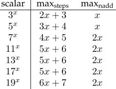
parameters as outlined in Algorithm 1. We have performed a search for various powers1 with the following starting conditions as outlined in this table.
scalar maxsteps maxnadd 3x 2x+ 3 x
5x 3x+ 4 x
7x 4x+ 5 2x
11x 5x+ 6 2x
13x 5x+ 6 2x
17x 5x+ 6 2x
19x 6x+ 7 2x
For all computations we usedc= 1to increase the threshold for the maximum number of additions / subtractions by one.
4.2.2 Arithmetic Cost of Chains
After these chains have been found we have to find the “optimal” ones. This is done by expressing the cost for the chain in arithmetic operations in Fq2 according to Table 1
and selecting the one which minimizes this cost. This is not completely trivial: since efficient triple formulas are known we have to identify, in a post-processing step, triple steps in the chains produced by Algorithm 1. This has to be done carefully since these triple formulas compute3·cas2·c+c
1. This computation is still running for different exponents, the results will be added to the final version of the paper.
but the intermediate result2·cis not directly stored: hence, if this is used in an addition later in the chain these more efficient formulas can not be applied.
To accurately compute the cost of an addition-subtraction chain it is assumed twisted Edwards curves are used together with extended twisted Edwards coordinates as outlined in Section 2.2. This means that one should be careful when to compute or omit the calculation of extended T coordinate since this has a direct impact on the arithmetic cost in Fq2. Let us write an elliptic curve operation O
as aOb where O ∈ {A,D,T} (which correspond to point addition (A), point doubling (D), and point triple (T)) and thea, b ∈ {p,e} denote of the in- or output to the elliptic curve operation is in the projective coordinate ((p), noT -coordinate) or extended coordinate system ((e), with T -coordinate). This gives the followingsixoptions in practice: eAp, eAe, pDp, pDe, pTp, and pTe. The input to the point addition is always in extended twisted Edwards form since theT-coordinate is required, however the computation of the output T-coordinate can be omitted if needed. The point double and point triple formulas do not need theT -coordinate as input.
the T-coordinate. This extended coordinate might not be immediately needed for the next step in the chain; however, when this value is later used in an point addition then this elliptic curve point should be stored together with the extended coordinate T. Hence, the situation in SIDH is different from the one in elliptic curve cryptography where in a windowing algorithm one can assume the precomputed points always are in extended form (see [29]). The usage of extended coordinates comes at a slightly higher price in SIDH. A summary of our findings is presented in Table 6. When displaying the chains the second operand to the point addition has occurred before in the computation.
4.3 Discussion of Results
As can be seen from Table 6 the cost expressed in mul-tiplication per bit of the scalar used in the elliptic curve scalar multiplication does go down when multiplying with larger scalars (i.e. addition chains for primes raised to larger exponents). In order to make an easy comparison the lower part of Table 6 shows the optimal differential chains for usage with Montgomery curves. It should be noted that the notation for the chains is slightly different compared to the upper part of the table: this is to emphasize that when adding a term the difference has occurred in the chain as well. Moreover, the notation (1·2 + 1) means the chain starts with the computation of a triple but in contrast to the twisted Edwards formula used the value2·1and 3·1 are computed and stored which means the value2can be used later.
Hence, we were not able to find any addition-subtraction chains which when used in combination with the extended twisted Edwards coordinates result in a speed-up for the el-liptic curve scalar multiplication in SIDH. When one simply applies the differential chains for the primes and applies them repeatedly to compute the scalar multiplication for higher powers using the efficient Montgomery arithmetic the result always outperforms more advanced addition-subtraction chains as far as we could verify. For larger num-bers, addition chains will become more useful for twisted Edwards curves because of the differential restriction on Montgomery curves. However, given that chains for such large numbers are difficult to find and the generally more expensive operations it is unclear if twisted Edwards curves can become faster in this setting.
5
CONCLUSIONS AND
FUTURE
WORK
We have studied various arithmetic properties which are useful for enhancing the performance in a recent post-quantum key encapsulation candidate based on the hard-ness of constructing an isogeny between two isogenous supersingular elliptic curves defined over a finite field. We have provided an overview of different techniques to compute arithmetic modulo 2xpy ±1. Although we have surveyed this in more generality it turns out that non-interleaved Montgomery reduction which is optimized for such primes is the most efficient approach in practice. Addi-tionally, we have identified other moduli suitable for SIDH which allow even faster implementations.
Furthermore, we have analyzed the relative costs of Montgomery curves, the current state-of-the-art curve type
for SIDH, and the twisted Edwards family of curves which allows precomputing more efficient addition chains. We found multiple efficient addition-subtraction chains for the scalar powers required in the key encapsulation mechanism computation. However, based on these results we have to conclude that these more efficient chains cannot compensate for the more expensive group law in twisted Edwards curves. We are still looking for more efficient addition chains and incorporating them into the computation of the isogeny tree presents an interesting challenge. The algorithm for calculating the optimal tree given by Jao and De Feo [31] cannot be easily generalized to arbitrary steps since the problem becomes much harder.
ACKNOWLEDGEMENTS
The research leading to these results has received funding from the European Union’s Horizon 2020 research and innovation programme Marie Skłodowska-Curie ITN ECRYPT-NET (Project Reference 643161) and Horizon 2020 project PQCRYPTO (Project Reference 645622). We would like to thank Michael Naehrig and Craig Costello for insightful discussions and useful comments on an early version of this paper.
REFERENCES
[1] T. Acar and D. Shumow. Modular reduction without pre-computation for special moduli. Technical report, Microsoft Re-search, 2010.
[2] D. Augot, L. Batina, D. J. Bernstein, J. W. Bos, J. Buchmann, W. Cas-tryck, O. Dunkelman, T. G ¨uneysu, S. Gueron, A. H ¨ulsing, T. Lange, M. S. E. Mohamed, C. Rechberger, P. Schwabe, N. Sendrier, F. Vercauteren, and B.-Y. Yang. Initial recommendations of long-term secure post-quantum systems, 2015. http://pqcrypto.eu. org/docs/initial-recommendations.pdf.
[3] R. Azarderakhsh, M. Campagna, C. Costello, L. D. Feo, B. Hess, A. Jalali, D. Jao, B. Koziel, B. LaMacchia, P. Longa, M. Naehrig, J. Renes, V. Soukharev, and D. Urbanik. Supersingular isogeny key encapsulation. Submission to the NIST Post-Quantum Stan-dardization project, 2017.
[4] R. Azarderakhsh, D. Fishbein, and D. Jao. Efficient implementa-tions of a quantum-resistant key-exchange protocol on embedded systems. Technical report, http://cacr.uwaterloo.ca/techreports/ 2014/cacr2014-20.pdf, 2014.
[5] P. Barrett. Implementing the Rivest Shamir and Adleman public key encryption algorithm on a standard digital signal processor. In A. M. Odlyzko, editor,CRYPTO’86, volume 263 ofLNCS, pages 311–323. Springer, Heidelberg, Aug. 1987.
[6] D. J. Bernstein, P. Birkner, M. Joye, T. Lange, and C. Peters. Twisted Edwards curves. In S. Vaudenay, editor,AFRICACRYPT 08, volume 5023 of LNCS, pages 389–405. Springer, Heidelberg, June 2008.
[7] D. J. Bernstein and T. Lange. Faster addition and doubling on elliptic curves. In K. Kurosawa, editor,ASIACRYPT 2007, volume 4833 ofLNCS, pages 29–50. Springer, Heidelberg, Dec. 2007. [8] T. Blum and C. Paar. High-radix Montgomery modular
exponenti-ation on reconfigurable hardware.IEEE Transactions on Computers, 50(7):759–764, 2001.
[9] J. W. Bos, C. Costello, H. Hisil, and K. Lauter. Fast cryptography in genus 2. In T. Johansson and P. Q. Nguyen, editors, EU-ROCRYPT 2013, volume 7881 ofLNCS, pages 194–210. Springer, Heidelberg, May 2013.
[10] J. W. Bos, C. Costello, H. Hisil, and K. Lauter. High-performance scalar multiplication using 8-dimensional GLV/GLS decomposi-tion. In G. Bertoni and J.-S. Coron, editors,CHES 2013, volume 8086 ofLNCS, pages 331–348. Springer, Heidelberg, Aug. 2013. [11] J. W. Bos and S. Friedberger. Fast arithmetic modulo 2ˆ xpˆ y±1. In