Three-term backpropagation algorithm for classification problem

(1)

THREE-TERM BACKPROPAGATION ALGORITHM FOR CLASSIFICATION PROBLEM

FADHLINA IZZAH BINTI SAMAN

A project report submitted in partial fulfillment of the requirements for the award of the degree of

Master of Science (Computer Science)

Faculty of Computer Science and Information System Universiti Teknologi Malaysia

(2)

(3)

iv

ACKNOWLEDGEMENT

In the name of Allah, Most Merciful, Most Compassionate. It is by God’s willing, I was able to complete this project within the time given. This project would not have been possible without the support of many people. Firstly, I would like to take this opportunity to thank my supervisor, Associate Professor Dr. Siti Mariyam bt. Shamsuddin for her guidance, patience and support for me throughout the period of time in doing this project. I also would like to thank Dr. Siti Zaiton Mohd. Hashim as my co-supervisor for her valuable comments and suggestions to further improve my analysis and writing. My deepest gratitude also goes out to my examiners, Dr. Ali Selamat and Dr. Norazah Yusof for their constructive comments and suggestions in evaluating my project.

(4)

ABSTRAK

(5)

vi

ABSTRACT

(6)

TABLE OF CONTENT

CHAPTER TITLE PAGE

TITLE i

DECLARATION ii

DEDICATION iii

ACKNOWLEDGEMENT iv

ABSTRAK v

ABSTRACT vi

TABLE OF CONTENT vii

LIST OF TABLES x

LIST OF FIGURES xii

LIST OF SYMBOLS xiii

LIST OF ABBREVIATION xiv

LIST OF APPENDICES xv

1 INTRODUCTION 1

1.1 Introduction 1

1.2 Problem Background 2

1.3 Problem Statement 5

1.4 Project Aim 5

1.5 Project Objectives 6

1.6 Project Scopes 6

1.7 Significance of The Project 7

1.8 Project Plan 7

(7)

viii

2 LITERATURE REVIEW 9

2.1 Introduction 9

2.2 Artificial Neural Network 10

2.3 Standard Backpropagation Algorithm 13

2.3.1 BP Learning 13

2.3.2 Two term parameters 15

2.4 Three-Term Backpropagation Algorithm 17

2.5 Summary 20

3 METHODOLOGY 21

3.1 Introduction 21

3.2 Dataset 24

3.2.1 Balloon Dataset 24

3.2.2 Iris Dataset 25

3.2.3 Cancer Dataset 26

3.3 Defining Neural Network Architecture 26

3.3.1 Balloon Dataset 27

3.3.3 Iris Dataset 28

3.3.3 Cancer Dataset 30

3.4 Training BP Algorithm 31

3.5 Implementing Proportional Factor, γ 32 3.6 Comparing Standard and Three-Term BP 36

3.7 Experiment and Analysis 37

3.8 Summary 37

4 RESULT 38

4.1 Introduction 38

4.2 Experimental Result 39

4.2.1 Balloon Dataset Analysis 40

4.2.2 Iris Dataset Analysis 44

(8)

Algorithm

4.4 Stability Analysis 55

4.5 Discussion 59

4.6 Summary 61

5 CONCLUSION AND FUTURE WORK 62

5.1 Introduction 62

5.2 Summary of Work 63

5.3 Conclusion 64

5.4 Suggestion for Future Works 65

REFERENCES 66

(9)

x

LIST OF TABLES

TABLE NO TITLE PAGE 1.1 List of few approaches in improving BP performance 4

2.1 Behaviour of α 16

2.2 Characteristics of BP Learning Parameters 19 3.1 Summary of Balloon Attributes for Classification 25 3.2 Summary of Iris Attributes for Classification 25 3.3 Summary of Iris Attributes for Classification 26

3.4 Network Architecture for Balloon Dataset 28

3.5 Network Architecture for Iris Dataset 29

3.6 Network Architecture for Cancer Dataset 30

(10)

4.7 Percentage of correct classification for standard and Three-Term BP

54

4.8 Eigen Values for Iris and Cancer Dataset 58

(11)

xii

LIST OF FIGURES

FIGURE NO TITLE PAGE

2.1 MLP Architecture 12

3.1 A General Framework of the Study 23

3.2 Network Structure for Balloon Dataset 28

3.3 Network Structure for Iris Dataset 29

3.4 Network Structure for Cancer Dataset 31

4.1 Characteristic Convergence of Balloon Dataset 43 4.2 Characteristic Convergence of Iris Dataset 47 4.3 Characteristic Convergence of Cancer Dataset 51 4.4 Convergence comparison between standard and

Three-Term BP

53

4.5 Comparison of correct classification between standard and Three-Term BP

54

(12)

LIST OF SYMBOLS

ij

W - Weight connected between node i and j i

θ - Bias of node i

j

O - Output of node j

) (t

W_ij - Weight from node i to node j at time t, ij

W

∆ - Weight adjustment

α - Learning rate

β - Momentum term

γ - Proportional factor

j

δ - Error signal at node j

j

T - Target output value at node j j

O - Actual output of the network at node j

tkj - Target value from output node (k) to hidden node (j) okj - Network value from output node (k) to hidden node (j) Ek - Error at output unit k

m - Number of input nodes

n - Number output nodes

(13)

xiv

LIST OF ABBREVIATION

ANN - Artificial Neural Network

BP - Backpropagation

MLP - Multilayer Perceptron

MSE - Mean Squared Error

(14)

LIST OF APPENDICES

APPENDIX TITLE PAGE

A Results of standard and Three-Term BP using small scale data (Iris and Cancer dataset)

(15)

CHAPTER 1

INTRODUCTION

1.1 Introduction

Classification can be defined as deciding the category or grouping to which an input value belongs (Ishbushi et al., 1999). Classification is defining a set of groups by their characteristics, then each case is analyzed and put it into the group it belongs. Classification can be used to understand the existing data and to predict how new instances will behave. The goal of data classification is to organize and categorize data in distinct classes. A model is first created based on the data distribution. The model is then used to classify new data. Given the model, a class can be predicted for new data.

(16)

The BP algorithm involves backward error correction of the network weights. Training is usually done by weights updating iteratively using a mean-square error function. Traditionally, the standard BP algorithm utilizes two terms parameters called Learning Rate (α) and momentum factor (β) for weight adjustment.

1.2 Problem Background

BP algorithm is a widely used learning algorithm in NN. Despite the general success of the BP algorithm, there are several drawbacks and limitations that still exist (Zweiri et al., 2003). Limitations of standard BP:

1 The existence of temporary, local minima resulting from the saturation behaviour of the activation function.

2 The slow rates of convergence. Convergence rate is relatively slow for network with more than one hidden layer.

3 Some of the modification of BP algorithm requires complex and costly calculations at each iteration, which offset their faster rates of convergence.

(17)

3

Kim et al. (2004) has used Genetic Algorithm (GA) to determine learning rate and momentum parameter. Although GA is proven to give better performance than the standard BP which uses trial and error method to obtain the learning rate and momentum, but is changes the structure of the BP computation. Jia and Yang (1993) proposed an improved algorithm with stochastic attenuation momentum factor. Compared with the standard BP algorithm, the algorithm claims to effectively cancel the negative effect on momentum of network. However, the computation of this proposed approach is complex since it uses the correlation matrix in defining the momentum. Roy (1994) proposed a new method to compute dynamically the optimal learning rate. By using this method, a range of good static learning rates could be found. Although this method could improve the performance of standard BP, the algorithm is computationally complex and might take longer to train than standard BP. Yu and Chen (1996) proposed a BP algorithm using dynamically optimal learning rate and momentum factor. This approach claims to have remarkable savings in running time. However, this approach also its disadvantages of having complex computation and storage burden for estimating the optimal learning rate and momentum factor at most triple that of the standard BP.

(18)

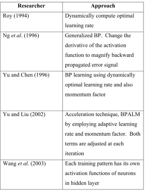
Table 1.1 : List of few approaches in improving BP performance

Researcher Approach Roy (1994) Dynamically compute optimal

learning rate

Ng et al. (1996) Generalized BP. Change the derivative of the activation function to magnify backward propagated error signal

Yu and Chen (1996) BP learning using dynamically optimal learning rate and also momentum factor

Yu and Liu (2002) Acceleration technique, BPALM by employing adaptive learning rate and momentum factor. Both terms are adjusted at each iteration

Wang et al. (2003) Each training pattern has its own activation functions of neurons in hidden layer

The standard BP algorithm usually uses two parameters which are Learning Rate (α) and Momentum Factor, (β) for controlling the weight adjustment of the ANN. Zweiri et al. (2003) proposes an additional term, proportional factor (γ) for BP learning. In this study, a new term γ of Zweiri et al, (2003) will be implemented in addition of the existing terms ά and β. to calculate the change of weight for BP learning enhancement

(19)

5

third term is done with the hope of improving and speeding the BP learning without having to change the BP structure into a more complex structure. It maintains the computation complexity of standard BP as it is, since γ is added in the formulation of network’s weight adaptation.

1.3 Problem Statement

Although the standard BP provides a solution to the problem of learning in multilayer networks, it also has its own weaknesses and limitations. The BP learning can be improved by selection of better activation function and optimal learning parameters which are learning rate and momentum values (Ng et al., 1996). This study will focus on learning parameters by adding a third term which is the proportional factor, γ. The γ factor will be implemented in the network weight adjustment to test its efficiency.

Therefore, the hypothesis of this study can be stated as:

How efficient is the Proportional Factor,γ in Three-Term BP compared to Standard BP in terms of the convergence speed and classification accuracy?

1.4 Project Aim

(20)

Three-Term and Standard BP is carried out. These algorithms will be used to solve classification problem using universal data which are Balloon, Iris and Cancer dataset. Various values of α, β and γ will be experimented to search for better parameters tuning for Three-Term BP.

1.5 Project Objectives

The objectives of the study are defined as follows:

1. To investigate the efficiency of Proportional Factor, γ of Three-Term BP in classification problem.

2. To compare the performance between standard BP and Three-Term BP.

1.6 Project Scopes

The project scopes are defined as follows:

1. Balloon, Iris and Cancer dataset will be used as the training and testing data set which represent small, medium and large scale data.

(21)

7

1.7 Significance of Project

This project will investigate the performance of Three-Term BP proposed by Zweiri et al. (2003), by comparing it with Standard BP. The evaluation will be carried out since there is no extensive comparison between Standard BP and Three-Term BP has been done before and to see whether it can give better convergence rate for BP learning or not. The results of this study can be used to verify the efficiency of Three-Term BP and will contribute in future works for BP improvement.

1.8 Project Plan

This project will be carried out in two semesters. The first part of the project is done in the first semester where the understandings of literature review and methodology that will be used are done. Gathering information about the study is a crucial part of this part since thorough understanding is needed in order to really implement the proposed approach. Most of the information is obtained from articles and journal that can be downloaded from the Institute of Electrical and Electronic Engineering (IEEE) website and ScienceDirect website. The second part of the project is to implement the Three-Term BP and analyze the results with standard BP.

1.9 Organization of the Report

(22)

(23)

CHAPTER 2

LITERATURE REVIEW

Backpropagation (BP) algorithm is a supervised learning technique used for training Multi-Layer Perceptrons (MLPs). BP is used to calculate the gradient of the error of the network with respect to the network's modifiable weights. The BP algorithm attempts to minimize the difference (or error) between the desired and actual outputs in an iterative manner. For each iteration, the weights involved in the network are adjusted by the algorithm to make the error decrease along a descent direction (Yu and Chen, 1997).

(24)

et al, 1995). Another drawback of standard BP is the existence of local minima resulting from the saturation behaviour of the activation function (Zweiri et al., 2003). Many researches had been done in order to improve the performance of standard BP algorithm. However, the algorithm modification usually involves complex calculations at each iteration.

Zweiri et al. (2003) had proposed a third term, which is the Proportional Factor to overcome the problems of Standard BP. The algorithm, Three-Term BP has never been implemented before in terms of programming. Thus, this project is carried out mainly to investigate the performance of Three-Term BP and compare it with Standard BP.

2.2 Artificial Neural Network

Artificial Neural Network (ANN) is an interconnected group of artificial neurons that uses a mathematical or computational model for information processing based on a connectionist approach to computation.

(25)

11

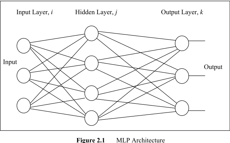
ANN can be classified as either feedforward, recurrent, modular, stochastic and many others, depending on how data is processed through the network. The feedforward neural networks are the first and simplest type of neural networks. In this network, the information moves in only one direction which is forward from the input nodes, through the hidden nodes and to the output nodes. The connections are formed by connecting each of the nodes in a given layer to all of the neurons in the next layer. In this way every node in a given layer is connected to every other node in the next layer.

Usually there are at least three layers (Yam and Chow, 1999) to a feedforward network which are an input layer, a hidden layer, and an output layer. The input layer does no processing. It is where the data is fed into the network. The input layer then feeds into the hidden layer. The hidden layer, in turn, feeds into the output layer. The actual processing in the network occurs in the nodes of the hidden layer and the output layer.

When enough neurons are connected together in layers, the network can be trained to do useful things using a training algorithm. Feedforward networks usually can be trained to do classification or identification type tasks on unfamiliar data.

Another way of classifying ANN types is by their method of learning, as some ANN employs supervised learning while others are referred to as unsupervised or self-organizing. Supervised learning is a learning process where both the input and outputs are provided. Unsupervised learning is a learning process where the network is provided with inputs but not with desired outputs.

(26)

historical data so that the model can then be used to produce the output when the desired output is unknown. A graphical representation of an MLP is shown in Figure 2.1.

ANN is used to train input data so that it can generate the appropriate output according to the desired target. Before the training process starts, all weights must be initialized to small random numbers. This is to make sure that the network is not saturated by large values of the weights. The process of training an ANN is based on five steps (Auda et al., 1990). The steps are as follows:

1. Select the training pair from training set, applying the input vector to the network input

2. Calculate the output of the network.

3. Calculate the error between the network output and the desired output. 4. Adjust the weights of the network in a way that minimizes the error. 5. Repeat step 1 through 4 until the error is acceptably low.

Input Layer, i Hidden Layer, j Output Layer, k

Input

Output

(27)

13

2.3 Standard Backpropagation Algorithm

The BP algorithm is one of the most popular methods in training MLPs. There are two relatively standard definitions of backpropagation (Fogel et al., 2003). The first defines backpropagation as a procedure for efficiently calculating the derivatives of some function of the outputs of any nonlinear differentiable system, with respect to all inputs and parameters of that system, through calculations proceeding backwards from outputs to inputs. The second standard definition of backpropagation is any technique for adapting the weights or parameters of a nonlinear system by using such derivatives or equivalent.

Network size usually refers to the number of hidden layers and of neurons in each layer. The network size is a compromise between generalization and convergence. Convergence is the capacity of the network to learn the patterns on the training set and generalization is the capacity to respond correctly to new patterns. The best way is to implement the smallest network possible, so it is able to learn all patterns and, at the same time, provide good generalization (Yu et al., 1997).

2.3.1 BP Learning

(28)

The output for j th layer is given by

j i j

ji

j W O

net f

Output= ( )=

∑

+θ where,

Wji is the weight connected between node i and j, j

θ

is the bias of node i,

i

O is the output of node j.

The most common activation function of a neuron f(x) is sigmoid function (Wang et al, 2003) as shown below:

) 1 ( 1 ) ( j net j e net f ₋ + =

In the second phase, the errors calculated in the output layer are then back propagated to the hidden layers where the synaptic weights are updated to reduce the error. This learning process is repeated until the output error value, for all patterns in the training set, are below a specified value.

(29)

15

2

1

) (

2 1

pj N

j pj

p t o

E =

∑

−

=

where, p

E = error for the p th presentation vector

tkj is the desired value from output node (k) to hidden node (j) okj is the network value from output node (k) to hidden node (j)

The weight adaptation in standard BP is defined as:

( )

=

(

−

) (

1−

)

+ ∆

(

−1

)

∆W_kj n α t_k o_k o_k o_k O_j β W_kj n

From equation above, we could see that there are two terms added to the equation which are the α and β. These are the two terms that are usually utilized in standard BP or also known as two-term BP. The terms are added for reasons that will be stated in next section.

2.3.2 Two Term Parameters

The learning rate parameter (α) is used to determine how fast the BP method converges to the minimum solution. In the conventional BP learning rule, α is a decisive factor in regard to the size of weights adjustments made at each iteration and therefore it affects the convergence rate. In standard BP, α is constant throughout the training. The BP performance is very sensitive to the proper setting of the α term.

(30)

( )

(

k k

) (

k k

)

j

)

kj

n

t

o

O

W

=

−

∆

α

1

(2.1)

The best choice of α depends on problem and needs trial and error before a good choice is found. According to Yu and Liu (2002) the larger the learning rate, the bigger the step and the faster the convergence. However, if the α value is made too large the algorithm will become unstable. On the other hand, if the α value is set to too small, the algorithm will take a long time to converge. According to Sexton and Gupta (2000), if the α value is too small, it will lead to slow convergence. If the α value is too big, oscillation and overshooting of minimum will occur. The summary for behaviour of α are shown in Table 2.1.

Table 2.1 : Behaviour of α

Value Effect Small • Slow convergence

Big • Bigger steps • Faster convergence

• Oscillation and overshooting of minimum if α value too big

(31)

17

output is reduced. By using β in weight adaptation, a larger learning rate can be used while maintaining the stability of the algorithm. β also tends to accelerate convergence. The weight adaptation equation from kth layer to the jth layer with both α and β terms is written as follows:

( )

=

(

−

) (

1−

)

+ ∆

(

−1

)

∆W_kj n α t_k o_k o_k o_k O_j β W_kj n (2.1) where,

β is proportional to the previous value of the incremental change of the weights

The advantages of using β term can be summarized as follows: 1. Might smooth out oscillations occur in learning

2. Larger α value can be used if β is added in weight adaptation calculation 3. Encourages movement in the same direction of successive steps

2.4 Three-Term Backpropagation Algorithm

(32)

even if the output error is large, leading to very little progress in the weight adjustment.

This study will focus on the implementation of Three-Term BP. The standard BP weight adaptation equation given by (2.1)is modified by adding an extra term in order to increase the BP learning speed. The modification is done by adding a third term proposed by Zweiri et al. (2003). The third term, being the proportional term (γ)γ is proportional to:

e(W(k)) = es

where,

es represents the difference between the output and target at

each iteration

Hence the new weight adaptation for three-term BP is defined as follows:

( )

k

(

E

(

W

( )

k

)

W

(

k

)

e

(

W

( )

k

)

W =α −∇ +β∆ − +γ

∆ 1 (2.2)

where,

α is proportional to the derivative of E (W(k)),

β is proportional to the previous value of the incremental change of the weights,

γ is proportional to es

From equation (2.2), E(W(k)) can also be written as j O

k

E(W(k))=δ (2.3)

Also from equation (2.2), for batch learning, e(W(k)) could be written as

[

]

τ

s s se e e k W

e( ( ))= ... where,

vector e is of appropriate dimension of τ,

and,

[

Tj −Oj

]

=

s

(33)

19

where,

es represents the difference between the output and the target

at each iteration.

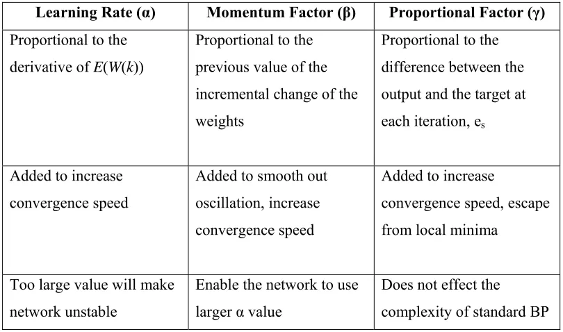
Some of the modifications of BP algorithms require complex and costly calculations at each iteration, which will only offset the faster rates of convergence that is obtained using the modified BP algorithms. As we can see from equation (2.2), the Three-Term BP will maintain the simplicity of standard BP algorithm. In the paper by Zweiri et al. (2003), Three-Term BP was tested on XOR problem and it had significantly increased the convergence speeds while maintaining the simplicity and efficiency of standard BP. the characteristics of each learning parameters in Three-Term BP is summarized in Table 2.2.

Table 2.2 : Characteristics of BP Learning Parameters

Learning Rate (α) Momentum Factor (β) Proportional Factor (γ) Proportional to the

derivative of E(W(k))

Proportional to the previous value of the incremental change of the weights

Proportional to the difference between the output and the target at each iteration, es

Added to increase convergence speed

Added to smooth out oscillation, increase convergence speed

Added to increase

convergence speed, escape from local minima

Too large value will make network unstable

Enable the network to use larger α value

Does not effect the

(34)

2.5 Summary

(35)

CHAPTER 3

METHODOLOGY

This chapter discusses the methodology that will be used in this project and describes the techniques and parameters that are required in BP learning. The next section will discuss the experiments and analysis of results in order to investigate the efficiency of Three-Term BP. A comparison between standard BP and Three-Term BP in solving classification problems is also addressed.

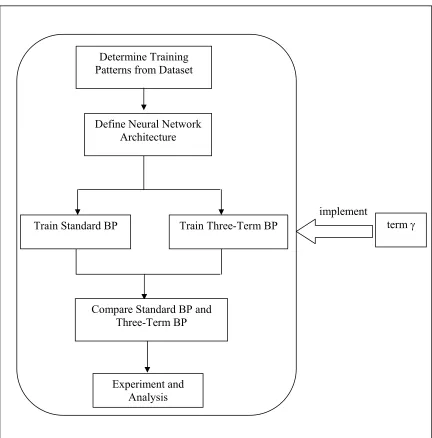
There are a few basic steps in order to implement the standard BP. These basic steps will also be used in implementing the Three-Term BP. The basic steps could be defined as follows:

1. Determine training patterns from dataset 2. Define neural network architecture 3. Start training standard BP

(36)

5. Train Three-Term BP

6. Do comparison of standard BP and three term BP 7. Experiment and analysis

(37)

23

Figure 3.1 A General Framework of the Study Determine Training

Patterns from Dataset

Define Neural Network Architecture

Train Standard BP Train Three-Term BP term γ

Experiment and Analysis

Compare Standard BP and Three-Term BP

(38)

3.2 Dataset

The dataset used in solving classification problem using BP algorithm are Balloon dataset, Iris dataset and Cancer dataset. These data represents small, medium and large scale data based on their size. Balloon data is chosen to represent small scale data, Iris data represents medium scale data and Cancer data represents large scale data. These data are used to evaluate the performance of both standard and Three-Term BP algorithms in terms of classification accuracy and convergence speed.

3.2.1 Balloon Dataset

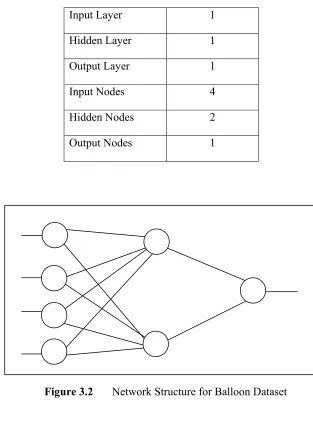
Balloon dataset is used to represent small scale data. It is used for classifying four balloon attributes which are colour (yellow, purple), size (large, small), act (stretch, dip) and age (adult, child) into a class, either inflated (T) or not (F). Balloons dataset contains 16 instances. The network will have 4 inputs to represent information for each attribute and 1 output to represent either it is inflated or not. The Balloon dataset were split with 12 for training data and 4 for testing data, totalling 16 instances for the whole Balloon dataset.

There are four sets of data in Balloons dataset that represents different conditions of an experiment which are:

1. Adult-stretch data: Inflated is true if age = adult or act = stretch 2. Adult + stretch data: Inflated is true if age = adult and act = stretch

3. Small - yellow data: Inflated is true if (colour = yellow and size = small) or 4. Small – yellow + adult – stretch data: Inflated is true if (colour = yellow

(39)

25

The summary for Balloon dataset for classification is shown in Table 3.1 below:

Table 3.1 : Summary of Balloon Attributes for Classification

No. Attribute Value1 Value2

1 Colour Yellow Purple

2 Size Large Small

3 Act Stretch Dip

4 Age Adult Child

3.2.2 Iris Dataset

The classifying of Iris dataset involves classifying the data of petal width, petal length, sepal width and sepal length into three classes of species which are iris Setosa, Versicolor and Verginica. This dataset contains data for the three classes with 25 instances for each class. The input consists of 4 numeric attributes related to the length and the width of the sepals and petals of iris plant. The network will have 4 inputs and 3 outputs to separate the pattern. Summary of Iris dataset attributes for classification is shown in Table 3.2.

Table 3.2 : Summary of Iris Attributes for Classification No. Attribute Value

1 Petal Width 2 Petal Length 3 Sepal Width 4 Sepal Length

(40)

3.2.3 Cancer Dataset

The classifying of Cancer dataset involves classifying the data into two classes of breast lump’s diagnosis which are either benign or malignant. These data were obtained from automated microscopic examination of cells collected by needle aspiration. All inputs are continuous variables and 65.5% of the examples are benign. The data set was originally generated at hospitals at the University of Wisconsin Madison, by Dr. William H. Wolberg. The data set includes 9 inputs and 1 output. The data are split into 500 for training, and 100 for testing, totaling of 600 instances. Summary of Cancer dataset attributes for classification is shown in Table 3.3.

Table 3.3 : Summary of Cancer Attributes for Classification No. of Instances

Training 500

Testing 100

Total of Instances 600

3.3 Defining Neural Network Architecture

(41)

27

project, the network architecture is defined as to solve to classification problem for Balloon, Iris and Cancer data.

The number of nodes required in each layer differs from one dataset to another. Each input node defined represents the set of problem that will be classified and the output node represents the classes that the input data will belong to after classification has been done. The number of hidden nodes will be defined as (Masters, 1993):

number of hidden nodes= m* n where,

m is the number of input nodes, n is number output nodes

The summary of defined neural network architecture for this project is shown according to dataset.

3.3.1 Balloon Dataset

(42)

Table 3.4 : Network Architecture For Balloon Dataset

Input Layer 1

Hidden Layer 1

Output Layer 1

Input Nodes 4

Hidden Nodes 2

Output Nodes 1

3.3.2 Iris Dataset

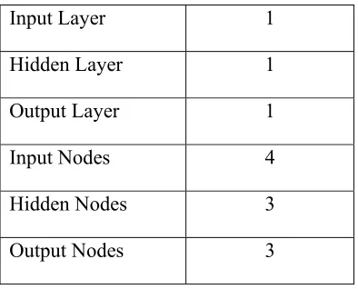
The network architecture for Iris dataset comprises of 4 input nodes, 3 output nodes and 3 hidden nodes. The Iris dataset has 4 attributes for each instances of Iris which are the petal width, petal length, sepal width and sepal length. This is why 4 input nodes are chosen to represent this problem. Meanwhile, for the selection of the output nodes are based on the 3 types of Iris that each instances will be classified into which are Setosa, Versicolor and Verginica. Therefore, the number of output nodes

(43)

29

chosen for this problem is 3. The complete summary of the network architecture used in representing this problem can be viewed in Table 3.5. The network structure for this dataset is shown is Figure 3.3.

Table 3.5 : Network Architecture For Iris Dataset

Input Layer 1

Hidden Layer 1

Output Layer 1

Input Nodes 4

Hidden Nodes 3

Output Nodes 3

(44)

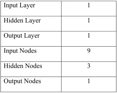
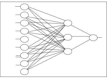
The network architecture for Cancer dataset comprises of 9 input nodes, 1 output nodes and 3 hidden nodes. The Cancer dataset has 9 attributes for each instances of Cancer. This is why 9 input nodes are chosen to represent this problem. Meanwhile, for the selection of the output node is based on the one output class which is type of Cancer. Therefore, the number of output node chosen for this problem is 1 node. The value for this class is either benign or malignant type of breast cancer diagnosis. The complete summary of the network architecture used in representing this problem can be viewed in Table 3.6. The network structure for this dataset is shown is Figure 3.4.

Table 3.6 : Network Architecture For Cancer Dataset

Input Layer 1

Hidden Layer 1

Output Layer 1

Input Nodes 9

Hidden Nodes 3

(45)

31

3.4 Training BP algorithm

The standard BP needs to be trained to minimize the error measure by adjusting the weights. The network will be trained after all the network structures have been defined. In order to train the network, the initial weights and bias must be defined. Another parameter that is needed to be defined is the activation function. This project will use sigmoid function as an activation function. The maximum error must also be defined as it would be used as comparison with the network error and the training will be repeated until the network error is less than maximum error.

The basic steps in training BP are as follows:

1. Apply input to the network. 2. Calculate the output.

(46)

3. Compare the resulting output with the desired output for the given input. This is called the error.

4. Modify the weights and threshold θ for all neurons using the error. 5. Repeat the process until error reaches an acceptable value which

means that the NN was trained successfully, or if a maximum count of iterations is reached, then it means the NN training was not successful.

The same steps will also be used to train Three-Term BP. The difference between standard BP and Three-Term BP is in terms of the weight adjustments, and will be discussed in next section.

3.5 Implementing Proportional Factor, γ

The standard BP usually utilizes two term which are the learning rate, α and momentum factor, β.The proportional factor, γ will be implemented in Three-Term BP alongside the other two terms α and β. The value of γ will be determined using trial and error method.

(47)

33

The error measure, E used in this project is the Mean Square Error (MSE). E is defined as follows:

2 1 ) ( 2 1 kj N j kj

p t o

E =

∑

−

=

where, p

E = error for the pth presentation vector

tkj is the desired value from output node (k) to hidden node (j) okj is the network value from output node (k) to hidden node (j)

The weight changes are proportional to the derivative of E. For example, the change in weights between output layer, k and hidden layer, j can be written as follows: kj kj W E W ∂ ∂ − = ∆ α where,

α

is learning rate

By chain rule, equation above can be written as:

kj k k kj W net net E W E ∂ ∂ × ∂ ∂ = ∂

∂ _(3.1)

Let the error signal, δk be

k k net E ∂ ∂ =

δ (3.2)

Since _k

k j kj

k W O

net =

∑

+θ ,by doing a partial derivation of it we will get

kj k j W net O ∂ ∂

(48)

By substituting (3.3) and (3.2) into (3.1), we will get j k kj O W

E ₌ _× ∂

∂ _δ

(3.4)

From (3.2), we know that

k k net E ∂ ∂ = δ .

This is obtained by chain rule

k k k k net o o E ∂ ∂ × ∂ ∂ =

δ (3.5)

The partial derivative of error function, 1 ₍ ₎2

2 kj kj

k

E=

∑

t −o can be written as

(

k k

)

k

o t o

E ₌₋ ₋ ∂

∂

(3.6)

The output of k th layer is given by

k net k e o ₋ + = 1 1 .

Therefore the partial derivative of ok is written as

(

k

)

k k

k _o _o

net o − = ∂ ∂

1 (3.7)

By substituting (3.6) and (3.7) into (3.5), we will get

(

k k

) (

k k

)

k =− t −o o 1−o

δ (3.8)

By substituting (3.8) into (3.4), we will get

(

k k

) (

k k

)

j kj O o o o t W E × − − − = ∂ ∂

(49)

35

The weight adaptation between output layer and hidden layer now can be written as

kj kj W E W ∂ ∂ − =

∆ α (3.10)

By substituting (3.9) into (3.10), we will get

( )

(

k k

) (

k k

)

j

)

kj

n

t

o

O

W

=

−

∆

α

1 ( )

(

k k

) (

k k

)

j

kj n t o o o O

W = − −

∆ α 1 (3.11)

By adding momentum term

β

to equation (3.11), the weight adaptation is now

( )

=

(

−

) (

1−

)

+ ∆

(

−1

)

∆W_kj n α t_k o_k o_k o_k O_j β W_kj n (3.12)

γ factor is added to equation (3.12) giving the weight adaptation as

( )

k

(

E

(

W

( )

k

)

W

(

k

)

e

(

W

( )

k

)

W =α −∇ +β∆ − +γ

∆ 1 (3.13)

where,

α is proportional to the derivative of E(W(k)),

β is proportional to the previous value of the incremental change of the weights,

γ is proportional to es

From equation (3.13), E(W(k)) can also be written as j O

k

E(W(k))=δ (3.14)

where,

k

(50)

Also from equation (3.13), for batch learning, e(W(k)) could be written as

[

]

τ

s s se e e k W

e( ( ))= ... where,

vector e is of appropriate dimension of τ,

and, e_s =

[

T_j−O_j

]

where,

es represents the difference between the output and the target

at each iteration.

The weights adaptation between hidden layer , j and input layer, i of the standard BP algorithm is similar as updating weight between output layer, k and hidden layer, j (Ng et al., 1996).

3.6 Comparing Standard and Three-Term BP

(51)

37

3.7 Experiment and Analysis

The experiment and analysis part must be carried out in this project to achieve one of its objectives which is to evaluate the performance of Three-Term BP and do a comparative study between the standard and Three-Term BP in terms of performance, after using the same value for the network parameters for both standard and Three-Term BP.

The analysis part will be done in testing the network of standard and Three-Term BP. The testing is done to evaluate the performance of the Three-Three-Term BP algorithm in solving the classification problem.

3.8 Summary

This chapter discusses mainly about the methodology that will be used throughout this project. The basic steps in the methodology are discussed and a general framework of the study is also shown in this chapter.

(52)

CHAPTER 4

EXPERIMENTAL RESULTS AND ANALYSIS

This chapter discusses the experimental results of this project and its analysis. The experimental results are obtained from training both the standard and Three Term BP. The results are measured from its performance in terms of convergence rate and classification accuracy of the Balloon, Iris and Cancer dataset.

(53)

39

scale data. The analysis of both standard and Three-Term BP’s performance will be discussed in next section.

4.2 Experimental Result

Balloon, Iris and Cancer data were used for training and testing the standard and Three-Term BP throughout this project. For standard BP, the experiments are divided into two set of tests which contains 9 trials each. For the first test (Test I), the same value of α and β are used in the range of [0.1, 0.9]. While in the second test (test II), the values of α and β are increased and decreased, respectively with 0.1 as the initial value for α and 0.9 for β.

For Three-Term BP, the experiments are divided into three set of tests which also contains 9 trials each. For the comparisons, Three-Term BP uses the same value range of α, β and γ which is also [0.1, 0.9]. The first test (Test I) uses the same values of α, β and γ for all 9 trials. The second test (Test II) uses the same increasing value for α and β and decreasing value for γ. α and β values start from 0.1 and γ value starts from 0.9. The third test (Test III) uses increasing value for α and decreasing values for both β and γ, where α value starts from 0.1 and β and γ values both start from 0.9.

(54)

4.2.1 Balloon Dataset Analysis

Balloon dataset are used to represent small scale data where the data consists of 16 instances. In Balloon dataset experiment, the network architecture consists of 4 input nodes, 2 hidden nodes and 1 output node. 12 instances were represented to the network as training data set and 4 instances as testing data set. The results of Standard BP are shown in Table 4.1(a) and (b), while for Three-Term BP, the results are shown in Table 4.2(a), (b) and (c).

Table 4.1(a) : Results of Standard BP in Balloon Dataset (Test I)

TE1 TE2 TE3 TE4 TE5 TE6 TE7 TE8 TE9 Learning

Rate 0.1 0.2 0.3 0.4 0.5 0.6 0.7 0.8 0.9

Momentum 0.1 0.2 0.3 0.4 0.5 0.6 0.7 0.8 0.9

Error

Generated 0.04993 0.0499 0.0497 0.0497 0.0492 0.0495 0.0481 0.0497 0.0493 Learning

Iteration 1041 455 261 164 107 69 44 28 25

Process Time 1.000 0.001 0.001 0.001 0.001 0.001 0.001 0.001 0.001

Correct

Classification 75% 75% 75% 75% 75% 75% 75% 75% 75%

Table 4.1(b) : Results of Standard BP in Balloon Dataset (Test II)

TE1 TE2 TE3 TE4 TE5 TE6 TE7 TE8 TE9

Learning Rate 0.1 0.2 0.3 0.4 0.5 0.6 0.7 0.8 0.9

Momentum 0.9 0.8 0.7 0.6 0.5 0.4 0.3 0.2 0.1

Error

Iteration 115 112 110 108 107 106 105 105 105

Process Time 0.001 0.001 0.001 0.001 0.001 0.001 0.001 0.001 0.001

Correct

(55)

41

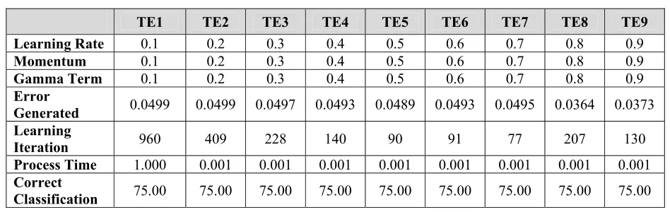
Table 4.2(a) : Results of Three-Term BP in Balloon Dataset (Test I)

Learning Rate 0.1 0.2 0.3 0.4 0.5 0.6 0.7 0.8 0.9

Momentum 0.1 0.2 0.3 0.4 0.5 0.6 0.7 0.8 0.9

Gamma Term 0.1 0.2 0.3 0.4 0.5 0.6 0.7 0.8 0.9

Error

Iteration 960 409 228 140 90 91 77 207 130

Process Time 1.000 0.001 0.001 0.001 0.001 0.001 0.001 0.001 0.001

Correct

Classification 75.00 75.00 75.00 75.00 75.00 75.00 75.00 75.00 75.00

Table 4.2(b) : Results of Three-Term BP in Balloon Dataset (Test II)

TE1 TE2 TE3 TE4 TE5 TE6 TE7 TE8 TE9 Learning Rate 0.1 0.2 0.3 0.4 0.5 0.6 0.7 0.8 0.9

Momentum 0.1 0.2 0.3 0.4 0.5 0.6 0.7 0.8 0.9

Gamma Term 0.9 0.8 0.7 0.6 0.5 0.4 0.3 0.2 0.1

Error

Iteration 1136 485 233 136 90 62 44 35 23

Process Time 1.000 0.001 0.001 0.001 0.001 0.001 0.001 0.001 0.001

Correct

Classification 75.00% 75.00% 75.00% 75.00% 75.00% 75.00% 75.00% 75.00% 75.00%

Table 4.2(c) : Results of Three-Term BP in Balloon Dataset (Test III)

Learning Rate 0.1 0.2 0.3 0.4 0.5 0.6 0.7 0.8 0.9

Momentum 0.9 0.8 0.7 0.6 0.5 0.4 0.3 0.2 0.1

Gamma Term 0.9 0.8 0.7 0.6 0.5 0.4 0.3 0.2 0.1

Error

Iteration 168 147 115 97 90 91 92 100 107

Process Time 0.001 0.001 0.001 0.001 0.001 0.001 0.001 0.001 0.001

Correct

Classification 75.00% 75.00% 75.00% 75.00% 75.00% 75.00% 75.00% 75.00% 75.00%

(56)

(57)

43

Figure 4.1 a) shows that the errors for all trials in Standard BP converged in a quite similar pattern. The errors generated converged closely match the maximum error function specified earlier. The error converged closely to each other in TE6 to

(58)

TE9 for Standard BP where the learning iterations ranged from 65-70 iterations with TE9 as trial with the lowest number of iterations. For Three-Term BP as shown in Figure 4.1 b), the errors converged in quite different patterns from one to another. However, the error signal converged much faster to solution within only 23 iterations compared to solution obtained from Standard BP. The detailed analysis and comparison based on these results will be discussed in section 4.3.

In analysis and comparison part, the results that will be analyzed are the best results in terms of number of iterations for both Standard and Three-Term BP, since the percentage for correct classification is the same for both algorithms. Therefore TE9 of Test I is chosen for experiment using Standard BP and TE9 of Test II is chosen for Three-Term BP.

4.2.2 Iris Dataset

(59)

45

Table 4.3(a) : Results of Standard BP in Iris Dataset (Test I)

Learning Rate 0.1 0.2 0.3 0.4 0.5 0.6 0.7 0.8 0.9

Momentum 0.1 0.2 0.3 0.4 0.5 0.6 0.7 0.8 0.9

Error

Iteration 16534 6472 3663 2814 3052 2452 1665 1064 50000

Process Time 21 9 5 4 4 4 2 2 54

Correct

Classification 96% 96% 96% 96% 96% 96% 100% 100% 50%

Table 4.3(b) : Results of Standard BP in Iris Dataset (Test II)

Learning Rate 0.1 0.2 0.3 0.4 0.5 0.6 0.7 0.8 0.9

Momentum 0.9 0.8 0.7 0.6 0.5 0.4 0.3 0.2 0.1

Error

Iteration 1473 2328 2773 3215 3052 3064 3174 3130 3152

Process Time 2 3 4 5 4 4 5 4 4

Correct

Classification 96% 96% 96% 96% 96% 96% 96% 96% 96%

Table 4.4(a) : Results of Three-Term BP in Iris Dataset (Test I)

Learning Rate 0.1 0.2 0.3 0.4 0.5 0.6 0.7 0.8 0.9

Momentum 0.1 0.2 0.3 0.4 0.5 0.6 0.7 0.8 0.9

Gamma Term 0.1 0.2 0.3 0.4 0.5 0.6 0.7 0.8 0.9

Error

Iteration 10787 4437 3448 2408 2303 6622 50000 50000 50000

Process Time 16 7 6 4 3 11 74 67 62

Correct

(60)

Table 4.4(b) : Results of Three-Term BP in Iris Dataset (Test II)

Learning Rate 0.1 0.2 0.3 0.4 0.5 0.6 0.7 0.8 0.9

Momentum 0.1 0.2 0.3 0.4 0.5 0.6 0.7 0.8 0.9

Gamma Term 0.9 0.8 0.7 0.6 0.5 0.4 0.3 0.2 0.1

Error

Iteration 16218 5616 50000 2515 2303 2150 2149 50000 50000

Process Time 27 9 88 4 3 3 4 102 87

Correct

Classification 96% 96% 96% 96% 96% 96% 96% 96% 96%

Table 4.4(c) : Results of Three-Term BP in Iris Dataset (Test III)

Learning Rate 0.1 0.2 0.3 0.4 0.5 0.6 0.7 0.8 0.9

Momentum 0.9 0.8 0.7 0.6 0.5 0.4 0.3 0.2 0.1

Gamma Term 0.9 0.8 0.7 0.6 0.5 0.4 0.3 0.2 0.1

Error

Generated 80 26.646 79.999 79.961 0.0495 0.0497 22.521 1.6718 0.0496 Learning

Iteration 50000 50000 50000 50000 2303 2289 50000 50000 3286

Process Time 68 73 58 60 3 3 57 55 5

Correct

Classification 60% 76% 56% 56% 96% 96% 76% 76% 96%

(61)

47

tests with the best percentage of correct classification which is Test I for standard BP and Test II for Three-Term BP.

(62)

Figure 4.2 shows that the errors for all trials in standard BP converged in quite a similar pattern except for TE9 where the error did not converge within 50,000 iterations. For Three-Term BP, the error converged in quite a different pattern from one to another. The errors generated did not converge into solution for TE3, TE8 and TE9. From here we can see that Standard BP gave a better range of error convergence compared to Three-Term BP. Error signals generated by standard BP ranged from 0.0377 to 19.994 while for Three-Term BP the error signals ranged from 0.0396 to 50.00.

In the analysis, only one single result is taken from both standard and Three-Term BP that is considerably good for all trials. Therefore the results from TE8 of Test I for standard BP and TE7 of Test II from Three-Term BP will be used in the analysis part. The detailed analysis and comparison based on these results will be discussed in section 4.3.

(63)

49

Table 4.5(a) : Results of Standard BP in Cancer Dataset (Test I)

Learning Rate 0.1 0.2 0.3 0.4 0.5 0.6 0.7 0.8 0.9

Momentum 0.1 0.2 0.3 0.4 0.5 0.6 0.7 0.8 0.9

Error

Iteration 10000 10000 10000 10000 10000 10000 10000 10000 10000

Process Time 44 40 43 42 46 42 43 45 46

Correct

Classification 50.00% 50.00% 50.00% 49.00% 49.00% 50.00% 50.00% 49.00% 49.00%

Table 4.5(b) : Results of Standard BP in Cancer Dataset (Test II)

Learning Rate 0.1 0.2 0.3 0.4 0.5 0.6 0.7 0.8 0.9

Momentum 0.9 0.8 0.7 0.6 0.5 0.4 0.3 0.2 0.1

Error

Iteration 10000 10000 10000 10000 10000 10000 10000 10000 10000

Process Time 42 42 42 40 40 41 40 45 42

Correct

Classification 49.00% 49.00% 49.00% 50.00% 49.00% 49.00% 49.00% 49.00% 50.00%

Table 4.6(a) : Results of Three-Term BP in Cancer Dataset (Test I)

Learning Rate 0.1 0.2 0.3 0.4 0.5 0.6 0.7 0.8 0.9

Momentum 0.1 0.2 0.3 0.4 0.5 0.6 0.7 0.8 0.9

Gamma Term 0.1 0.2 0.3 0.4 0.5 0.6 0.7 0.8 0.9

Error

Iteration 10000 10000 10000 10000 10000 10000 10000 10000 10000

Process Time 51 48 57 60 60 70 183 46 63

Correct

(64)

Table 4.6(b) : Results of Three-Term BP in Cancer Dataset (Test II)

Learning Rate 0.1 0.2 0.3 0.4 0.5 0.6 0.7 0.8 0.9

Momentum 0.1 0.2 0.3 0.4 0.5 0.6 0.7 0.8 0.9

Gamma Term 0.9 0.8 0.7 0.6 0.5 0.4 0.3 0.2 0.1

Error

Iteration 10000 10000 10000 10000 10000 10000 10000 10000 10000

Process Time 61 69 65 63 60 43 131 55 193

Correct

Classification 48.00% 49.00% 49.00% 49.00% 49.00% 47.00% 49.00% 47.00% 47.00%

Table 4.6(c) : Results of Three-Term BP in Cancer Dataset (Test III)

Learning Rate 0.1 0.2 0.3 0.4 0.5 0.6 0.7 0.8 0.9

Momentum 0.9 0.8 0.7 0.6 0.5 0.4 0.3 0.2 0.1

Gamma Term 0.9 0.8 0.7 0.6 0.5 0.4 0.3 0.2 0.1

Error

Iteration 10000 10000 10000 10000 10000 10000 10000 10000 10000

Process Time 59 59 57 61 60 55 59 57 59

Correct

Classification 48.00% 48.00% 49.00% 46.00% 49.00% 48.00% 46.00% 47.00% 47.00%

(65)

51

dataset in both algorithms are shown in Figure 4.3. These learning patterns are taken from the tests with the best results which is Test II for standard BP and Test III for Three-Term BP.

(66)

Figure 4.3 a) shows that the errors for all trials in Standard BP converged in a quite similar pattern except for TE4 which gave a lower range of convergence error. The errors generated converged closely match the maximum error function specified earlier. For Three-Term BP as shown in Figure 4.2 b), the errors were also generated in quite similar pattern except for TE6, where the error signals were generated steadily but at a much higher value of 152.30 at iteration 7000. From Figure 4.3 we can see that Standard BP gave a better range of error compared to Three-Term BP where the lowest error for standard BP was 3.0015 compared to 3.8692 generated by Three-Term BP. The detailed analysis and comparison based on these results will be discussed in section 4.3.

In analysis and comparison part, the results that will be analyzed are the best results in terms of correct classification percentage and processing time for both Standard and Three-Term BP. Therefore TE4 of Test II is chosen for experiment using Standard BP and TE3 of Test III is chosen for Three-Term BP.

4.3 Comparison of Standard BP and Three-Term BP Algorithm

(67)

53

(68)

Table 4.7 : Percentage of correct classification for standard and Three-Term BP Dataset Standard BP Three-Term BP

Balloon 75% 75% Iris 100% 96% Cancer 50% 48%

0% 20% 40% 60% 80% 100% 120%

Balloon Iris Cancer

Standard BP Three-Term BP

For Balloon dataset, the learning pattern indicates that Three-Term BP converges faster than standard BP. This can be seen in Figure 4.4 where Three-Term BP converged within 23 iterations and standard BP converged within 25 iterations. For these best results, the value for α, β and γ in Three-Term BP were all 0.9 and standard BP also had the same value for α and β of 0.9. The results indicate that Three-Term BP generates less iteration, thus enhancing the learning speed. Both algorithms produced the same classification accuracy which is 75% but in terms of convergence accuracy, Three-Term BP once again produced a slightly better result with an error of 0.0426 instead of 0.0493 generated by standard BP.

(69)

55

For Iris dataset, the learning pattern indicates that Standard BP converges faster than standard BP. This can be seen in Figure 4.4 where Standard BP converged within 1064 iterations and Three-Term BP converged within 2149 iterations. The results indicate that error convergence produced by standard BP is lower than Standard BP. In terms of classification performance, standard BP also scored in giving a higher percentage of correct classification with a difference of 4% compared to Term BP. Thus, standard BP also performs better than Three-Term BP for Iris dataset which is a medium scale data, in terms of correct classification percentage, processing time and error generated.

For Cancer dataset, the error produced by standard and Three-Term BP started off with almost the same value but for Three-Term BP, the error value increased tremendously during iteration 752 making the characteristic convergence of Three-Term BP ended with a high value or error of 8.5. Standard BP produced a higher percentage of correct classification compared to Three-Term BP with a difference of 2%. Thus, in classifying Cancer dataset which is a large scale data, standard BP performs better than Three-Term BP in terms of correct classification percentage, processing time and error generated.

4.4 Stability Analysis

The stability analysis is carried out to see whether the system, in this case the Three-term BP is stable under various scale of dataset presented to the network. The main task in doing this analysis is to find the eigen values, λ1 and λ2 for Cancer and

(70)

1. The conventional BP algorithm with two terms utilization has the following weight updating equation as shown in equation (4.1) below.

) 1 ( )) ( ( ) ( =− ∇ + ∆ −

∆W k α E W k β W k (4.1)

where

E is the average of mean square function (MSE),

∑∑

= = = = − =

∇ i k

i i s s s O s T k k W E 0 0 2 )) ( ) ( ( 2 1 )) (

( , and

W is the network weight.

2. This study implements the third term, γ to increase the performance of standard BP. The term γ is proportional to

∑∑

=

= =

=

− = i k

i i s s s O s T k k W e 0 0 )) ( ) ( ( 1 )) ( ( .

The new weight adaptation of Three-Term BP is shown in equation (4.2) below. )) ( ( ) 1 ( )) ( ( )

(k E W k W k eW k

W =−α∇ +β∆ − +γ

∆ (4.2)

3. We want to analyze all local minima of the mean square error function that are only locally asymptotically stable points, equation (4.2) can be written as

)) ( ( ) 1 ( )) ( ( ) ( ) 1

(k W k E W k W k eW k

W + = −α∇ +β∆ − +γ (4.3)

4. Local stability properties around an equilibrium point (g1,g2) can be examined by using small signal analysis. (Zweiri et al., 2003). Let

1) -W(k ) ( g and ) ( 2

1 =W k =W k −

g , then a state variable representation for

equation (4.3) can be written as

)) ( ( ) ( )) ( ( ) ( ) 1

( 1 1 2 1

1 k g k E g k g k e g k

(71)

57

Note that, g₂ =∆W(k-1), then (4.4) can be rewritten as

)) ( ( ) ( )) ( ( ) 1 ( )) ( ( ) ( )) ( ( ) 1 ( )) ( ( ) ( )) ( ( ) ( ) 1 ( 1 2 1 1 2 1 1 1 2 1 1 1 k g e k g k g E k W k g e k g k g E k g k g e k g k g E k g k g γ β α γ β α γ β α + + ∇ − = + ∆ + + ∇ − = + ∆ + + ∇ − = − +

5. From here we obtained another function

)) ( ( ) ( )) ( ( ) 1

( 1 2 1

2 k E g k g k e g k

g + =−α∇ +β +γ (4.5)

Let A=∇E(g1(k))andD= g2(k). Equation (4.4) and (4.5) can be represented into a linear equation, such as

⎥ ⎦ ⎤ ⎢ ⎣ ⎡ ⎥ ⎦ ⎤ ⎢ ⎣ ⎡ + − + − = ⎥ ⎦ ⎤ ⎢ ⎣ ⎡ + + ) ( ) ( 1 ) 1 ( ) 1 ( 2 1 2 1 k g k g D A D A k g k g β γ α β γ α (4.6)

Equation (4.6) can be written in more compact form as

) ( ) 1

(k φ k

φ + =Θ (4.7)

6. It is well known that the discrete-time system in equation (4.7) is asymptotically stable if Θ has distinct eigen values, λ_i that satisfy this condition (Zweiri et al., 2003)

1 < i

λ

Let Θbe the matrix 2x2 that correspond to _⎥ ⎦ ⎤ ⎢ ⎣ ⎡ = Θ d c b a

then the eigen values can be obtained from

) ) ( 4 ( 2 1 2 d a bc d a

i = + ± + −

(72)

By applying equation (4.6) into (4.8), we will get ) ( 2 1 V U T

i = ± +

λ (4.9)

Where, β γ α α γ β β γ α − + − = − = + + − = D A V A D U D A T 1 ) ( 4 1

The stability analysis is done on Iris dataset which covers small and medium scale data, and Cancer dataset which covers small and large scale data. The eigen values are calculated for system’s generated errors and are shown in Table 4.8.

Table 4.8 : Eigen Values for Iris and Cancer Dataset Iris Dataset Cancer Dataset

Small Scale Medium Scale Small Scale Large Scale

λ1 _{0.9998 55.8946 0.9705 4.3650}

λ2 _{0.1015 25.6979 0.8243 0.1604}

From the results in Table 4.8, we can see that both eigen values,λ1 and λ2

for small scale Iris and Cancer dataset had met the stability condition |λi|<1 whereas

(73)

59

4.5 Discussion

In this section, two issues are needed to be addressed. First to investigate the efficiency of Three-Term BP with the additional γ factor and to compare the performance between standard and Three-Term BP. Table 4.9 is the summary of comparison between standard and Three-Term BP which has taken three analysis criteria into account which are the classification performance, the processing time and the error generated.

Table 4.9 : Summary of results analysis

Analysis Criteria Balloon Iris Cancer

Classification

Performance Three-Term BP better Standard BP better Standard BP better Processing Time Three-Term BP faster Standard BP faster Standard BP faster Error Convergence Three-Term BP lower Standard BP lower Standard BP lower

Based on the analysis, Three-Term BP only gave a better performance in classifying Balloon dataset. Balloon dataset is used to represent small scale data. In Balloon dataset, Three-Term BP gave a higher correct classification performance, faster processing time and lower error convergence compared to standard BP. From Figure 4.4a) it is clearly shown that Three-Term BP excelled in generating less number of iteration compared to standard BP.

(74)

case, the instability of the error convergence for Three-Term BP has caused its poor performance compared to a more steady error convergence for standard BP.

The same results can also be seen from Cancer dataset. Standard BP scored better than Three-Term BP in classifying this dataset. Eventhough local minima is not visible in this experiment, error convergence for Three-Term BP is not stable within the first 500 iterations compared to standard BP which has a more stable error convergence pattern. Eventhough both algorithms did not converge to solutions for this dataset, the early iterations of standard BP had generated amore stable and lower value of error compared to Three-Term BP. Thus, standard BP had generated a faster processing time and correct classification percentage compared to Three-Term BP.

(75)

61

4.6 Summary

(76)

CHAPTER 5

CONCLUSION AND FUTURE WORK

This chapter discusses the work that has been done to complete this study, suggestions for future work and overall conclusion for this study. The main objective of this study is to investigate the efficiency of Three-Term BP and made a comparison of performance between standard and Three-Term BP.

The performance evaluation of standard and Three Term BP are carried out based on its convergence rate and accurate classification of presented problem. The standard BP is trained using Balloon, Iris and Cancer dataset as mentioned in chapter 3. In this study, two programs have been developed which are standard BP and Three- Term BP.