Support Vector Machine-based Modified Sp Statistic for Subset Selection with Non-Normal Error Terms

Volume 18 Issue 1 Article 24

5-15-2020

Support Vector Machine-based Modified Sp Statistic for Subset

Support Vector Machine-based Modified Sp Statistic for Subset

Selection with Non-Normal Error Terms

Selection with Non-Normal Error Terms

Shivaji Shripati Desai

Department of Statistics, Gopal Krishna Gokhale College, Kolhapur (MS), India., [email protected] D N. Kashid

Shivaji University, Kolhapur, Maharashtra, India., [email protected]

Follow this and additional works at: https://digitalcommons.wayne.edu/jmasm

Part of the Applied Statistics Commons, Social and Behavioral Sciences Commons, and the Statistical Theory Commons

Recommended Citation Recommended Citation

Desai, Shivaji Shripati and Kashid, D N. (2020) "Support Vector Machine-based Modified Sp Statistic for Subset Selection with Non-Normal Error Terms," Journal of Modern Applied Statistical Methods: Vol. 18 : Iss. 1 , Article 24.

DOI: 10.22237/jmasm/1571545600

Available at: https://digitalcommons.wayne.edu/jmasm/vol18/iss1/24

Cover Page Footnote Cover Page Footnote

Authors are thankful to Prof. Shlomo S. Sawilowsky, The Editor and the reviewers for positive comments and suggestions which have improved the standard of this article.

doi: 10.22237/jmasm/1571545600 Accepted May 27, 2017; Published May 15, 2020. Correspondence: Shivaji Shripati Desai, [email protected]

Support Vector Machine-based

Modified Sp Statistic for Subset Selection

with Non-Normal Error Terms

Shivaji Shripati Desai D N. Kashid

Gopal Krishna Gokhale College, Shivaji University, Kolhapur, India Kolhapur, India

Support vector machine (SVM) is used for estimation of regression parameters to modify the sum of cross products (Sp). It works well for some nonnormal error distributions. The performance of existing robust methods and the modified Sp is evaluated through simulated and real data. The results show the performance of the modified Sp is good.

Keywords: support vector machine (SVM), support vector regression (SVR), robust subset selection, Sp- statistic, SSp- statistic

Introduction

Regression models are used in almost all fields for establishing the relationship between a variable and a set of variables. Such models are useful tools to predict future values of the response variable given the values of predictors. The multiple linear regression model is given by

Y = X e (1)

where Y is n × 1 vector of observations on response variable, X is a known n × k matrix of observations on k × 1 predictors with 1’s in the first column,

â = (β₀,β₁,β₂,...,β_k–1)' is k × 1 vector of unknown regression parameters and e is n × 1 vector of unknown errors. The assumptions on the model in (1) are E(e) = 0,

( )

2

Cov e =σ I Cov(e) = σ2_{I and e ~ N}

n (0, σ2I) where, I is the identity matrix of order n × n and σ2 _{is error variance.}

Important steps in regression are to obtain the estimates of regression parameters, choose an appropriate model for the given data and to predict the future values of response variable as accurate as possible. Least squares (LS) method is generally used for estimation of parameters in linear regression. The performance of least squares method is excellent if underlying assumptions are true, while it deteriorates when the data contains an outlier and (or) the distribution of error variable is non-normal.

Huber’s (1981) M-estimator is usually used when error distribution is nonnormal

but it is close to normal, and Jaeckel’s (1972) rank-based estimator performs well for almost any possible distribution of error (Birkes & Dodge, 1993, pp. 111).

In the set of possible predictors to be included in the model, some of them may be redundant and are required to be eliminated based on the observed data, which will give sufficient predictive accuracy. This is popularly known as subset selection in regression. Miller (2002) indicated fitting a model with a large number of pre-dictors is neither economical nor practicable and in practice usually a model based on a small subset of predictors gives more accurate predictions.

There is considerable literature on subset selection methods in regression ( Hock-ing, 1976; Thompson, 1978a, b; Rao & Wu, 1989). Standard texts such as Miller (2002), Draper and Smith (2003) and Montgomery et al. (2006) provided a good description of subset selection methodologies.

The majority of subset selection methods, including the Cross product (Cp) cri-terion (Mallow, 1973), are based on the LS estimator of β. In view of the perfor-mance of LS estimator in the presence of outlier and nonnormal error distribution, the subset selection methods based on such estimates will select the wrong subset, as demonstrated in Ronchetti and Staudte (1994).

Many methods were proposed for the choice of a subset by minimizing a crite-rion, including those by Akaike (1973), Schwartz (1978), Shibata (1984), Rao and Wu (1989), and Kundu and Murali (1996). Some robust subset selection procedures were proposed, including the Robust AIC (Ronchetti, 1985) and Robust versions of

Mallow’s (1973) Cp, called RCp (Ronchetti & Staudte, 1994). Kashid and Kulkarni (2002) suggested a more general Sum of Cross products (Sp) criterion for subset selection. It uses scaled difference between robust predicted values from subset and full model to perform subset selection in linear regression. Their results showed perfor-mance of Sp is better than Cp in the presence of outliers. Baierl et al. (2007) proposed

a robust version of BIC based on Huber’s M-estimator and called it as Robust BIC.

These M-estimators works well under certain assumptions. They are not guar-anteed to produce a good subset selection if the data do not support the underlying assumptions. An alternative is to base a subset selection procedure on a data depen-dent prediction method such as the Support Vector Machine (SVM), the focus of

this study. It is a growing area in machine learning introduced by Boser et al. (1992) in COLT. The basic task of SVM is to explore data (input-output pairs) and provide optimally accurate predictions for unseen data (Nalbantov, 2003). Vapnik et al. (1997) used SVM for regression and called it as Support Vector Regression (SVR). The SVR problem is formulated as a convex optimization problem which has the advantage of being free from local minima. SVMs based on the

ε

insensitive loss for regression are consistent and robust even for heavy-tailed distributions (Christmann et al., 2008, 2009; Messem & Christmann, 2010). SVR is used here for parameter estimation and to obtain predicted values from the full model and subset models.

Support Vector Regression

In SVR, an unknown regression function f (x_i) based on data set (x_i, y_i), i = 1,2,..,n of input vectors k 1

i∈R −

x (ith _{row of design matrix X excluding first element 1) and}

associated target y Ri∈ , is estimated in the form,

( )

i i i

y = f x +e (2)

where ei is error term.

For linear regression, the function can be written as,

( )

i i f x = +b x w, (3) where

(

)

1 1 2 1 , , , ' k , k w w w R b R− − = … ∈ ∈

w is a bias and x wi is a dot product of xi

and w.

Thus, Equation (2) becomes,

y bi= + x wi + , 1 , 2, ei i= ……., .n In matrix notations,

Y = X e_,

where â =

(

b w w, , , ..,1 2 … wk−1

)

', Y , X and e are the same as defined in Equation

(1). The above equation is equivalent to Equation (1).

Using the ε insensitive loss function (Vapnik, 2001), the regression problem can be written in the form of convex optimization problem (Smola & Schölkopf, 2004) as

Minimize 1

(

)

Subject to – yi x w i + ≤b , 1 , 2, ., ,ε i= … n (5)

(

x w i +b – , 1 , 2, ., ,

)

yi≤ε i= … n (6) where ε 0> is predetermined constant which controls the noise tolerance.

By introducing non negative slack variables ξ_i and *

i

ξ (which measures the deviations of training samples outside ε insensitive zone), the above optimization problem becomes (Vapnik, 2001):

(

)

2 _* 1 1 Min. C 2 n i i i ξ ξ = +

∑

+ w (7)

(

)

Subject to – yi x w i + ≤ +b ε ξi , (8)

(

_–

)

* i +b yi≤ +ε ξi x w , (9) * and , ξ ξ_{i i} ≥ 0, 1 , 2, ., ,i= … n (10) where C 0> is the regularization factor which determines (the cost of error) tradeoff between flatness of regression function and amount of deviations outside the ε

insensitive zone which are tolerated.

Using Lagrange’s multipliers method, the dual of above optimization problem

can be expressed as (Gunn, 1998),

(

*

)(

*

)

'

(

*

) (

*

)

1 1 1 1 1 max. 2 n n n n i i j j i j i i i i i i j i i y α α α α ε α α α α = = = = −

∑∑

− − x x −

∑

− +

∑

− (11)

(

*

)

1 Subject to n i i 0 , i α α = − =

∑

(12) * and 0 ≤ ≤αi C , 0 ≤αi ≤ C, (13) where α_i and * i

α , i 1 , 2, .,= … n are Lagrange’s multipliers that act as forces pushing

the predictions towards the target value y_i.

Above quadratic programming problem can be solved for obtaining the values of α_i and *

i

α . Using Karush-Kuhn-Tucker conditions (Smola & Schölkopf, 2004) the weight vector is given by

(

)

' * 1 nnsv _{i i i} i α α = =

∑

− w x (14)

and

( )

(

*

)

1 nsv n i i i i f α α b = =

∑

− ′ + x x x , (15)

where nnsv denotes the number of support vectors. The value of bias b is given by (Gunn, 1998),

(

)

1

2 r s

b= − x +x w (16)

where x_r,and x_s are the support vectors (i.e. any input vector which has nonzero value of either α_i or *

i

α respectively).

The performance of SVR strongly depends on proper setting of regularization parameter (C ) and the value of ε. Such parameters are called as meta parameters. The values of meta parameters C and ε are not known in advance and must be obtained from the training data.

Subset selection using SSp statistic

Consider a regression model in Equation (1) as a full model. Partition the X matrix and vector β as

1 2 1 2

= : and = : '

X X X β β β ,

where X_{( )1} is an n p× matrix of observations on p –1 predictor variables with 1’s

in the first column and X_{( )2} is an n k p×

(

–

)

matrix of observations on remaining

(

k p–

)

predictor variables. β₍₁₎ = (β₀. β₁, β₂,.., β_p–1)' is p × 1 vector of regression

parameters corresponding to (p – 1) predictor variables and β₍₂₎ is (k – p × 1 vector

of regression parameters corresponding to remaining (k – p) predictor variables. In these notations the full model becomes

Y X β_{1 1} X β_{2 2} e (17)

A subset model based on a (p – 1) predictors is given by

Y = X₍₁₎ β₍₁₎ + e (18)

Similarly, for SVR partition the weight vector w and write the sub model as

( )1 ( ) ( )1 1

b

= +X +

where X _{(1) is an} n × (p – 1) matrix of the observations on (p – 1) predictors and

w₍₁₎ is a (p – 1) × 1 vector of the regression coefficients based on the fitted sub model.

For a subset model, the dual of optimization problem can be expressed as

( ) ( )

(

1 *1

)

(

( )1 *( )1

)

( )1 '

(

( )1 *( )1

)

(

( )1 *( )1

)

1 1 1 1 1 max. 2 n n n n j i i i j j i i i i i i j i i y α α α α ε α α α α = = = = −

∑∑

− − x x −

∑

− +

∑

− i = 1nai(1) – ai(1) * yi (20) ( ) ( )

(

*

)

1 1 1 Subject to : n _{i i} 0 i α α = − =

∑

(21) and _{( )} *_{( )} 1 1 and 0 ≤α_i C , 0 ≤ ≤α_i ≤ C,

where αi( )1 and αi*( )1 , i 1 , 2, ,= … n are Lagrange’s mul

-tipliers. The weight vector is given by

( )'1

(

( )1 *( )1

)

( )1 1 nnsv _{i i i} i α α = =

∑

− w x (22) and

( )

(

_{( )} *_{( )}

)

_{( ) ( )} 1 1 1 1 1 nsv n i i i i f α α b = ′ =

∑

− + x x x . (23)

The value of bias b₍₁₎ is given by (Gunn-1998),

( )1

(

( )1 ( )1

)

( )1 1

2 r s

b = − x +x w (24)

By obtaining estimates ˆw of w and ˆb of b using SVM, the predicted value of y based on the full model is given by

ˆyik = x wi ˆ +bˆ, i 1 , 2, = ……,n (25) The predicted value of y based on sub model is given by

( ) ( )1 1ˆ ˆ( )1 ˆ_{ip i}

y = x w +b , i 1 , 2, = ……,n (26) where ˆw₍₁₎ is the estimator of w₍₁₎ , bˆ_{( )1} is the estimator of b_{( )1} and _{( )} 1

1 p

i ∈R −

x (ith_{row of} X

(1) excluding first element 1)

Kashid and Kulkarni (2002) defined the Sp Statistic for subset selection based on predicted values from full and subset models using M-estimator given by

(

)

2

₍

₎

2 1 ˆ Sp n ˆik ip 2 i y y k p σ = − =

∑

− − , (27)

where, _σ2 _{is replaced by its estimate usually based on full model, k and p are}

num-ber of parameters in full model and subset model, respectively.

The Sp statistic takes into account closeness of predictions obtained from subset model and incorporates the complexity in the form of number of predictors involved

in the model. The penalty term doesn’t increase with sample size. If the Sp statistic

is based on the estimates obtained from SVR, its performance is not good. Hence, a complexity term is added to the criterion so as to increase its ability to identify the correct subset model. The modified Sp statistic is called the SSp statistic and is given by

(

)

2

₍

_{) ( )}

2 1 ˆ SSp n ˆik ip , i y y k p g n p σ = − =

∑

− − + , (28)

where error variance _σ2 _{is usually unknown and is to be replaced by its suitable}

estimate. As discussed in Bozdogan and Haughton (1998) the term g n p

( )

, is a non-negative penalty function which increases as the number of parameters increases. In this study, to calculate SSp statistic use SVR estimates which are robust, and thus SSp is also robust.

For g n p = p

( )

, ,βis replaced by its LS estimate then SSp statistic is equivalent

to Mallow’s Cp statistic, which is given by

Cp

(

)

(

)

2 2 1 ˆ 2 n i ip i y y n p σ = − =

∑

− − . (29)

If g n p p

( )

, = and the M estimator of βis used in (28), then SSp statistic is equivalent to the Sp statistic.

Simulation results

The estimation accuracy of SVR strongly depends on selection of meta parameters C and ε. When the values of meta parameters C and ε are not known they have to be obtained from the data itself. There are several methods available in the literature for selection of C amongst which, the method proposed by Desai and Kashid (2015) uses C = MQD for better performance. In the simulations to perform SVR, this method

was used. Take _{ε C 10= ×} −6 _{and C MQD Max. Me – 3QD , Me 3QD= =}

(

₊

)

_{, where}

A simulation design

The following simulation study is carried out for the performance evaluation of the subset selection methods. The observations on predictor variables are generated from U(0, 1) and are fixed. Observations on error term are generated from N(0,1), students t distribution with 2 d.f., Laplace(0,1), Mixture of Normal {0.2N(5,1) + 0.8N(0,1)}, standard Cauchy and Slash distributions{ratio of N(0,1) and U(0,1)}.

To obtain the observations on response variable following models are used. Model-I : Y = + β₀ X_{1 1}β +X_{2 2}β +X_{3 3}β +e

Model-II : Y = + β₀ X_{1 1}β +X_{2 2}β +X_{3 3}β +X_{4 4}β +e For model-I, we consider three sets of regression parameters (2, 5, 0, 0), (2, 5, 4,

0) and (2, 5, 4, 8), and call them as Model-IA, Model-IB and Model-IC respectively. For model-II, take four sets of regression parameters (2, 0, 6, 0, 0), (2, 9, 6, 0, 0), (2, 9, 0, 4, 8) and (2, 9, 6, 4, 8), and call them as Model-IIA, Model-IIB, Model-IIC and Model-IID, respectively.

For each sample size 20, 30, 50 and 100 the experiment is repeated 1000 times. To evaluate the performance of different methods, the probabilities of selecting the optimal and correct models are calculated for various combinations of error distribu-tions and sample sizes. SSp statistic with six different penalty funcdistribu-tions is used. The SSp statistic using the penalty functions g n p₁

( )

, = p, g n p₂

( )

, =2p, g n p₃

( )

,

p n

= , g n p4

( )

, = p n

(

+1

)

, g n p5

( )

, =plog n

( )

and g n p6

( )

, = 1p log n

(

( )

+

)

is called as SSp1, SSp2, SSp3, SSp4, SSp5 and SSp6 respectively.

In regressiontrue value of variance is often known. If it is not known, it has to be estimated from the data itself. The estimation of variance plays an important role in regression. From the available estimators of σ2_{, use} 2

(

)

2

1 1.4

ˆ 826MAD σ =

to calculate Sp, where MAD Median r Median r= i−

( )

i and r y yi = −i ˆi (Birkes &

Dodge, 1993). The performance of 2 1 ˆ

σ estimator works well when the M-estimator is used for obtaining regression coefficients (Kashid & Kulkarni, 2002). If SVR is used for the prediction obtain 2

1 ˆ ,

σ then 2 1 ˆ

σ will under-estimates the true value of

σ2_{. This is verified in the simulation study. To improve the performance, define} 2 2 ˆ σ

using SVR estimates as,

( )

{

}

2 2 2 60 ˆ 1.4826 0.8 k_n P abs ri σ =_ ×_ + _× _     (30)

where P₆₀ is 60th _{percentile of absolute residuals, k and p are the number of}

param-eters of the full and subset model respectively. The performance of 2 2 ˆ

σ using SVR estimates is verified in thesimulation study (not shown here). In the simulation study for calculation of SSp statistics, use 2

2 ˆ

σ . For clarity of notations, call Sp1 for Sp statistic when estimator of variance is 2

1 ˆ

σ and Sp2 for Sp statistic when estimator of variance 2

2 ˆ

σ is used.

The M-estimator is calculated using Huber loss function (Huber,1981) with

bend-ing point 1.345. Also, for comparison purposes, consider the Robust Akaike’s Infor -mation Criterion (RAIC) (Ronchetti, 1985) and Robust Bayes Information Criterion (RBIC) (Baierl et al., 2007). The RAIC is defined as

RAIC 2 2 1 i n i p r p ρ( _; ) (31)

where ρ(·) is Huber function and r_{i p;} y_{i x βi}* _/σ

1 1 ˆ, ˆσ is some robust estimate of

σ, β͂(1) is the M-estimator of β(1) and x*_{i( )1} ∈Rp (ith row of X_{( )1} ). RBIC is defined as

RBIC nlog ρ y plog n

i n is i 1 1 1) * x β (32) where, ( )s i

y is standardized observation obtained by subtracting the median and divid-ing by 1.486MAD of y values, β͂(1) is the M-estimator of β(1). Due to space constraint

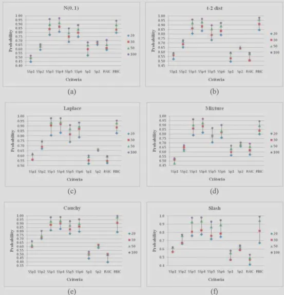
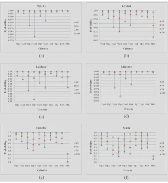
some of the simulation results are summarized in the Tables 1 to 3 and Figures 1 to 4. From Tables 1–3 and Figures 1–4 we observed the following:

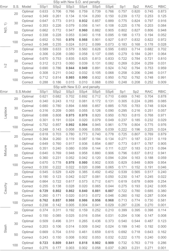
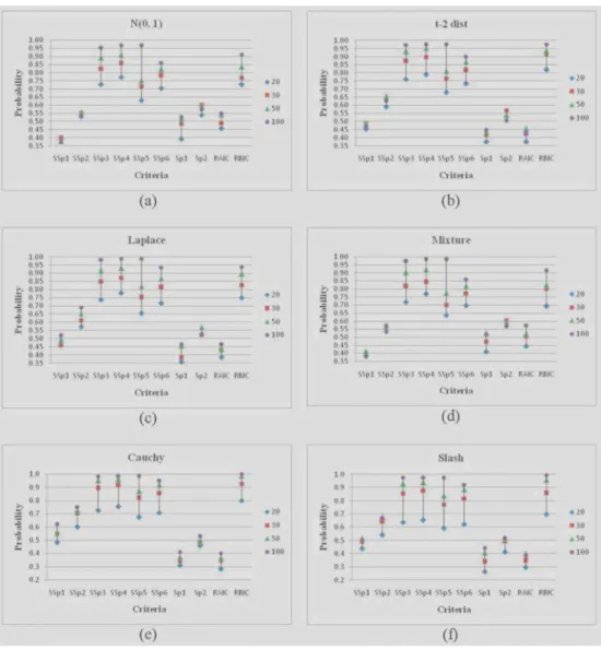
For model IA, predictors X₂ and X₃ are redundant, performance of SSp3 and SSp4 is better than RAIC, Sp1 and Sp2 and it is compatible with RBIC. For model IB, predictor X₃ is redundant, performance of SSp3 and SSp4 is better than RAIC, RBIC, Sp1 and Sp2 (except for Slash distribution). For sample size n=100 and Cauchy and Slash errors, the performance of SSp3, SSp4, SSp5 and SSp6 is better than RAIC, RBIC, Sp1 and Sp2. For Model IC which is full as well as optimal model, perfor-mance of SSp1 is compatible with Sp1, Sp2, RAIC and RBIC for large sample size.

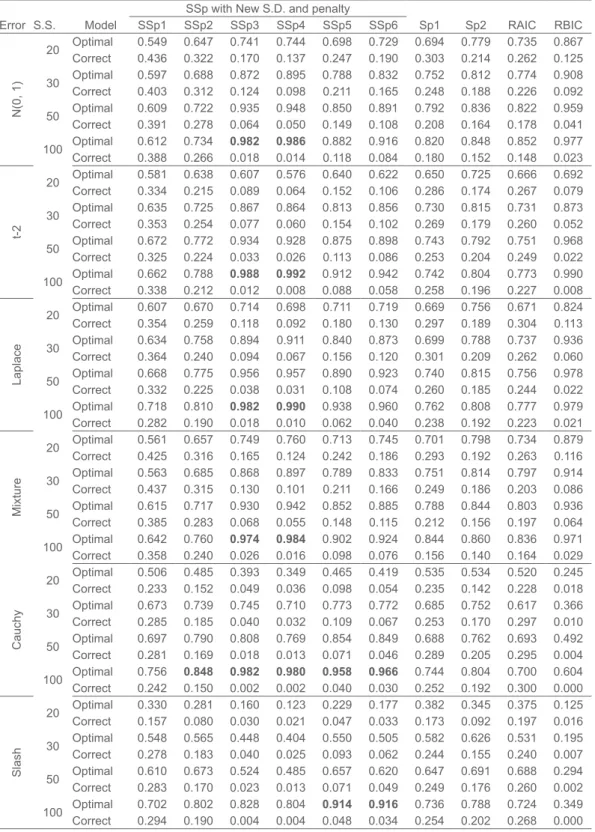
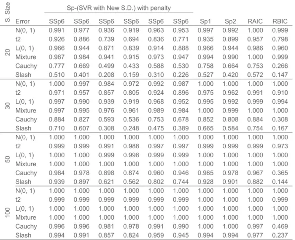
For Model IIA, performance of SSp3, SSp4, SSp5 and SSp6 is better than SSp1, SSp2, RAIC, Sp1 and Sp2. Also it is compatible with RBIC. The performance of SSp2 is better than SSp1, SSp4 is better than SSp3, and SSp6 is better than SSp5 (except for large sample). For Models IIB and IIC, the performance of SSp3, SSp4, SSp5 and SSp6 is better than SSp1, SSp2, RAIC, Sp1 and Sp2, and is compatible with RBIC. Model IID is full model and optimal model. For this model, performance of SSp1 is compatible with Sp1, Sp2, RAIC and RBIC for large sample size. For

Table 1. Probabilities of selecting Optimal and Over fitted (Correct) models for Model I B

Error S.S. Model SSp1 SSp2SSp with New S.D. and penaltySSp3 SSp4 SSp5 SSp6 Sp1 Sp2 RAIC RBIC

N(0, 1) 20 Optimal 0.633 0.706 0.766 0.759 0.739 0.766 0.757 0.820 0.745 0.873 Correct 0.349 0.261 0.134 0.104 0.200 0.150 0.239 0.172 0.253 0.125 30 Optimal_Correct 0.647_0.353 0.773_0.226 0.913_{0.079 0.056}0.932 _0.1410.857 _0.1080.889 _0.2250.775 _0.1760.824 _0.2030.797 0.916_0.084 50 Optimal_Correct 0.662_0.338 0.772_0.228 0.947_{0.053 0.040}0.960 0.882_{0.118 0.095}0.905 _0.1980.802 _0.1730.827 _0.1940.806 0.948_0.052 100 Optimal_{Correct 0.348}0.652 _0.2350.765 0.976 0.988_{0.024 0.012} 0.901_0.099 0.927_0.073 0.817_0.183 0.832_0.168 0.822_0.178 0.972_0.028 t-2 20 Optimal_Correct 0.589_0.306 0.633_0.208 0.579_{0.080 0.058}0.560 _0.1370.628 _0.0950.595 _0.2790.653 _0.1840.714 _0.2610.682 0.702_0.064 30 Optimal 0.670 0.753 0.835 0.825 0.813 0.833 0.722 0.784 0.721 0.810 Correct 0.312 0.213 0.060 0.039 0.131 0.082 0.269 0.204 0.259 0.031 50 Optimal_{Correct 0.308}0.690 0.786_0.211 0.944 0.949_{0.042 0.032} 0.891_0.105 0.924_0.068 0.742_0.258 0.794_0.206 0.753_0.246 0.959_0.017 100 Optimal_{Correct 0.288}0.712 _0.1860.814 0.985 0.990_{0.015 0.010} 0.932_0.068 0.950_0.050 0.752_0.248 0.792_0.208 0.748_0.252 0.991_0.009

Error S.S.Model SSp1 SSp2SSp with New S.D. and penaltySSp3 SSp4 SSp5 SSp6 Sp1 Sp2 RAIC RBIC

Laplace 20 Optimal_Correct 0.621_0.340 0.682_0.243 0.702_{0.112 0.081}0.692 _0.1720.712 _0.1310.710 _0.3050.669 _0.2240.740 _0.2850.704 0.878_0.085 30 Optimal 0.680 0.780 0.894 0.888 0.857 0.885 0.705 0.783 0.748 0.924 Correct 0.316 0.209 0.065 0.055 0.126 0.090 0.295 0.216 0.251 0.057 50 Optimal_{Correct 0.301}0.698 _0.1910.808 0.975 0.978_{0.024 0.020} 0.920_0.079 0.950_0.049 0.763_0.237 0.815_0.185 0.768_0.232 0.971_0.029 100 Optimal_{Correct 0.248}0.752 _0.1430.857 0.992 0.994_{0.008 0.006} 0.945_0.055 0.961_0.039 0.778_0.222 0.804_0.196 0.775_0.225 0.976_0.024 Mixture 20 Optimal_Correct 0.618_0.364 0.703_0.260 0.780_{0.119 0.087}0.773 _0.1940.740 _0.1340.778 _0.2710.725 _0.1870.807 _0.2310.769 0.879_0.119 30 Optimal_Correct 0.649_0.351 0.760_0.240 0.917_{0.080 0.059}0.936 _0.1440.854 0.887_{0.111 0.227}0.773 _0.1830.817 _0.2130.787 0.905_0.094 50 Optimal 0.640 0.769 0.948 0.958 0.880 0.906 0.796 0.837 0.812 0.941 Correct 0.360 0.231 0.052 0.042 0.120 0.094 0.204 0.163 0.188 0.059 100 Optimal_{Correct 0.330}0.670 _0.2220.778 0.978 0.980_{0.022 0.020} 0.902_0.098 0.935_0.065 0.829_0.171 0.848_0.152 0.809_0.191 0.954_0.046 Cauchy 20 Optimal_Correct 0.545_0.190 0.529_0.123 0.429_{0.042 0.027}0.385 _0.0810.492 _0.0500.452 _0.2300.539 _0.1470.565 _0.2450.517 0.240_0.022 30 Optimal_Correct 0.664_0.255 0.722_0.138 0.617_{0.028 0.020}0.573 _0.0650.712 _0.0440.671 _0.2750.619 _0.1930.678 _0.2420.609 0.254_0.005 50 _CorrectOptimal 0.729 0.802 0.862 0.840 0.881 0.887_{0.260 0.171 0.020 0.013 0.072 0.046} 0.722_0.260 0.780_0.192 0.685_0.287 0.380_0.004 100 Optimal 0.762 0.857 0.988 0.986 0.956 0.968 0.713 0.774 0.730 0.581 Correct 0.238 0.142 0.005 0.004 0.041 0.029 0.287 0.226 0.270 0.001 Slash 20 Optimal 0.374 0.311 0.192 0.159 0.252 0.210 0.399 0.395 0.398 0.114 Correct 0.150 0.085 0.025 0.016 0.054 0.031 0.204 0.106 0.147 0.008 30 Optimal 0.509 0.496 0.311 0.265 0.436 0.373 0.540 0.544 0.487 0.123 Correct 0.203 0.106 0.014 0.009 0.042 0.024 0.199 0.140 0.192 0.000 50 Optimal 0.669 0.704 0.510 0.461 0.659 0.615 0.692 0.718 0.643 0.162 Correct 0.243 0.150 0.008 0.002 0.053 0.032 0.222 0.170 0.240 0.000 Optimal 0.723 0.809 0.841 0.818 0.902 0.909 0.732 0.763 0.719 0.286

Table 2. Probabilities of Selecting Optimal and Over fitted (Correct) models for Model II C

Error S.S. Model

SSp with New S.D. and penalty

Sp1 Sp2 RAIC RBIC SSp1 SSp2 SSp3 SSp4 SSp5 SSp6 N(0, 1) 20 Optimal_Correct 0.549_0.436 0.647_0.322 0.741_{0.170 0.137}0.744 _0.2470.698 _0.1900.729 _0.3030.694 _0.2140.779 _0.2620.735 0.867_0.125 30 Optimal_Correct 0.597_0.403 0.688_0.312 0.872_{0.124 0.098}0.895 0.788_{0.211 0.165}0.832 _0.2480.752 _0.1880.812 _0.2260.774 0.908_0.092 50 Optimal_Correct 0.609_0.391 0.722_0.278 0.935_{0.064 0.050}0.948 _0.1490.850 _0.1080.891 _0.2080.792 _0.1640.836 _0.1780.822 0.959_0.041 100 Optimal 0.612 0.734 0.982 0.986 0.882 0.916 0.820 0.848 0.852 0.977 Correct 0.388 0.266 0.018 0.014 0.118 0.084 0.180 0.152 0.148 0.023 t-2 20 Optimal_Correct 0.581_0.334 0.638_0.215 0.607_{0.089 0.064}0.576 _0.1520.640 _0.1060.622 _0.2860.650 _0.1740.725 _0.2670.666 0.692_0.079 30 Optimal_Correct 0.635_0.353 0.725_0.254 0.867_{0.077 0.060}0.864 _0.1540.813 _0.1020.856 _0.2690.730 _0.1790.815 _0.2600.731 0.873_0.052 50 Optimal_Correct 0.672_0.325 0.772_0.224 0.934_{0.033 0.026}0.928 _0.1130.875 _0.0860.898 _0.2530.743 _0.2040.792 _0.2490.751 0.968_0.022 100 Optimal_{Correct 0.338}0.662 _0.2120.788 0.988 0.992_{0.012 0.008} 0.912_0.088 0.942_0.058 0.742_0.258 0.804_0.196 0.773_0.227 0.990_0.008 Laplace 20 Optimal 0.607 0.670 0.714 0.698 0.711 0.719 0.669 0.756 0.671 0.824 Correct 0.354 0.259 0.118 0.092 0.180 0.130 0.297 0.189 0.304 0.113 30 Optimal_Correct 0.634_0.364 0.758_0.240 0.894_{0.094 0.067}0.911 _0.1560.840 _0.1200.873 _0.3010.699 _0.2090.788 _0.2620.737 0.936_0.060 50 Optimal_Correct 0.668_0.332 0.775_0.225 0.956_{0.038 0.031}0.957 _0.1080.890 _0.0740.923 _0.2600.740 _0.1850.815 _0.2440.756 0.978_0.022 100 Optimal_{Correct 0.282}0.718 _0.1900.810 0.982 0.990_{0.018 0.010} 0.938_0.062 0.960_0.040 0.762_0.238 0.808_0.192 0.777_0.223 0.979_0.021 Mixture 20 Optimal_Correct 0.561_0.425 0.657_0.316 0.749_{0.165 0.124}0.760 _0.2420.713 _0.1860.745 _0.2930.701 _0.1920.798 _0.2630.734 0.879_0.116 30 Optimal 0.563 0.685 0.868 0.897 0.789 0.833 0.751 0.814 0.797 0.914 Correct 0.437 0.315 0.130 0.101 0.211 0.166 0.249 0.186 0.203 0.086 50 Optimal_Correct 0.615_0.385 0.717_0.283 0.930_{0.068 0.055}0.942 _0.1480.852 0.885_{0.115 0.212}0.788 _0.1560.844 _0.1970.803 0.936_0.064 100 Optimal_{Correct 0.358}0.642 _0.2400.760 0.974 0.984_{0.026 0.016} 0.902_0.098 0.924_0.076 0.844_0.156 0.860_0.140 0.836_0.164 0.971_0.029 Cauchy 20 Optimal_Correct 0.506_0.233 0.485_0.152 0.393_{0.049 0.036}0.349 _0.0980.465 _0.0540.419 _0.2350.535 _0.1420.534 _0.2280.520 0.245_0.018 30 Optimal_Correct 0.673_0.285 0.739_0.185 0.745_{0.040 0.032}0.710 _0.1090.773 _0.0670.772 _0.2530.685 _0.1700.752 _0.2970.617 0.366_0.010 50 Optimal 0.697 0.790 0.808 0.769 0.854 0.849 0.688 0.762 0.693 0.492 Correct 0.281 0.169 0.018 0.013 0.071 0.046 0.289 0.205 0.295 0.004 100 _CorrectOptimal _0.2420.756 0.848 0.982 0.980 0.958 0.966_{0.150 0.002 0.002 0.040 0.030} 0.744_0.252 0.804_0.192 0.700_0.300 0.604_0.000 Slash 20 Optimal_Correct 0.330_0.157 0.281_0.080 0.160_{0.030 0.021}0.123 _0.0470.229 _0.0330.177 _0.1730.382 _0.0920.345 _0.1970.375 0.125_0.016 30 Optimal_Correct 0.548_0.278 0.565_0.183 0.448_{0.040 0.025}0.404 _0.0930.550 _0.0620.505 _0.2440.582 _0.1550.626 _0.2400.531 0.195_0.007 50 Optimal_Correct 0.610_0.283 0.673_0.170 0.524_{0.023 0.013}0.485 _0.0710.657 _0.0490.620 _0.2490.647 _0.1760.691 _0.2600.688 0.294_0.002 100 Optimal 0.702 0.802 0.828 0.804 0.914 0.916 0.736 0.788 0.724 0.349 Correct 0.294 0.190 0.004 0.004 0.048 0.034 0.254 0.202 0.268 0.000

Table 3. Probabilities of selecting Optimal (and Correct model) for Model II D S. Size Error

Sp-(SVR with New S.D.) with penalty

Sp1 Sp2 RAIC RBIC SSp6 SSp6 SSp6 SSp6 SSp6 SSp6 20 N(0, 1) 0.991 0.977 0.936 0.919 0.963 0.953 0.997 0.992 1.000 0.999 t2 0.926 0.886 0.739 0.694 0.836 0.771 0.935 0.899 0.957 0.798 L(0, 1) 0.966 0.944 0.871 0.839 0.914 0.888 0.966 0.944 0.986 0.960 Mixture 0.987 0.984 0.941 0.915 0.973 0.947 0.994 0.990 1.000 0.999 Cauchy 0.777 0.669 0.499 0.433 0.588 0.530 0.758 0.664 0.753 0.266 Slash 0.510 0.401 0.208 0.159 0.310 0.226 0.527 0.420 0.572 0.147 30 N(0, 1) 1.000 0.997 0.984 0.972 0.992 0.987 1.000 1.000 1.000 1.000 t2 0.971 0.957 0.857 0.805 0.924 0.896 0.975 0.962 0.991 0.910 L(0, 1) 0.997 0.990 0.939 0.919 0.968 0.952 0.995 0.992 0.999 0.994 Mixture 0.997 0.995 0.976 0.961 0.989 0.984 1.000 0.999 1.000 1.000 Cauchy 0.884 0.827 0.593 0.536 0.753 0.678 0.852 0.808 0.884 0.308 Slash 0.710 0.607 0.308 0.248 0.475 0.389 0.665 0.584 0.754 0.167 50 N(0, 1) 1.000 1.000 1.000 1.000 1.000 1.000 1.000 1.000 1.000 1.000 t2 0.999 0.999 0.991 0.988 0.997 0.997 0.999 0.999 0.999 0.973 L(0, 1) 1.000 1.000 0.999 0.998 0.999 0.999 1.000 1.000 1.000 1.000 Mixture 1.000 1.000 1.000 1.000 1.000 1.000 1.000 1.000 1.000 1.000 Cauchy 0.984 0.978 0.898 0.874 0.960 0.946 0.985 0.978 0.967 0.365 Slash 0.939 0.897 0.621 0.562 0.802 0.744 0.928 0.901 0.882 0.144 100 N(0, 1) 1.000 1.000 1.000 1.000 1.000 1.000 1.000 1.000 1.000 1.000 t2 0.999 0.999 0.999 0.999 0.999 0.999 1.000 1.000 1.000 0.999 L(0, 1) 1.000 1.000 1.000 1.000 1.000 1.000 1.000 1.000 1.000 1.000 Mixture 1.000 1.000 1.000 1.000 1.000 1.000 1.000 1.000 1.000 1.000 Cauchy 0.996 0.996 0.981 0.978 0.991 0.990 1.000 1.000 0.997 0.469 Slash 0.994 0.991 0.857 0.824 0.959 0.945 0.994 0.994 0.977 0.237

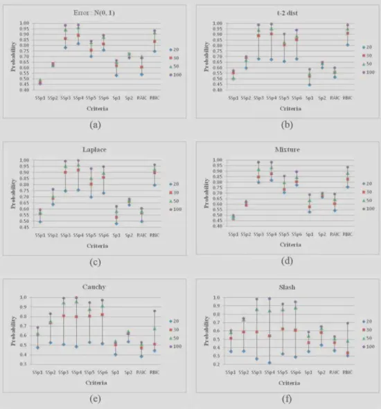
large samples almost all criteria select optimal model with probability 1 except for Cauchy and Slash errors. For small samples (n=20) the performance of RBIC is greater than SSp so, for a small sample size it is suggested to use RBIC.

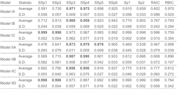
In the simulation, for every model there are six different values of probabilities of selecting optimal model corresponding to six different error distributions. For sample size n=100, obtain the average and standard deviation of these six probabilities for each model. The results are reported in Table 4.

From the summary statistics it is observed that when full model is an optimal model then SSp1 and SSp2 perform better than all other statistics considered in this simulation. When full model is not an optimal model then SSp3 and SSp4 works better than others.

Figure 1. Probabilities of selecting optimal model : Model-I A

Real Data Application

Example 1: To observe the performance of various criteria, consider Brownlee’s

stack loss data(Hand et al., 1994, pp 156) which contains observations from 21 days operation of a plant for the oxidation of ammonia as a stage in the production of nitric acid. The predictor variables are X₁= air flow, X₂= cooling water inlet temperature

(o _{C), X}

3= acid concentration (%) and the response variable Y = stack loss. Stack

As mentioned in Montgomery et al. (2006, p. 396) observation no. 21 is an influential observation because it has a standardized residual of –2.64 from LS fit (Rousseuw & Leroy, 1987, p. 226/227; Rousseuw & van Zomeren, 1990). For a sin-gle outlier, replace observation 21 by 7.5 instead of original value 1.5. As a result, standardized residual corresponding to observation no. 21 becomes 4.01 from LS fit, which indicates that observation no. 21 is a potential outlier. Similarly, for two outliers, replace observation 21 by 7.5 and observation14 by 6 instead of original value 1.2, the corresponding standardized residuals from LS fit are 2.63 and 2.56 respectively, which indicates that observations 21 and 14 are outliers.

For original and outlier data, calculate the SSp statistic with various penalties and

2 2 ˆ ,

σ Sp statistic using SVR (with C = MQD and ε = C ×10-6_{) estimates and M-}

estimator, also Cp statistic using LS. Sp1 refers to the Sp statistic using M estimator and 2

1 ˆ

σ and Sp2 for Sp statistic using M estimator and 2 2 ˆ .

σ Also, for comparison purpose, calculate RAIC and RBIC for the original and outlier data. The results are presented in the Table 5.

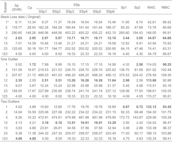
For the original data, all statistics Sp, Cp, SSp with all penalties, Sp1, Sp2, RAIC and RBIC select the subset {X₁, X₂}. For one outlier, statistics Sp, SSp with all

penalties and RAIC select the same subset {X₁, X₂} but Cp, Sp2 and RBIC select wrong subset {X₁}. For two outliers, statistics SSp with all penalties select the same subset {X₁, X₂}, while others select wrong subsets. In particular, Sp and Cp select subset {X₁, X₂, X₃} and Sp1, Sp2, RAIC and RBIC select subset {X₁}.

Example 2: Consider the wine quality datafromMontgomery et al. (2006, Table

B.14, p. 578), which contains 38 observations on response variable wine quality (Y)

based on five predictor variables as clarity (X₁), aroma (X₂), body (X₃), flavor (X₄)

Table 4. Summary Statistics for probability of selecting optimal model for sample size n=100

Model Statistic SSp1 SSp2 SSp3 SSp4 SSp5 SSp6 Sp1 Sp2 RAIC RBIC Model IA Average 0.591 0.730 0.971 0.975 0.898 0.925 0.610 0.658 0.602 0.970 S.D. 0.058 0.057 0.009 0.007 0.033 0.027 0.056 0.033 0.086 0.025 Model IB Average 0.712 0.813 0.960 0.959 0.923 0.942 0.770 0.802 0.767 0.793 S.D. 0.044 0.039 0.059 0.069 0.025 0.022 0.046 0.033 0.042 0.294 Model IC Average 0.999 0.998 0.973 0.967 0.993 0.992 0.999 0.998 0.996 0.759 S.D. 0.002 0.004 0.062 0.077 0.015 0.019 0.002 0.004 0.010 0.354 Model IIA Average 0.476 0.641 0.973 0.979 0.979 0.905 0.469 0.538 0.467 0.956 S.D. 0.093 0.079 0.011 0.009 0.009 0.038 0.045 0.028 0.079 0.039 Model IIB Average 0.569 0.715 0.987 0.990 0.901 0.933 0.612 0.666 0.608 0.896 S.D. 0.082 0.081 0.006 0.007 0.042 0.033 0.059 0.031 0.072 0.107 Model IIC Average 0.682 0.790 0.956 0.956 0.918 0.937 0.775 0.819 0.777 0.812 S.D. 0.053 0.040 0.063 0.075 0.027 0.022 0.046 0.028 0.060 0.272 Model IID Average 0.998 0.998 0.973 0.967 0.992 0.989 0.999 0.999 0.996 0.784 S.D. 0.003 0.004 0.057 0.071 0.016 0.022 0.002 0.002 0.009 0.342

and oakiness (X₅). Test this data for outliers and multicollinearity using Minitab. This data contains only one influential observation, which is observation 20 that has a standardized residual of 2.74. Apply the procedure described in Example 1 for subset selection to this original data. Use all the considered criteria SSp with all penalties, Cp, Sp, Sp1, Sp2, RAIC and RBIC, and select the subset {X₂, X₄, X₅}.

For a single outlier, replace observation 20 by 39.5 instead of original value 7.9, as a result its standardized residual become 5.51, which indicates that observation 20 is a potential outlier. Apply the same procedure for this outlier data. Using the criteria SSp2, SSp3, SSp4, SSp5 and SSp6, select the subset {X₂, X₄, X₅}. The criteria Sp1, Sp2 and RAIC select a different subset {X₁, X₃, X₄, X₅} and RBIC selects the subset {X₄}.

Discussion

The modified Sp criterion was used for subset selection in regression in the presence of outliers and/or error distribution is non normal. Implementation of modified Sp criterion requires a penalty term. The choices for the penalty terms are not limited to those mentioned in this paper. A more suitable penalty can give superior perfor-mance than listed here. The proposed modification makes the criterion free from assumption of the distribution of errors and is even mitigates the effect of outliers. The simulation results confirm these findings.

References

Akaike, H. (1973). Information theory and an extension of the maximum likelihood principle. In B. N. Petrov, & F. Csaki (Eds.), Proceedings of the Second International Symposium of Information Theory (pp. 267-281). Budapest: Akademiai Kiado.

Baierl, A., Futschik, A., Bogdan, M., & Bieecek, P. (2007). Locating multiple interacting quantitative trait loci using robust model selection. Computational Statistics and Data Analysis, 51(12), 6423-6434. doi: 10.1016/j.csda.2007.02.010

Birkes, D., & Dodge, Y. (1993). Alternative Methods of Regression. New York: John Wiley

and Sons, Inc. doi: 10.1002/9781118150238

Boser, B. E., Guyon, I. M., & Vapnik, V. N. (1992). A training algorithm for optimal margin classifiers. COLT ‘92 Proceedings of the fifth annual workshop on Computational learning theory (pp. 144-152). New York: ACM. doi: 10.1145/130385.130401

Table 5. Model selection for Brownlee’s stack loss data.

Subset

Sp

(SVM) Cp _{SSp1 SSp2 SSp3}SSp_{SSp4 SSp5 SSp6} Sp1 Sp2 RAIC RBIC

Stack Loss data ( Original)

1* 6.11 13.34 9.37 11.37 16.54 18.54 18.54 15.46 11.95 8.74 42.91 68.42 2 118.77 28.93 182.28 184.28 189.44 191.44 191.44 188.37 65.20 47.69 73.78 80.69 3 290.65 148.26 446.06 448.06 453.22 455.22 455.22 452.15 265.80 194.43 148.05 95.91 12 2.63 2.95 2.97 5.97 13.71 16.71 16.71 12.10 3.44 3.05 34.07 64.60 13 7.51 14.39 10.46 13.46 21.21 24.21 24.21 19.59 12.82 9.91 43.94 70.93 23 125.65 30.16 191.77 194.77 202.52 205.52 205.52 200.90 64.15 47.46 74.41 83.31 123 4.00 4.00 4.00 8.00 18.33 22.33 22.33 16.18 4.40 4.30 34.79 66.67 One Outlier 1 5.52 1.72 7.99 9.99 15.15 17.15 17.15 14.08 4.32 2.58 114.03 90.25 2 151.59 18.67 219.53 221.53 226.70 228.70 228.70 225.62 136.70 81.69 201.02 102.48 3 337.67 21.72 489.03 491.03 496.20 498.20 498.20 495.12 375.53 224.42 276.59 109.30 12 2.35 2.05 2.51 5.51 13.26 16.26 16.26 11.64 2.98 2.59 113.86 92.88 13 9.07 3.67 12.24 15.24 22.98 25.98 25.98 21.37 5.45 4.06 115.51 93.19 23 158.05 17.87 227.99 230.99 238.74 241.74 241.74 237.12 129.06 77.93 198.61 105.05 123 4.00 4.00 4.00 8.00 18.33 22.33 22.33 16.18 4.09 4.05 115.27 95.81 Two Outliers 1 4.02 4.88 10.60 12.60 17.76 19.76 19.76 16.69 0.87 0.72 132.12 93.45 2 14.04 16.59 225.06 227.06 232.22 234.22 234.22 231.15 82.33 68.48 194.30 101.75 3 8.26 10.22 472.81 474.81 479.98 481.98 481.98 478.90 172.73 143.67 229.06 105.28 12 4.13 4.21 3.16 6.16 13.91 16.91 16.91 12.29 2.50 2.42 134.02 96.47 13 3.83 4.66 23.81 26.81 34.56 37.56 37.56 32.94 3.06 2.88 133.38 96.37 23 9.38 11.38 244.32 247.32 255.07 258.07 258.07 253.45 71.93 60.17 188.15 103.88 123 4.00 4.00 4.00 8.00 18.33 22.33 22.33 16.18 4.75 4.63 135.34 99.41

Bozdogan H., & Haughton D. M. A. (1998). Informal complexity criteria for regres-sion models. Computational Statistics and Data Analysis, 28(1), 51-76. doi: 10.1016/ s0167-9473(98)00025-5

Christmann, A., & Van Messem, A. (2008). Bouligand derivatives and robustness of support vector machines for regression. Journal of Machine Learning Research, 9, 623–644. Christmann, A., Van Messem, A., Steinwart, I. (2009). On consistency and robustness

prop-erties of support vector machines for heavy-tailed distributions. Statistics and Its Inter-face, 2(3), 311–327. doi: 10.4310/sii.2009.v2.n3.a5

Desai, S. S., & Kashid, D. N. (2015). Estimation of regression parameters using svm with new methods for meta parameter. International Journal of Data Mining, Modeling and Management, 7(3), 239-256. doi: 10.1504/ijdmmm.2015.071449

Draper, N. R., & Smith, H. (2003). Applied regression analysis, Third edition. New York:

John Wiley and Sons, Inc.

Gunn, S. R. (1998). Support vector machines for classification and regression (Technical Report). School of Electronics and Computer Science, University of Southampton. Hand, D. J., Daly, F., Lunn, A. D., McConway, K. J., & Ostrowski, E. (1994). A handbook

of small data sets. London: Chapman and Hall. doi: 10.1007/978-1-4899-7266-8

Hocking, R. R. (1976). The analysis and selection of variables in linear regression. Biomet-rics, 32(1), 1-49. doi: 10.2307/2529336

Huber, P. J. (1981). Robust Statistics. New York: John Wiley and Sons, Inc. doi: 10.1002/0471725250

Jaeckel, L. A. (1972). Estimating regression coefficients by minimizing the dispersion of the residuals. Annals of Mathematical Statistics, 43(5), 1449-1458. doi: 10.1214/ aoms/1177692377

Kashid, D. N., & Kulkarni, S. R. (2002). A more general criteria for subset selection in multiple linear regressions. Communication in Statistics Theory and Method, 31(5), 795-811. doi: 10.1081/sta-120003653

Kundu, D., & Murali, G. (1996). Model selection in linear regression. Computational Sta-tistics and Data Analysis, 22(5), 461-469. doi: 10.1016/0167-9473(96)00008-4

Mallow, C. L. (1973). Some comments on Cp. Technometrics, 15(4), 661-675. doi:

10.1080/00401706.1973.10489103

Miller, A. J. (2002). Subset Selection in Regression. Chapman and Hall. doi: 10.1201 /9781420035933

Montgomery, D. C., Peck, E. A., & Vining, G. G. (2006). Introduction to linear regression analysis, Third edition. New York: John Wiley and Sons Inc.

Nalbantov, G. (2003). Short horizon value growth style rotation with support vector machines (Unpublished doctoral thesis). Maastricht University, Netherlands.

Rao, C. R., and Wu, Y. (1989). A strongly consistent procedure for model selection in regres -sion problem. Biometrika, 71, 43-49.

Ronchetti, E. (1985). Robust model selection in regression. Statistics & Probability Let-ters, 3(1), 21-23. doi: 10.1016/0167-7152(85)90006-9

Ronchetti, E., & Staudte, R. G. (1994). A robust version of Mallow’s Cp. Journal of The Amer-ican Statistical Association, 89(426), 550-559. doi: 10.1080/01621459.1994.10476780

Rousseeuw, P. J., & Leroy A. M. (1987). Robust regression and outlier detection. New York:

John Wiley and Sons, Inc. doi: 10.1002/0471725382

Rousseeuw, P. J., & van Zomeren, B. C. (1990). Unmasking multivariate outliers and leverage points. Journal of the American Statistical Association, 85(411), 633-639. doi:

10.1080/01621459.1990.10474920

Schwarz, G. (1978). Estimating the dimension of a model. Annals of Statistics, 6(2), 461-464. doi: 10.1214/aos/1176344136

Shibata, R. (1981). An optimal selection of regression variables. Biometrika, 68(1), 45-54. doi: 10.1093/biomet/68.1.45

Smola, A. J., & Schölkopf, B. (2004). A tutorial on support vector regression. Statistics and Computing, 14(3), 199-222. doi: 10.1023/b:stco.0000035301.49549.88

Thompson, M. L. (1978a). Selection of variables in multiple regression: Part I. A review & evaluation. International Statistical Review, 46(1), 1-19. doi: 10.2307/1402505

Thompson, M. L. (1978b). Selection of variables in multiple regression: Part II. A review & evaluation. International Statistical Review, 46(2), 126-146. doi: 10.2307/1402809

Van Messem, A., & Christmann, A. (2010). A review on consistency and robustness proper-ties of support vector machines for heavy-tailed distributions. Advances in Data Analysis and Classification, 4(2-3), 199–220. doi: 10.1007/s11634-010-0067-2

Vapnik, V., Golowich, S., & Smola, A. (1997). Support vector method for function approx-imation, regression estimation & signal processing. In Mozer, M., Jordan, M., & Petshe, T. (Eds.), Advances in Neural Information Processing Systems 9 (pp. 281-287), Cam-bridge, MA: MIT Press.

Vapnik, V. (2001). The nature of statistical learning theory, Second Edition. New York: