Bayesian Variable Selection via Particle Stochastic Search
Minghui Shia,1, David B. Dunsona,2
aDepartment of Statistical Science, Box 90251, Duke University, Durham, NC, 27708, USA
Abstract
We focus on Bayesian variable selection in regression models. One challenge is to search the huge model space adequately, while identifying high posterior probability regions. In the past decades, the main focus has been on the use of Markov chain Monte Carlo (MCMC) algorithms for these purposes. In this article, we propose a new computational approach based on sequential Monte Carlo (SMC), which we refer to as particle stochastic search (PSS). We illustrate PSS through applications to linear regression and probit models.
Key words: Bayes factor; Marginal inclusion probability; Model averaging; Model uncertainty; Sequential Monte Carlo; Stochastic search variable selection; Subset selection.
1. Introduction
Letyidenote a response variable andxi = (xi1, . . . ,xip)0denote a p×1 vector of candidate
predictors for subjecti,i=1, . . . ,N. Following common notation, letγj=1 denote that the jth
predictor is included in the model withγj =0 otherwise. Then,γ=(γ1, . . . , γp)0is a predictor
inclusion indicator belonging to a model spaceΓ, withΓcontaining 2p elements corresponding
to all possible subsets of thesepcandidate predictors. Conditional onγ, the regression model can be written as
(yi|xγ,i,γ, θγ) ∼ f(xγ,i,γ, θγ) independently (1)
wherexγ,i={1,xi j,j:γj=1}is the predictor vector,θγare the parameters, and pγ =P p j=1γj
is the number of predictors in modelγ.
There is a rich literature on methods for sparse point estimation using methods such as Lasso <Tibshirani, 1996>, the relevance vector machine<Tipping, 2001>and the elastic net<Zou and Hastie, 2005>. Although these sparse point estimation approaches often do a good job in simul-taneously selecting predictors and estimating the coefficients, they do not allow for uncertainty in variable selection. Whenpis moderate to large, there is substantial uncertainty in variable se-lection, and it is important to allow for this uncertainty in conducting predictions and inferences about the important predictors. To obtain more realistic predictive intervals and potentially low-ered mean square predictive error, Bayesian model averaging can be used<Raftery, Madigan,
Email addresses:[email protected](Minghui Shi),[email protected](David B. Dunson)
1Minghui Shi is a graduate student in the Department of Statistical Science, Duke University. 2David B. Dunson is a professor in the Department of Statistical Science, Duke University.
and Hoeting, 1998>. In addition, marginal inclusion probabilities provide a useful measure of the weight of evidence in the data that a particular predictor should be included in the model.
To define a Bayesian approach for variable selection, letπ(γ) denote the prior probability of modelγ. Updating this prior with information in the datay1:N={yi}Ni=1 withX1:N={xi}Ni=1, we
obtain π(γ|y1:N,X1:N) = π(γ)L(y1:N;γ,X1:N) P γ∗∈Γπ(γ∗)L(y1:N;γ∗,X1:N) (2) withL(y1:N;γ,X1:N) = R
L(y1:N;θγ,X1:N)dπ(θγ) the marginal likelihood under model γand L(y1:N;θγ,X1:N) the likelihood ofy1:Nconditionally on the predictorsX1:Nunder (1). Expression
(2) describes the posterior probabilities for each of the candidate models, with these posterior probabilities providing weights to be used in model averaging or a means by which to conduct Bayesian variable selection.
In particular, if the goal is to select a single “best” model, then there are two approaches that are typically used. First, if one chooses a 0-1 loss function in which a loss of 1 is accrued if an incorrect model is selected and it is assumed that the true model is one of those in the listΓ, then the model with lowest Bayes risk corresponds to the highest posterior probability model. Examining expression (2), the posterior probability of modelγis proportional to the prior probability multiplied by the marginal likelihood under that model. Due to the intrinsic Bayesian penalty for model dimension<Jefferys and Berger, 1992>, the marginal likelihood will tend to favor a parsimonious model. However, there are two major problems that arise in selecting the highest posterior probability model when 2pis large. First, the number of models that need to be visited in calculating the denominator in (2) rapidly becomes prohibitively large as p increases, and hence it becomes difficult to accurately estimateπ(γ|y1:N,X1:N). Second,
even if an exact estimate could be obtained, no one model will dominate in large model spaces, and it tends to be the case that many models have similar posterior probabilities to the best model. To address these problems, it has become common to instead select predictors based on thresh-olding of the marginal inclusion probabilities (MIPs), defined as
ζj=P(γj=1|y1:N,X1:N)=
X
γ:γj=1
π(γ|y1:N,X1:N) (3)
for the jth predictor, j=1, . . . ,p. The MIPs provide a weight of evidence that a given predictor should be included adjusting for uncertainty in the other predictors in the model, and hence provide a useful basis for inferences. Barbieri and Berger<2004>showed that the optimal predictive model under squared error loss often corresponds to the median probability model, which includes all predictors having MIPs above 0.5. Because it is often not feasible to visit more than a small fraction of the models inΓin estimating the MIPs, it is important to develop algorithms that efficiently find regions ofΓcontaining high posterior probability models, with such models also tending to have high marginal likelihoods unless the prior is overly informative. George and McCulloch<1993>proposed a stochastic search variable selection (SSVS) algo-rithm for normal linear regression using Gibbs sampling to searchΓfor high posterior probability models. Their approach relies on a mixture of a low and high variance normal prior centered at zero for each of the regression coefficients, with the low variance component corresponding to a predictor being effectively excluded due to the coefficient being close to zero. However, in many applications, this approach is subject to very slow mixing of the Gibbs sampler and hence poor
computational efficiency<George and McCulloch, 1997>. As reviewed in George and McCul-loch<1997>, Geweke<1996>, Carlin and Chib<1995>and Green<1995>propose alternative methods to improve the performance of SSVS. As noted in Liu et al. <1994>, an effective strategy for improving efficiency of MCMC algorithms is marginalization. The most efficient of the available SSVS algorithms (to our knowledge) relies on marginalizing out the regression coefficients in updating the variable inclusion indicators<George and McCulloch, 1997>. In particular, this algorithm iteratively samples the variable inclusion indicator for the jth predic-tor,γj, from its Bernoulli full conditional posterior distribution given the other predictors in the
model,γ(−j)={γl:l, j,l=1, . . . ,p}, for j=1, . . . ,p.
In this article, we propose a sequential Monte Carlo (SMC) approach for obtaining a sampling-based approximation to the posterior distribution ofγ, providing an alternative to SSVS and other MCMC-based methods. Although SMC is commonly used for dynamic models, the application to static models was initially proposed by Chopin<2002>, with Del Moralet al.<2006> provid-ing a general methodology. However, there has been limited work on the use of SMC for model selection. Chopin<2007>used SMC for model choice in hidden Markov models. Toniet al.
<2009>proposed an approximate Bayesian computation method for model selection in dynam-ical systems using SMC. Zhanget al. <2007>proposed an SMC-type sequential optimization approach for variable selection, though their approach does not accommodate uncertainty in the selection process.
Our proposed particle stochastic search (PSS) algorithm relies on introducing a sequence of particle approximations to the partial posterior distributions{π(γ|y1:n,X1:n)}nN=1, with the
parti-cles sequentially updated through rejuvenating and reweighing operations as subjects are added to the data set. By adding data sequentially, we initially allow faster exploration of the model space, as the partial posteriors will be effectively annealed relative to the eventual target. In addition, the algorithm can take advantage of distributed computing on a cluster for more rapid computation. In the sequel, we provide details on the PSS approach and compare it to MCMC algorithms in linear and probit regression.
2. Particle Stochastic Search
Due to the dimensionality problem mentioned in Section 1, we focus primarily on obtaining accurate estimates of the MIPs, though the proposed algorithm can also be used to identify high posterior probability models, as we illustrate in Section 3.
2.1. Sequential Monte Carlo for Variable Selection
Sequential Monte Carlo (SMC) relies on a discrete approximation to the posterior distribution
π(γ|y1:n,X1:n)≈g(γ;{γnm,wnm}mM=1)= M X m=1 wnmδγnm(γ), (4) where{γn
m}Mm=1is a collection of particles,δγdenotes a degenerate distribution with all its mass
atγ, andwn
mis the probability on particleγnm.
Based on the theory of importance sampling <e.g Liu, 2001, Ch.2>, given a particle ap-proximationg(γ;{γn−1
m ,wn−1m }mM=1) to the partial posterior distribution π(γ | y1:n−1,X1:n−1), one
can obtain a particle approximationg(γ;{γn
m,wnm}mM=1) to the partial posterior distributionπ(γ|
y1:n,X1:n) by propagating the particlesγnm=γn−1m and using modified weights wnm= π(γn m|y1:n,X1:n) π(γn−1 m |y1:n−1,X1:n−1) wn−1m , m=1, . . . ,M. (5)
One can start by drawingγ0m∼π(γ),m=1, . . . ,M, choosing equal weights{w0m=1/M}mM=1to
obtain the initial approximation, and then apply (5) recursively to obtain a particle approximation (4) for the posterior distributionπ(γ | y1:N,x1:N). However, this sequential weight-updating
step has the problem that after several iterations, fewer and fewer particles maintain significant weights. To address this degeneracy problem, a common strategy is to remove particles with very low weights by weighted resampling from{γn−1
m }mM=1. Unfortunately, resampling does not
introduce new particles, so this approach leads to few particles having very high weight. LetK(γ?|γ) denote a transition kernel with invariant probability distributionπ(γ|y1:n,X1:n),
π(γ?|y
1:n,X1:n)=
Z
K(γ?|γ)π(γ|y1:n,X1:n)dγ. (6)
Given an initial particle approximationg(γ;{γm,wm}Mm=1), one can use the modified
approxima-tionPM
m=1wmK(γ?m | γm). To draw samples from this approximated distribution, one can first
draw a set of indicators{Im}mM=1indicating whichγmshould be used for the generation ofγ?m, and
then sampleγ?mfromK(γ?m |γIm). The first stage is effectively resampling and the second step allows the generation of fresh particles<Pitt and Shephard, 1999>,<Carvalhoet al.2010>.
We consider the following choices of the transition kernelK(γ?|γ): 1. Metropolis Hasting kernel:
(a) Generate a candidateγ?from probability distributionq(γ?;γ). (b) Accept the candidateγ?with probability
α(γ,γ?)=min(1,q(γ;γ?) q(γ?;γ) L(y1:n;γ?,X1:n)π(γ?) L(y1:n;γ,X1:n)π(γ) ) . (7)
2. Gibbs sampling transition kernel: Letγ(j) =(γ1, . . . , γj−1, γj+1, . . . , γp), andτ=(τ1, . . . , τp)
denote some permutation of{1,2, . . . ,p}. Then for j=τ1,τ2,. . .,τp:
(γj|γ(j))∼Bernoulli( ˆpj) (8) with ˆ pj = π(γ(j), γj=1|y1:n,X1:n) π(γ(j), γj=0|y1:n,X1:n)+π(γ(j), γj=1|y1:n,X1:n) .
In order to introduce more fresh particles which have less dependence with the previous par-ticles, we can use strategies commonly used for improving the convergence of MCMC. For example, one can use a blocked Gibbs sampling transition kernel. In the following algorithm, the Metropolis Hastings kernel is applied within a particle iterativelyptimes.
In choosing between transition kernels, a useful measure of the efficiency is the effective sam-ple size (ESS), defined as
ESS(N)= N
1+var(w), (9)
with var(w) the variance of the importance weights with respect to the proposal distribution. The ESS(N) provides an estimate of the number of independent samples from the target probability measure, which would provide the same estimation precision as the particle approximation. It is common to only resample when ESS(N) becomes low.
We propose two alternative PSS algorithms below.
Algorithm 1. (i) Initialization: Start with sampling the particles{γ0
m}mM=1 from the prior dis-tributionπ(γ).
(ii) For n=1,2, . . . ,N, add the nthobservation(yn,xn)and cycle through a) Reweighting: update the weights of the particles:
wnm∝L(yn;γmn,xn)·wn−1m (10) and setγn
m=γn−1m for m=1, . . . ,M.
b) Calculate the ESS(M) (9) based on the updated weights. Once ESS(M)<M/2: b1) (Resample) Resample{γnm}Mm=1with replacement using weights{wnm}Mm=1using an
efficient sampling strategy. Reset the weights{wnm}Mm=1to{wnm=1/M}mM=1. b2) (Rejuvenation) For any m, replace γnm with a sample from Kn(γ,γnm) where
Kn(· | γ) defines a transition kernel with invariant probability distribution
π(γ|y1:n,X1:n).
Del Moral et al. <2006>proposed alternatives to sequential adding of observations. For simplicity and to facilitate extensions, we do not consider such approaches here.
2.2. Generalization to Latent Variable Models
For the normal linear regression model, the marginal likelihood is available in closed form whenπ(θγ) is chosen as a multivariate normal-gamma prior. However, for generalized linear models, the marginal likelihood is typically analytically intractable. Albert and Chib<1993> and Holmes and Held<2006>demonstrated auxiliary variable approaches for binary regression models. In this section, we describe the modification of the auxiliary variable approach to our PSS algorithm.
To begin, consider a probit regression model
yi ∼ Bernoulli(Φ(ηi)), ηi=xiβ, β∼π(β), (11)
withΦ(·) the cumulative distribution function of a standard normal random variable. A well known augmented formulation for Model (11) is
yi = ( 1 zi>0 0 otherwise , zi=x 0 iβ+i, i∼N(0,1), β∼π(β). (12)
The advantage of (12) is that, for Gaussianπ(β), we can obtain the marginal likelihood condi-tionally on the latent variableszbut marginalizing outβ. Thus, we can extend our PSS algorithm to probit regression models by including the model indexγand the latent variableszwithin the particles.
Theorem 1. (Liu<2001>) Letπ0(x,y)andπ1(x,y)be two probability densities, where the sup-port ofπ0is a subset of the support ofπ1. Then,
varπ1 (π 0(x,y) π1(x,y) ) ≥varπ0 (π 0(x) π1(x) ) , (13) whereπ1(x)= R π1(x,y)dy andπ0(x)= R
π0(x,y)dy are marginal densities.
Based on Theorem 1, we should obtain better performance of the PSS method by avoid putting in the regression parameters specific to each model within the particles and instead marginalizing out these parameters. Marginalization is a common technique for reducing autocorrelation in MCMC algorithms; for example, refer to Holmes and Held<2006>in the setting of SSVS using data augmentation in binary response models.
Let Kn(z?1:n,γ? | z1:n,γ) denote a transition kernel with invariant distribution π(z1:n,γ |
y1:n,X1:n) which can be factorized as Kn(z?1:n,γ?|z1:n,γ)=K
γ
n(γ?,|z?1:n,γ)K z
n(z?1:n|z1:n,γ). (14)
We consider the following choice ofKn(γ?,z?1:n |z1:n,γ)
1. Gibbs sampling kernel:
Knz(z?1:n|z1:n,γ)=p(z?1 |z2:n,γ,y1:n,X1:n) n
Y
i=2
p(z?i |z?1:(i−1),z(i+1):n,γ,y1:n,X1:n). (15)
For probit regression models with a Gaussian prior, we can directly sample from p(z?i | z?1:(i−1),z(i+1):n,γ,y1:n,X1:n) which is a truncated normal distribution.
2. Gibbs sampling or Metropolis Hasting kernels forKnγ(γ?|z?1:n,γ) as in Section 2.1.
Algorithm 2. (i) Initialization: Start with sampling the particles{γ0m}M
m=1 from the prior dis-tributionπ(γ).
(ii) For n=1, . . . ,N, add the observation(yn,xn)and cycle through: a). Reweighting: update the weights of the particles:
wnm∝L(yn;zn−11:n−1,m,γn−1m ,xn)·wn−1m (16) and set(zn 1:n−1,m,γ n m)=(zn−11:n−1,m,γ n−1 m )for m=1, . . . ,M.
b). Propagating: Sample the next latent variable znfor each particle m:
(znn,m|zn1:n−1,m,γnm,yn,xn)∼p(zn|zn1:n−1,m,γ n
m,yn,xn) (17) with the particle system updated to{zn
1:n,m,γ n
m,wnm}mM=1.
c). Calculate the ESS(M) (9) based on the updated weights. If ESS(M)<M/2: c1) (Resample) Resample{zn1:n−1,m,γnm,wnm}Mm=1with replacement using weights{w
n m} based on an efficient sampling strategy. Reset the weights {wn
m}mM=1 to {w n m =
1/M}mM=1.
c2) (Rejuvenation) For any m, replace(zn1:n,m,γnm) with a sample from a transition kernel with the invariant distributionπ(z1:n,γ|y1:n,X1:n).
Compared with MCMC, PSS has the advantage of avoiding mixing problems, such as a ten-dency to remain for long intervals within a local region of the model spaceΓ. However, the tradeoffin SMC algorithms such as PSS is the risk of degeneracy and the potential need to use enormous numbers of particles to obtain an accurate approximation. It is straightforward to extend PSS beyond linear regression and probit models to other models in which marginal like-lihoods are available analytically after augmentation. For example, the nonparametric mixture regression models of Chung and Dunson<2009>fall in this class. PSS can be implemented either in serial or in parallel, though a primary advantage of PSS is the ability to accommodate high-dimensional cases through the use of parallel computing.
2.3. Prior Specification and Extensions
The PSS algorithms described above assume that the marginal likelihoodL(y1:N;γ,X1:N) can
be obtained in closed form, which places some constraints on the priors that can be considered. For example, in normal linear regression, we have assumed that a multivariate normal-gamma joint prior is placed on the regression coefficients and residual precision. This is a standard choice in the literature. SSVS algorithms that rely on marginalizing out the model parameters also require a closed form marginal likelihood, so have similar restrictions on the prior. For both PSS and SSVS, the class of priors and models that can be considered can be expanded by using approximations to the marginal likelihood, such as Laplace.
There are some disadvantages of the multivariate normal-gamma prior, such as lightness of the tails leading to lack of robustness. A number of alternative priors have been proposed, which place hyper-priors on one or more parameters in the multivariate normal-gamma prior. One example is the mixture of g-priors considered in Lianget al. <2008>. In MCMC-based SSVS
algorithms, it is straightforward to include hyper-priors on parameters that are common to the dif-ferent models, and then update these parameters in separate steps from the model index updating steps. In PSS, we can similarly allow richer classes of priors by including the hyper-parameters ψcommon to the different models directly in the particles along with the model indexγ. The algorithm would remain essentially the same as described above, but in the rejuvenation step we would need to apply an invariant transition kernel for the joint posterior of (γ, ψ). For example, we could use a Gibbs transition kernel.
2.4. Bayesian Inference from the Particles
As described in Section 1, there are a variety of approaches available for selecting predictors based on posterior model probabilities, with our emphasis here being on the median probability model that selects those predictors having marginal inclusion probabilities (MIPs) greater than 0.5. However, in many applications it is not necessary to formally select predictors and may be more useful to present a ranked list of the predictors having the highest MIPs along with their MIPs. As the MIPs provide a weight of evidence that a variable should be included as a predictor, such a summary provides more information than simply a list of selected predictors.
After obtaining a particle approximationg(γ;{γN
m,wNm=1}Mm=1) to the complete posterior
dis-tributionπ(γ|y1:N,X1:N) over the model space using PSS, the MIP for the jth predictor can be
estimated as ˆ ζj= 1 M M X m=1 1(γN m,j=1). (18)
After selecting a model based on thresholding of the estimated MIPs, the posterior distribution of the coefficients and residual variance in the selected model can be obtained easily.
3. Examples
3.1. Normal Linear model
We illustrate PSS and compare results to SSVS using simulated examples with the first example taken from George and McCulloch <1997>. To calculate the marginal likelihood
L(y1:N;γ,X1:N) in both methods, we use a simple multivariate normal-gamma prior
distribu-tion forθγ, which includes both the regression coefficientsβγand the residual precisionσ−2in
the linear regression case,
(βγ|σ2,γ)∼N(0, σ2Iγ), (σ2|γ)∼IG(pγ/2,pγλγ/2),
withλγ=s2
LS equal to the classical least square estimate ofσ
2 based on the full model as an
empirical Bayes approach to set the scale<George and McCulloch, 1997>. In addition, we assumed that the elements ofγare iid Bernoulli(0.5) in order to assign equal prior probability to inclusion or exclusion of each predictor.
Algorithms that efficiently discover models with high log-marginal likelihoods will also tend to find models with high posterior probabilities, because the posterior probability is proportional to the prior probability times the marginal likelihood. Hence, we record the log marginal likelihoods of the models visited by PSS and SSVS as one measure of performance, while also estimating MIPs for each of the predictors and the median probability model. Ideally, the MIPs would be close to one for predictors that should be included and close to zero for predictors that should be excluded. However, when important predictors are highly correlated, the MIPs for these predictors will tend to be substantially less than one and may even be less than 0.5. Bayesian variable selection automatically attempts to find a parsimonious model that has good predictive performance, and from this perspective it is often optimal to select one of a correlated set of predictors. The outcomes from all the simulations below are standardized to have mean 0 and unit variance. All of the algorithms are coded in C++, with the PSS algorithms implemented using parallel computation.
Example 1.
GenerateZ1, Z2, . . ., Z15, Z from N100(0,I), and set the covariate Xi to satisfy Xi=Zi+2Z for i=1,3,5,8,9,10,12,13,14,15 with X2=X1+0.15Z1, X4=X3+0.15Z4, X6=X5+0.15Z6, X7=X8+X9
-X10+0.15Z7andX11=X14+X15-X12-X13+0.15Z11. The regression coefficients areβ=(1.5, 0, 1.5, 0, 1.5, 0, 1.5, 1.5, 0, 0, 1.5, 1.5, 1.5, 0, 0)0
. The final observation variables are drawn from
yi ∼N(x0iβ, σ2) withσ2=2.5. Under this construction, there is a strong multicollinearity among
the predictors and the correlations betweenXiandXi+1are as high as 0.998.
We start with this simple example in order to test the performance of PSS in a case in which the true posterior model probabilities and marginal inclusion probabilities (MIPs) can be calculated precisely. As there are 215 = 32,768 models in Γ in this case, it is feasible to calculate the marginal likelihood for every model in the list. For a short run, we set the initial number of particles for PSS to beM=1000. However, our hope is that we can still obtain reasonably accurate estimates of the MIPs and identify many of the top posterior probability models based on a modest number of particles. SSVS also typically relies on many fewer samples than there are models inΓ. Matching implementation time approximately, we ran SSVS for 5000 iterations.
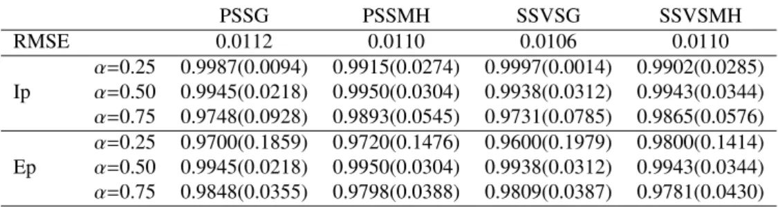
We obtained 50 simulation replicates in order to judge performance across many data sets. For each simulation, both PSS and SSVS found the true highest posterior probability model. Since the true MIPs can be obtained in this case, we can calculate root mean square errors (RMSE) of the estimated MIPs and other summaries of performance. LetbγE(α)={1(ζj > α),j=1, . . . ,p}
denote the model selected by including predictors having exact MIPs larger than a threshold ofα. To assess the relative performance of PSS and SSVS at efficiently approximating exact Bayesian variable selection, we use the following two summaries
Ip(α)= Pp j=11(ζj> α)1( ˆζj> α) Pp j=11(ζj> α) , Ep(α)= Pp j=11(ζj< α)1( ˆζj< α) Pp j=11(ζj< α) 8
withζjand ˆζjthe true and estimated MIPs for predictor j, respectively. Here, Ip(α) denotes the
proportion of predictors in modelbγE(α) that are appropriately included in the model selected using the estimated MIPs, while Ep(α) denotes the proportion of predictors not in modelbγE(α) that are appropriately excluded. Table 1 shows summaries of the RMSE of the estimated MIPs, the means of the Ip and Ep with the standard deviations in the parentheses for both PSS and SSVS. Both PSS and SSVS have excellent performance in terms of accurately approximating Bayesian variable selection based on thresholding of the exact MIPs.
PSSG PSSMH SSVSG SSVSMH RMSE 0.0112 0.0110 0.0106 0.0110 Ip α=0.25 0.9987(0.0094) 0.9915(0.0274) 0.9997(0.0014) 0.9902(0.0285) α=0.50 0.9945(0.0218) 0.9950(0.0304) 0.9938(0.0312) 0.9943(0.0344) α=0.75 0.9748(0.0928) 0.9893(0.0545) 0.9731(0.0785) 0.9865(0.0576) Ep α=0.25 0.9700(0.1859) 0.9720(0.1476) 0.9600(0.1979) 0.9800(0.1414) α=0.50 0.9945(0.0218) 0.9950(0.0304) 0.9938(0.0312) 0.9943(0.0344) α=0.75 0.9848(0.0355) 0.9798(0.0388) 0.9809(0.0387) 0.9781(0.0430)
Table 1: RMSE of the estimated MIPs, Inclusion percentage and Exclusion percentage based on 50 simulation replicates: PSS with Gibbs kernel (PSSG) and PSS with MH kernel (PSSMH), SSVS with Gibbs (SSVSG) and SSVS with MH kernel (SSVSMH)
By adding 85 predictors X16:100 with zero coefficients, we extended p from 15 to 100 and reapplied PSS and SSVS. In this case the number of models inΓis too large to calculate the marginal likelihood for all models, so the highest posterior probability model and MIPs cannot be calculated exactly. Hence, we instead compare the relative performance of PSS and SSVS in identifying high log-marginal likelihood models, in estimating MIPs that are high for predictors that should be in the model and in estimating a median probability model that is close to the true model. Table 2 gives the median, 75th percentile, 95th percentile and maximum for the log-marginal likelihoods found in those methods. In this high dimensional case, PSS with 10,000 particles finds slightly higher posterior probability regions than 20,000 SSVS iterations. Table 3 shows the indexes of the predictors in the estimated models based on different thresholdings. The model selected is sensitive to the choice of the thresholdingα, withα=0.5 often an optimal choice in terms of predictive performance<Barbieri and Berger, 2004>.
Median 75% 95% Maximum
PSSG -281.4936 -280.8975 -280.5607 -280.5072
PSSMH -281.4626 -280.8909 -280.5721 -280.5072
SSVSG -281.5759 -280.9630 -280.6783 -280.6013
SSVSMH -281.5197 -280.9188 -280.6127 -280.5607
Table 2: Summaries of the log-marginal likelihoods for the top models in the linear regression case: PSS with Gibbs kernel (PSSG), PSS with MH kernel (PSSMH), SSVS with Gibbs (SSVSG) and SSVS with MH kernel (SSVSMH).
3.2. Probit Regression Model
We also apply PSS to the following probit regression model with details listed in the Appendix. The prior distribution we used forβγ|γisN(bγ,vγ) withbγ=0 andvγ=Ipγ×pγin examples.
α=0.45 PSSG 2,3,5,6,7,9,14,15 SSVSG 1,2,3,5,7,9,12,13,14,15 PSSMH 2,3,5,6,7,9,14,15 SSVSMH 2,3,5,7,9,13,14,15 α=0.50 PSSG 2,3,5,7,9,14,15 SSVSG 2,3,5,7,9,13,14,15 PSSMH 2,3,5,7,9,14,15 SSVSMH 2,3,5,7,9,14,15 α=0.55 PSSG 3,5,7,9,14,15 SSVSG 3,7,14,15 PSSMH 3,7,9,14,15 SSVSMH 3,7,9,14,15
Table 3: The models selected based on different thresholds on the estimated marginal inclusion probabilities for the linear regression case: PSS with Gibbs kernel (PSSG), PSS with MH kernel (PSSMH), SSVS with Gibbs (SSVSG) and SSVS with MH kernel (SSVSMH).
Example 2:
Choose the covariate matrixX(p)=(1,X) withXthe same as the covariate matrix in the normal linear regression example with 100 predictors. The response variables are drawn from model (11) withηi=x(p)0
iβ(p),zi∼N(ηi,1),yi=1(zi≥0) andβ(p)=(1.5, β) withβalso being taken from p=100 normal linear regression example.
As the marginal likelihood for the probit model is not available analytically, we instead use the complete data marginal likelihood here, which is available for the simulation as we have generatedz. In this example, we compare our PSS algorithm with MCMC. As is illustrated in Table 4, PSS with 10,000 particles found slightly higher posterior regions than 20,000 MCMC iterations. The models selected based on different thresholdsαon the MIPs are listed in Table 5. If the model selected is (1, 2, 3), it corresponds toηi=β0+β1X1+β2X2+β3X3in (11).
Median 75% 95% Maximum
PSSG -129.8118 -121.9266 -111.6871 -105.0315
PSSMH -129.7112 -122.3866 -112.4855 -105.0191
MCMCG -131.5902 -124.8271 -115.2204 -105.0118
MCMCMH -131.4937 -125.0411 -115.8446 -105.0548
Table 4: Summaries of the log complete data marginal likelihood for the top models selected in the probit case: PSS with Gibbs kernel (PSSG), PSS with MH kernel (PSSMH), MCMC with Gibbs (MCMCG) and MCMC with MH kernel (MCMCMH). α=0.45 PSSG 1,3,4,7,9,14,15 MCMCG 1,2,3,4,7,9,10,14,15 PSSMH 1,3,4,7,9,10,14,15 MCMCMH 1,2,3,4,5,7,9,10,14,15 α=0.50 PSSG 3,4,7,9,14,15 MCMCG 2,3,4,7,9,14,15 PSSMH 3,4,7,9,14,15 MCMCMH 1,3,4,7,9,14,15 α=0.55 PSSG 3,4,9,15 MCMCG 3,4,9,14,15 PSSMH 3,4,9,15 MCMCMH 3,4,9,15
Table 5: The models selected based on different thresholdsαon the MIPs in the probit case: PSS with Gibbs kernel (PSSG), PSS with MH kernel (PSSMH), MCMC with Gibbs (MCMCG) and MCMC with MH kernel (MCMCMH).
4. Conclusion
This article has proposed an SMC algorithm for Bayesian variable selection. Our goal in using SMC was to obtain an alternative to MCMC-based SSVS, which may have advantages in certain cases. First, the proposed PSS algorithm has an automatic annealing feature that results from the sequential addition of subjects. This annealing leads to more rapid exploration of the model space initially and then a more concentrated search as subjects are added. Although annealing is also commonly used within MCMC algorithms to limit problems with stickiness when the pos-terior is multimodal, the performance of such algorithms tends to be quite sensitive to difficult to choose tuning parameters, such as temperature ladders. PSS incorporates an implicit temperature sequence through making the target more concentrated as subjects are added, so avoids the need to choose tuning parameters.
A second beneficial feature of PSS is that the approach can take advantage of parallel com-puting environments to simultaneously explore many regions of the model space starting with widely-dispersed particles sampled from the prior. This tends to limit the chance of getting stuck for long intervals in a local region of the model space, and makes it more likely to discover promising regions. Unlike simply implementing SSVS in parallel, PSS automatically commu-nicates across the particles and will discard particles in unpromising low probability regions. Our simulation in thep =100 case provided some initial evidence that PSS has better perfor-mance in finding the top models in large predictor spaces, though more extensive simulations and theoretical studies are needed.
This article is meant as an initial description of a promising new class of algorithms for a very challenging and important problem. Certainly, the challenges of attempting posterior computa-tion in a model space with 2p elements when pis large should not be underestimated. PSS is by no means a perfect alternative to SSVS in that accurate approximation of the posterior of the model indexγwhen pis large would seem to necessitate using an enormous number of parti-cles, which may not be computationally feasible. However, MCMC faces a similar problem in requiring an infeasible number of samples. Hence, it is important to keep in mind that these al-gorithms are designed to search for good models and not to accurately approximate the posterior for largep. Our hope is that the current PSS algorithm will provide a competitive alternative to SSVS that does better in certain applications, while stimulating additional work in this area. In particular, we suspect that more efficient transition kernels can potentially be chosen to improve performance of PSS.
5. Appendix
PSS implementation details for the probit model under the priorβ∼N(b,v). Define
Bγ,n =Vγ,n(v−1γbγ+X
0
1:n,γz1:n), Vγ,n=(v−1+X
0
1:n,γX1:n,γ)−1,
1. Reweighting: After marginalizing out the latent variable for the new observations, the weight (16) satisfies wnm ∝ [1(yn=1){1−Φ(0|µˆn,σˆ2)}+1(yn=0)Φ(0|µˆn,σˆ2)]wn−1m with ˆ µn m = x 0 γn−1 m ,n Vγn−1 m ,n(v −1 γn−1 m bγn−1 m +X 0 1:n,γn−1 m zn−11:n,m), ( ˆσ2)nm = x0γn−1 m ,n Vγn−1 m xγn −1 m ,n+1. 11
2. Propagating: Sample the latent variableznfor the observationynfrom a truncated normal
distribution, (17) satisfies :
(znn,m|zn1:n−1,m,γ,y1:n,X1:n)NAn(zn; ˆµ,σˆ
2),
withAn =(−∞,0] foryn=0 and An =(0,+∞) for yn=1, where NA(µ, σ2) is the N(µ, σ2) distribution truncated toA.
3. Rejuvenating:
(a) To sample from (15), cycle thoughi=1,. . .,n: (zni,m|zn(i),m,γnm,y1:n,X1:n,)∝ ( N(0,+∞)(mi,vi), yi=1 N(−∞,0](mi,vi), yi=0 , with mi=xi,γn mBγnm,n−wi(zi−xiBγmn,n), vi=1+wi, wi=hi/(1−hi) and hi is the ith diagonal element of H = X1:n,γn
mVγnm,nX 0 1:n,γn m , z(i) = (z1, . . . ,zi−1,zi+1, . . . ,zN)
(b) To sampleKnγ(γ?,| z?1:n,γ), we can use the Gibbs sampling kernel or the Metropolis
Hasting kernel mentioned in Section 2.1. Acknowledgements
This research was supported by Grant Number 1R01ES017436-01 from the National Institute of Environmental Health Sciences of the U.S. National Institutes of Health.
References
Albert, J. H., Chib, S., 1993. Bayesian analysis of binary and polychotomous response data. Journal of the American Statistical Association 88, 669–679.
Barbieri, M. M., Berger, J. O., 2004. Optimal predictive model selection. The Annals of Statistics 32, 870–897. Carlin, B. P., Chib, S., 1995. Bayesian model choice via Markov chain Monte Carlo methods. Journal of the Royal
Statistical Society: Series B (Statistical Methodology) 57, 473–484.
Carvalho, C., Johannes, M., Lopes, H., Polson, N., 2010. Particle learning and smoothing. Statistical Science 25, 88–106. Chopin, N., 2002. A sequential particle filter method for static models. Biometrika 83, 539–552.
Chopin, N., 2007. Inference and model choice for sequentially ordered hidden markov models. Journal of the Royal Statistical Society: Series B (Statistical Methodology) 69, 269–284.
Chung, Y., Dunson, D. B., 2009. Nonparametric Bayesian conditional distribution modeling with variable selection. Journal of American Statistical Association 104, 1646–1660.
George, E. I., McCulloch, R. E., 1993. Variable selection via Gibbs sampling. Journal of the American Statistical Asso-ciation 88, 881–889.
George, E. I., McCulloch, R. E., 1997. Approaches for Bayesian variable selection. Statistica Sinica 7, 339–374. Geweke, J., 1996. Variable selection and model comparison in regression. In: Bernardo, J. M., Berger, J. O., Dawid, A. P.,
Smith, A. F. M. (Eds.), Bayesian Statistics 5 – Proceedings of the Fifth Valencia International Meeting. Clarendon Press [Oxford University Press], pp. 609–620.
Green, P. J., 1995. Reversible jump markov chain Monte Carlo computation and Bayesian model determination. Biometrika 82, 711–732.
Holmes, C. C., Held, L., 2006. Bayesian auxiliary variable models for binary and multinomial regression. Bayesian Analysis, 145–168.
Jefferys, W. H., Berger, J. O., 1992. Ockham’s razor and Bayesian analysis. American Scientist 80, 64–72. Liu, J. S., 2001. Monte Carlo Strategies in Scientific Computing. Springer Series in Statistics.
Pitt, M. K., Shephard, N., 1999. Filtering via simulation: Auxiliary particle filters. Journal of the American Statistical Association 94, 590–599.
Raftery, A. E., Madigan, D., Hoeting, J. A., 1998. Bayesian model averaging for linear regression models. Journal of the American Statistical Association 92, 179–191.
Tibshirani, R., 1996. Regression shrinkage and selection via the lasso. Journal of the Royal Statistical Society: Series B (Statistical Methodology) 58, 267–288.
Tipping, M. E., 2001. Sparse Bayesian learning and the relevance vector machine. Journal of Machine Learning Research 1, 211–244.
Zou, H., Hastie, T., 2005. Regularization and variable selection via the elastic net. Journal of the Royal Statistical Society: Series B (Statistical Methodology) 67, 301–320.