D-Rules : Learning & Planning
Silvana Roncagliolo Escuela de Ingeniería Informática
Pontificia Universidad Católica de Valparaíso, Chile [email protected]
Abstract
One current research goal of Artificial Intelligence and Machine Learning is to improve the problem-solving performance of systems with their own experience or from external teaching. The work presented in this paper concentrates on the learning of decomposition rules, also called d-rules, i.e., given some examples learn rules that guide the planning process, in new problems, by determining what operators are to be included in the solution plan.
Also a planning algorithm is presented that uses the learned d-rules in order to obtain the desired plan.
The learning algorithm includes a value function approximation, which gives each learned rule an associated function. If the planner finds more than one applicable d-rule, it discriminates among them using this feature.
Decomposition rules have been learned in the blocks world domain, and those d-rules have been used by the planner to solve new problems.
1.- Introduction
One of the many definitions of planning says that it is the process of computing several steps of a problem-solving procedure before executing any of them. For some problems the distinction between planning and doing is unimportant, but for others it may be critical. A traditional way to do planning is to develop a domain-independent planning algorithm that is complete; usually that kind of algorithm requires a great deal of search and backtracking. In contrast, we aim to design and implement a domain-independent speedup learning system that emulates a teacher in being efficient at planning.
The blocks world domain in itself might be considered of little practical interest, but it can support systematic experimentation, and allows features relevant to many kinds of reasoning to be abstracted and studied [Slaney & Thiébaux, 2001].
In this work are presented and tested algorithms to improve performance in the planning process. This is done by means of learning decomposition rules or d-rules, from a set of given examples. Then those d-rules are used in a proposed planning system, in order to solve new problems.
The learning system needs examples and from them, mainly doing a generalization process and using a FOIL-like approach [Quinlan, 1990] coupled with linear regression; the desired d-rules are learned.
The MAXQ value function decomposition approach [Dietterich, 2000] helps in decomposing the value function of a state into sub-value functions that belong to subtasks. Extending hierarchical reinforcement learning to relational domains is an important problem [Tadepalli et al. 2004].
The current work is presented as domain independent, but the proposed algorithms have been tested in the blocks world, obtaining satisfactory results. Both, with the learned d-rules, and also, with the planning using the learned d-rules.
The paper is organized as follows. Section 2 presents some generalities on the planning topic. Section 3 presents the learning of the basic rules and section 4 the planning with those d-rules. Then section 5 covers the main aspects of the value function approximation, by means of learning q-values, and section 6 introduces a new form of d-rules. Section 7 presents the definitive form of the d-rules, and section 8 presents the planning algorithms with such learned rules. Finally section 9 presents the results, conclusions and future work.
2.- Planning
Planning is the task of establishing a sequence of actions that will achieve a goal [Russell & Norvig, 2003].
In general, for simplicity the domains and environments are considered fully observable, deterministic, finite, static (in the understanding that change happens only when an operator is applied), and discrete [Russell & Norvig, 2003]. These are called classical planning environments.
A typical representation considers states, goals and actions. The researchers aim to make it possible for planning algorithms to take advantage of the logical structure of the problem. The key is to find a language that is expressive enough to describe a wide variety of problems, but restrictive enough to allow efficient algorithms to operate over it [Russell & Norvig, 2003]. STRIPS language is the basic representation language of classical planners.
One of the most famous planning domains is known as the blocks world. This domain consists of a set of cube-shaped blocks sitting on a table. The blocks can be stacked, but only one block can fit directly on top of another. A robot arm can pick up a block and move it to another position, either on the table or on top of another block. The arm can pick up only one block at a time, so it cannot pick up a block that has another one on it. The goal will always be to build one or more stacks of blocks, specified in terms of what blocks are on top of what other blocks.
Planners decompose the world into logical conditions and represent a state as a conjunction of positive literals. As literals can be used propositions, first-order predicates, as well as other alternatives.
A goal is a partially specified state, represented as a conjunction of positive ground literals, such as on(a,b) ^ on(b,c) or at(plane2,jfk). A propositional state s satisfies a goal g if s
contains all the atoms in g, and possibly others.
An action or operator is specified in terms of the preconditions that must hold before it can be executed and the effects that are obtained when it is executed. For example, figure 1 shows an operator that moves a block to the table, and figure 2 shows the operator for flying a plane from one location to another. The condition is a conjunction of predicates that must be true in a state before the operator can be executed. The effect of applying an operator is separated in what becomes true after the operator is applied (add list) and also what is no longer valid in the new state (delete list).
operator: put-down(x)
condition: on(x,y) ^ clear(x) ^ table(tbl) ^ block(x) ^ block(y) add: on(x,tbl) ^ clear(y)
delete: on(x,y)
operator: fly(p,from,to)
condition: at (p,from) ^ plane(p) ^ airport(from) ^ airport(to) add: at (p,to)
delete: at (p,from) Figure 2: Operator fly
In planning the most straightforward approach is to use state-space search. Because the descriptions of actions in a planning problem specify both preconditions and effects, it is possible to search in either direction: either forward from the initial state or backward from the goal. Research over the years has shown that neither forward nor backward search is efficient without a good heuristic function.
Research has shown as well that a special data structure called a planning graph can be used to give better heuristic estimates. These heuristics can be applied to different search techniques; also a solution can be extracted directly from the planning graph, using a specialized algorithm such as the one called GRAPHPLAN [Blum & Furst, 1997].
3.- Learning basic d-rules
In the assumption that examples are available, an alternative way taken has been first to learn some domain specific control knowledge that allows the planner to search efficiently on new problems.
In the beginning Explanation Based Learning (EBL) was a successful approach. The work on examples using prior knowledge in the form of domain theory to explain the obtained solution and the resulting explanations being generalized and reformulated as control rules or macro operators, allow the capability of solving new problems [Etzioni, 1993].
PRODIGY [Veloso et al., 1995; Fritz, 2004] learns control rules by reviewing the response rules of a plan, and noting how well or bad they worked. The central part of the PRODIGY system is a planner. One of the many characteristics of this system is that it forgets control rules that are less useful.
In a prior line of work we explored algorithms to learn relational goal decomposition rules or d-rules by generalizing from multiple examples. ELDER obtained satisfactory results in obtaining d-rules for the blocks world [Roncagliolo, 1993]. In this same line ExEL also uses a simple form of explanation based learning to prune literals that are irrelevant to the solution and infers abstract high level terms in the state description [Reddy & Tadepalli, 1999]. At some point, to facilitate induction of simple d-rules, questions are asked to the teacher, formally these questions correspond to membership queries and help ensure that learning is efficient, but unfortunately while learning from examples is useful it is too demanding in that the learner requires the teacher to generate solutions to problems and also answer those membership queries [Reddy et al., 1996].
LeXer considers learning from exercises, where examples are ordered in increasing order of difficulty, so that useful sub-problems are presented first [Reddy & Tadepalli, 1997]. Exercises are named after the natural way and pedagogic technique of presenting first simpler problems, and then others where it is useful, and many cases necessary, to use the knowledge gained from solving the previous simpler problems.
D-rules have the following structure <g,c,sg,op> [Reddy et al., 1996]. The first argument g is the goal, the second argument c is the condition, the third argument sg is a sequence of subgoals, and the fourth and last argument op is an operator. The subgoals are also ordered by the corresponding algorithm. The interpretation is as follows: in order to achieve goal g, if condition c is satisfied in the initial state, then the subgoals sg must be satisfied and finally the operator op must be executed, guaranteeing that goal g will be achieved. The subgoals will ensure that in the current state the operator is applicable. Figure 3 presents a d-rule for the
blocks world domain.
goal: on(a,b) condition: block(b)
subgoals: < clear(a), clear(b) > operator: (put-on,a,c,b)
Figure 3: A d-rule for the blocks world
Alternatively the structure of a d-rule can be <g,c,sg> [Reddy & Tadepalli, 2005] where the goal g and the condition c conserve their meaning, sg is a sequence of subgoals where its last element is the operator, that when executed after the subgoals will cause that the desired goal is achieved in the current state. Figure 4 presents a d-rule for the air traffic control (ATC) domain.
goal: land(pl)
condition: plane-at(pl, loc) ^ level(L3, loc)
subgoals: < move(pl, L2), move(pl,L1), land1(pl) > Figure 4: A d-rule for the ATC
4.- Planning with d-rules
The d-rule based planner takes as input a goal, a state from which the goal needs to be achieved, the domain theory and a set of d-rules. The planner finds the d-rules that correspond to the goal and picks a rule whose condition is satisfied in the current state. The chosen d-rule establishes a subgoal sequence. These subgoals are achieved one after the other in the given order. Each subgoal in turn becomes a goal and the whole process is repeated, looking for an applicable d-rule. So the planner achieves goals based in a depth-first search recursively until in the base case when a d-rule indicates only immediately applicable operators as subgoals.
The construction of the d-rules aims for an efficient planning, when using the learned d-rules. However in general there may be multiple d-rules for a goal and their conditions may not be disjoint, creating a scenario where the planner needs to make a choice among applicable d-rules.
5.- Learning q-values
One way to go when multiple d-rules are applicable is to have, associated with each d-rule, a value function that indicates the goodness of applying the corresponding d-rule. In [Roncagliolo & Tadepalli, 2004] is presented an algorithm that extending the hierarchical reinforcement learning [Dietterich, 2000; Sutton et al., 1999; Parr & Russell, 1998; Kaelbling, 1993] to relational setting, it considers the learning of a relational function approximator in the form of Horn clauses with linear functions.
The value function approximator that is embedded in the d-rule learning algorithm, learns q-values, which are triplets Q (Task,SubTask,Val) consisting in piecewise linear functions. This is inspired in the Q-learning algorithm of the reinforcement learning approach [Džeroski et al., 2001]. Figure 5 presents two examples. In general what is said is that the current state is V steps from achieving Task, once the subtask is achieved. The reward for each step is assumed to be -1 and the reward for the goal state is 0. The first rule says that “if a block Y is on X, then the total reward for clearing X is the total reward for clearing Y minus 1”. The second rule says that “if a block X is clear, then the total reward for putting X on Y is the reward for clearing Y minus 1”.
q(clear(X),clear(Y),V) :-
on(Y,X), q(clear(Y),_,V1), V is V1 - 1. q(on(X,Y),clear(Y),V) :-
clear(X), q(clear(Y),_,V1), V is V1 - 1. Figure 5: Q-values examples
We use a greedy covering algorithm like FOIL [Quinlan, 1990] to learn the value functions as a set of rules. It separates the examples for each task-subtask pair [Roncagliolo & Tadepalli, 2004]; and finds the best rule that minimizes the square error with respect to those examples. Thus a list of rules is learned for each task-subtask pair. Each rule has an applicability condition (if part) which binds some variables, and a linear function of these variables (the then part) which predicts the value function of the state.
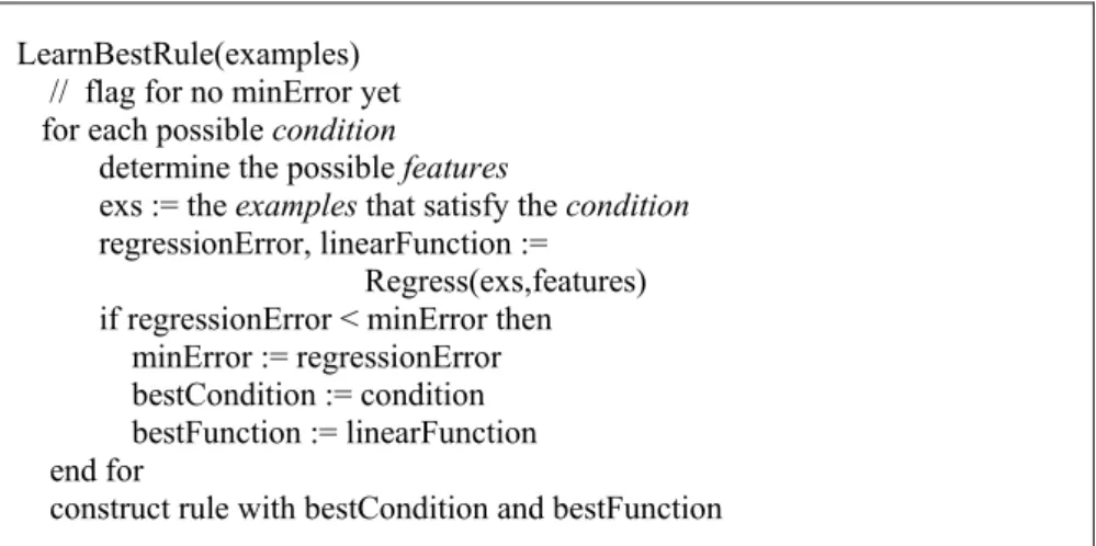
The best rule is found by trying all conditions, and deciding for the one that has associated the least error, shown in figure 6. The appropriate condition literals include all the predicates applicable in the state, and the variables are the ones found in the task, and at most one new variable for each literal in the condition. As features i.e., variables for doing the linear regression, are considered all the bound numeric variables, as well as the value functions for the subtasks of the given task.
LearnBestRule(examples) // flag for no minError yet for each possible condition
determine the possible features
exs := the examples that satisfy the condition regressionError, linearFunction :=
Regress(exs,features) if regressionError < minError then minError := regressionError bestCondition := condition bestFunction := linearFunction end for
construct rule with bestCondition and bestFunction
Figure 6: The greedy regression algorithm
6.- Learning new d-rules
In [Roncagliolo & Tadepalli, 2004] the previous described algorithm is used in order to learn the desired d-rules. Above the focus and explanation was on the value function approximation. From the d-rule point of view it can be seen as a 4-tuple <g,c,fa,vf>. Its interpretation is the following: if the goal is g, and if the condition c, which can be either one term or a conjunction of terms, is satisfied, then vf is the rule containing the value function or q-value associated to it, as explained above, and then fa is the first action that has to be taken care of. Figure 7 shows an example, it reads as follows: for the goal on(x,y), if the condition is true, in this particular case clear(y), then the q-value is obtained as indicated and the corresponding first action to be done is clear(x) .
goal: on(x,y) condition: < clear(y) > first-action: clear(x)
q-value(V): q(clear(X),_,Vl), V is V1 - 1. Figure 7: example of new d-rule
The learning algorithm has given the expected results in relation to the learned d-rules for the
blocks world. This means that given a set of examples, that include the clear, on and below
predicates the d-rules are learned as expected.
7.- Definitive form of the d-rules
Planning with these new d-rules can use the q-value in order to decide among two or more applicable d-rules, meaning that all of them are for the same goal and satisfy their respective conditions. Using these d-rules is also recursively in the sense that for a first action the process is repeated considering it the new goal.
One important difference among the d-rules is that the previous ones in its subgoal component had a sequence of subgoals to achieve or perform, allowing to consider the operator as the last element of that sequence. In contrast, in the new d-rules, first-action is only one term, thus the planning is lacking the operators itself.
Thus the proposed final d-rules have the following form: <g,c,fa,op,vf>. Their meaning remain and now has been added op, to represent the corresponding operator. Figure 8 shows the top-level algorithm. The learning of each rule remains as before, the difference is in the partition of the examples, now for learning a rule the considered examples are those that share the goal or task, the first-action or subtask and, in third place, the operator.
Learn (examples)
for each task-subtask-operator
let exs := examples for the current task-subtask-operator repeat
Rule:= LearnBestRule(Exs)
exs := exs – { ex / ex matches Rule's condition } until exs is { }
end_for
Figure 8: The top-level greedy algorithm
8.- Planning with d-rules
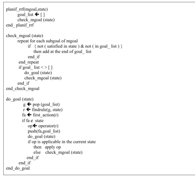
The planner needs as input a state, a goal, and a set of d-rules. The goal can be a conjunction of subgoals; the planners works with a stack of goals, and in cases with a conjunction of goals, all of them individually are placed in the stack of goals, as well as the given goal (conjunction), so at the end it is verified if it is satisfied, and in case it is not the process is repeated, until it is satisfied. Figure 9 presents the main algorithm for the planner system. The d-rules will guide the planner in what to do next at each point of the process. The value function will be the key to decide among different applicable d-rules.
9.- Results, Conclusions and Future Work
Up to this moment, we only have done preliminary experiments in the blocks world domain, allowing only one condition for each d-rule. So far, for a random generated state all examples are considered when doing the learning process. It also must be noted that not only the clear
and on predicates are used, but also the predicate below is needed in order to learn correct d-rules.
But despite what have been said, the d-rules, with their corresponding q-values are being learned as expected. Also primary results of the planner system are satisfactory. Of course
these results depend directly on the learned d-rules. Which in turn depend directly on the given examples for the learning process.
There is much that remains to be done. We need to do a bigger experimental study in the
blocks world and other domains and evaluate the algorithms more thoroughly. It appears that the condition selection can be made more efficient by adding heuristics. We assume that predicates like below are already known to the system. Introducing such useful new predicates automatically is an important open problem. Finally, we need to incorporate this algorithm into a full reinforcement learner that generates its own examples rather than being supplied with solved examples.
planif_rrf(mgoal,state) goal_list Í [ ] check_mgoal (state) end_ planif_rrf check_mgoal (state)
repeat for each subgoal of mgoal
if { not ( satisfied in state ) & not ( in goal_ list ) } then add at the end of goal_ list
end_if end_repeat if goal_ list < > [ ] do_goal (state) check_mgoal (state) end_if end_check_mgoal do_goal (state) g Í pop (goal_list) r Í findrule(g, state) fa Í first_action(r) if fa ∉ state opÍ operator(r) push(fa,goal_list) do_goal (state)
if op is applicable in the current state then apply op
else check_mgoal (state) end_if
end_if end_do_goal
Figure 9: Planning algorithm
9.- References
Blum, A. & Furst, M. (1997) Fast Planning Through Planning Graph Analysis. Artificial Intelligence, 90:281-300.
Dietterich, T. (2000). Hierarchical reinforcement learning with the maxq value function decomposition. Journal of Artificial Intelligence Research, 13, 227-303.
Džeroski, S., De Raedt, L., & Driessens, K. (2001). Relational reinforcement learning. Machine Learning, 43, 7-52.
Etzioni, O. (1993). A structural Theory of Explanation-Based Learning. Artificial Intelligence, 60(1): 93-140.
Fritz, W. (2004). Intelligent Systems and Their Societies. New Horizons Press.
Kaelbling, L. (1993). Hierarchical learning in stochastic domains: Preliminary results. Proceedings of the Tenth International Conference on Machine Learning (pp. 167-173).
Parr, R. & Russell, S. (1998). Reinforcement learning with hierarchies of machines. Advances in Neural Information Processing Systems, 10.
Quinlan, J. (1990). Learning logical definitions from relations. Machine Learning, 5, 239-266. Reddy, C. & Tadepalli, P. (2005) Learning Relational Rules for Goal Decomposition. Submitted to Machine Learning.
Reddy, C. & Tadepalli, P. (1999). Learning Horn definitions: Theory and an application to planning. New Generation Computing, 17, 77-98.
Reddy, C. & Tadepalli, P. (1997). Learning Goal-Decomposition Rules using Exercises. Proceedings of International Conference on Machine Learning (ICML).
Reddy, C., Tadepalli, P. & Roncagliolo, S. (1996). Theory-guided empirical speedup learning of goal decomposition rules. Proceedings of the 13th International Conference on Machine Learning (pp. 409-417). Bari, Italy: Morgan Kaufmann.
Roncagliolo, S. & Tadepalli, P. (2004) Function Approximation in Hierarchical Relational Reinforcement Learning. Workshop on Relational Reinforcement Learning, held in conjunction with 21st International Conference on Machine Learning, Banff, Alberta, Canada. Roncagliolo, S. (1993) Empirical Speedup Learning of Decomposition Rules for Planning. Master of Science Thesis. Department of Computer Science, Oregon State University, USA. Russell, S. & Norvig, P. (2003) Artificial Intelligence, A Modern Approach. Prentice Hall, New Jersey, USA.
Slaney, J. & Thiébaux, S. (2001) Blocks World Revisited. Artificial Intelligence 125: 19-153 Sutton, R. S., Precup, D. & Singh, S. (1999). Between mdps and semi-mdps: A framework for temporal abstraction in reinforcement learning. Artificial Intelligence, 112, 181-211.
Tadepalli P., Givan R., & Driessens K. (2004) Relational Reinforcement Learning: An Overview. Workshop on Relational Reinforcement Learning, held in conjunction with 21st International Conference on Machine Learning, Banff, Alberta, Canada.
Veloso, M., Carbonell, J., Pérez, M.A., Borrajo, D., Fink, E. &Blythe. J. (1995) Integrating planning and learning: The PRODIGY architecture. Journal of Experimental and Theoretical Artificial Intelligence 7(1):81-120.