This is an Open Access document downloaded from ORCA, Cardiff University's institutional
repository: http://orca.cf.ac.uk/123717/
This is the author’s version of a work that was submitted to / accepted for publication.
Citation for final published version:
Chen, Chong, Liu, Ying, Kumar, Maneesh, Qin, Jian and Ren, Yunxia 2019. Energy consumption
modelling using deep learning embedded semi-supervised learning. Computers and Industrial
Engineering 135 , pp. 757-765. 10.1016/j.cie.2019.06.052 file
Publishers page: https://doi.org/10.1016/j.cie.2019.06.052
<https://doi.org/10.1016/j.cie.2019.06.052>
Please note:
Changes made as a result of publishing processes such as copy-editing, formatting and page
numbers may not be reflected in this version. For the definitive version of this publication, please
refer to the published source. You are advised to consult the publisher’s version if you wish to cite
this paper.
This version is being made available in accordance with publisher policies. See
http://orca.cf.ac.uk/policies.html for usage policies. Copyright and moral rights for publications
made available in ORCA are retained by the copyright holders.
Accepted Manuscript
Energy Consumption Modelling Using Deep Learning Embedded Semi-super-vised Learning
Chong Chen, Ying Liu, Maneesh Kumar, Jian Qin, Yunxia Ren
PII: S0360-8352(19)30382-1
DOI: https://doi.org/10.1016/j.cie.2019.06.052
Reference: CAIE 5934
To appear in: Computers & Industrial Engineering Received Date: 2 January 2019
Revised Date: 4 May 2019 Accepted Date: 23 June 2019
Please cite this article as: Chen, C., Liu, Y., Kumar, M., Qin, J., Ren, Y., Energy Consumption Modelling Using Deep Learning Embedded Semi-supervised Learning, Computers & Industrial Engineering (2019), doi: https:// doi.org/10.1016/j.cie.2019.06.052
This is a PDF file of an unedited manuscript that has been accepted for publication. As a service to our customers we are providing this early version of the manuscript. The manuscript will undergo copyediting, typesetting, and review of the resulting proof before it is published in its final form. Please note that during the production process errors may be discovered which could affect the content, and all legal disclaimers that apply to the journal pertain.
Energy Consumption Modelling Using Deep Learning Embedded
Semi-supervised Learning
Chong Chena, Ying Liua*, Maneesh Kumarb, Jian Qina and Yunxia Renc
a Institute of Mechanical and Manufacturing Engineering, School of Engineering, Cardiff University, Cardiff, CF24 3AA, UK
b Institute ofService Operations, Business School, Cardiff University, Cardiff CF10 3EU, UK c National Composites Centre, Bristol & Bath Science Park, Bristol BS16 7FS, UK
*Corresponding author. E-mail: [email protected].
ABSTRACT
Reduction of energy consumption in the steel industry is a global issue where government is actively taking measures to pursue. A steel plant can manage its energy better if the consumption can be modelled and predicted. The existing methods used for energy consumption modelling rely on the quantity of labelled data. However, if the labelled energy consumption data is deficient, its underlying process of modelling and prediction tends to be difficult. The purpose of this study is to establish an energy value prediction model through a big data-driven approach. Owing to the fact that labelled energy data is often limited and expensive to obtain, while unlabelled data is abundant in the real-world industry, a semi-supervised learning approach, i.e., deep learning embedded semi-supervised learning (DLeSSL), is proposed to tackle the issue. Based on DLeSSL, unlabelled data can be labelled and compensated using a semi-supervised learning approach that has a deep learning technique embedded so to expand the labelled data set. An experimental study using a large amount of furnace energy consumption data shows the merits of the proposed approach. Results derived using the proposed method reveal that deep learning (DLeSSL based) outperforms the deep learning (supervised) and deep learning (label propagation based) when the labelled data is limited. In addition, the effect on performance due to the size of labelled data and unlabelled data is also reported.
Keywords: Energy Modelling; Intelligent Manufacturing; Deep Learning; Semi-supervised Learning; Data Mining
1. INTRODUCTION
The rapid development of the world has led to a strong demand for steel, while the steel industry faces several challenges, including decreasing natural resources, greenhouse gas emission and high energy consumption. In order to tackle these challenges, the steel industry has constantly tried to explore novel techniques for production that are sustainable, efficient and environmentally friendly. Moreover, producing steel products with better quality at a lower cost is a target of the steel industry (Delgado & Ferreira, 2010).
Recently, issues regarding environmental degradations have gained considerably increasing attention around the world. The steel industry is active in emitting greenhouse gas. According to the report from the (Commission, 2010) which analyses the carbon dioxide emission and assesses the risk of carbon leakage, the European Union endorsed a policy that aims to cut approximately 20% of the 1990 greenhouse emission levels by 2020. In the current steel industry, there are two main types of equipment for steelmaking: the basic oxygen furnace (BOF) and the electric arc furnace (EAF) (Proctor et al., 2000). Approximately one-third of the world’s steel is produced by EAF, which consumes a large sum of electricity during the steelmaking process (Yearbook, 2014). The increasing energy consumed in steelmaking process leads to more carbon dioxide emission. The industry has to reduce energy consumption to meet the requirements of strict laws and policies (Pardo & Moya, 2012). During the steelmaking process, the EAF energy consumption is mainly affected by the ingredients and process parameters. If the EAF energy consumption can be predicted based on the information of ingredients and process parameters, energy management can be optimised so as to lower the energy consumption.
The EAF energy consumption modelling can be used to predict the EAF energy consumption which can offer some insights to the steel industry (Kirschen et al., 2011; MacRosty & Swartz, 2007). The energy consumption prediction model can be built in various ways. The statistical approaches have
been used for energy modelling (Kirschen et al., 2011; Woodside et al., 1970), and they are useful when the data size is small. However, the algorithm performance could be damaged when the data size grows due to the increasing impurity and noise (Köksal et al., 2011). Recently, data mining techniques have been widely used in industrial data analytics (Veaux et al., 2016). It is also applicable in the energy consumption modelling of EAF. In the data mining field, supervised and unsupervised learning are used to tackle the labelled and unlabelled data, respectively (Mohri et al., 2012). Deep learning, as a kind of supervised learning techniques, has acquired growing attention and it is under much development in recent years. It is well known for its capacity for learning hidden patterns in data (LeCun et al., 2015). Moreover, the performance of deep learning model tends to be better when the dataset size grows, and deep learning techniques have become useful tools in data analytics (LeCun et al., 2015). However, when the data size is small, the performance of deep learning tends to be jeopardised.
In data mining field, a technique called semi-supervised learning aims to make full use of the unlabelled data for a supervised or unsupervised learning task (Hady & Schwenker, 2013). In the real world, labelled data is often expensive to be collected as it requires efforts to categorise the data. One of the critical factors which influences the supervised learning model with satisfactory performance is the size of the labelled data. When the labelled data is insufficient, it is hard to train a model with decent performance. However, with the help of unlabelled data, the performance of supervised learning algorithm could be improved (Hady & Schwenker, 2013). In semi-supervised learning, firstly, the unsupervised learning technique is used to determine the label of unlabelled data. Then the supervised learning approach is used to build a classification or regression model based on the original labelled data and the unlabelled data with new labels. The enriched data set can promote the performance of supervised learning (Zhu, 2011). Hence, introducing the semi-supervised learning technique could enable deep learning to be applicable when the labelled dataset is small.
In this work, the steel plant under investigation purchased over 20 different types of steel scraps which can be mixed in different proportions in order to get different steel products. Hence, energy
consumption in each batch of steel product differs. Currently, the statistical approaches used in the steel plant cannot deliver an accurate prediction for the EAF energy consumption per batch, which the steel plant has a keen interest in. Hence, building a reliable prediction model for EAF energy consumption is necessary. Moreover, in the context that labelled data is limited and unlabelled data is sufficient, introducing semi-supervised learning into energy consumption modelling can bring tangible benefits to the steel industry. This study aims to propose a new semi-supervised learning approach called DLeSSL which uses a small number of labelled data and a large number of unlabelled data to establish an energy consumption prediction model. In DLeSSL, firstly, we determine a rough label of the unlabelled data through unsupervised learning technique. Secondly, deep learning is introduced to compensate for the rough labels. The data assigned with the compensated label is then combined with the labelled data to an enriched dataset. The enriched dataset obtained from DLeSSL is further used for modelling using deep learning. Results indicate that deep learning based on DLeSSL performs better in energy consumption modelling. To harness the merits of deep learning in supervised learning, it requires a large sum of labelled data, which requires more efforts to obtain in the real world. However, the proposed approach enables deep learning to be performed with a small number of labelled data without sacrificing the algorithm performance dramatically (The performance decreases by approximately 8%), which is the main contribution of this study. Meanwhile, to the best of our knowledge, the existing studies in semi-supervised learning have not explored the impact of the ratio of labelled and unlabelled data on the algorithm performance. In order to reveal this pattern, this study also reported the relationship between the algorithm performance and the ratio of labelled and unlabelled data using the proposed approach. The rest of paper is organised as follows: Existing energy prediction methods of EAF, the studies of semi-supervised learning in industry, and the cases of data analytics in the industry are reviewed in Section 2. Deep learning algorithm and the proposed technique are introduced in Section 3. Section 4 introduces a case study about the modelling process using supervised and DLeSSL techniques. Results are compared and discussed in this Section to reveal the performance of DLeSSL technique. In Section 5, the benefits and limitations of DLeSSL are concluded.
2. LITERATURE REVIEW
2.1 Energy Consumption Modelling Using Statistical Methods
Energy consumption has long been a big concern for the steel industry. The energy consumption modelling can offer insights for the steelmaking process so as to be beneficial to the optimisation of the energy usage. Statistical approaches have been employed in energy modelling. In order to develop a statistical model so that the influence of the direct reduced iron on the energy balance of an EAF can be determined, several parameters regarding ingredient mass, energy conversion efficiencies and conversion of oxygen should be considered. A model based on chemical changes in the melting stage of EAF steelmaking process was designed to estimate the EAF energy efficiency. Different equations were introduced according to the chemical balance. To simplify the mass and energy conversion of the EAF melting process efficiency factors were utilized (Kirschen et al., 2011). As the efficiency factors are important in this study, how to set the factors should be further discussed.
MacRosty & Swartz (2007) proposed a mathematical framework to modify operating strategies for EAF. In this framework, a mechanistic model is incorporated using a differential-algebraic equation system to capture the dynamics of EAF processes. The model considers mass and energy balance, chemical changes and details of the EAF melting process. The hourly energy consumption was modelled in this study. In addition to the mechanistic model, a number of different mathematical procedures are used, such as Scaling equation, variable logarithmic transformations, and discontinuous approximations. These procedures are adopted in the framework to increase the robustness of the mechanistic model (MacRosty & Swartz, 2007). However, the performance of the proposed model will be jeopardised when the complexity of modelling increase, and therefore, its application will be limited.
A computer program was developed for modelling alternating current EAF energy consumption with numerous production parameters (Çamdalı & Tunç, 2002). In this program, the modelling process is based on the first law of thermodynamics. It was developed to study the effects of temperature of ingredients, such as liquid steel and stack gas, on EAF energy consumption. Different algebra equations were developed to represent the material and energy flow of EAF. The model is proposed under several assumptions such as (a) The furnace is a steady state process; (b) The EAF has a constant surface; (c) Materials going in and coming out from the EAF are uniform. In the real-life steelmaking process, it is hard to satisfy all the assumptions simultaneously, which makes this computer program hard to be applied in the actual steelmaking process.
Kaboli, Selvaraj, et al. (2016) Proposed a long-term electric energy consumption forecasting approach using artificial cooperative search algorithm. Linear, quadratic, exponential, and logarithmic model were first used to conduct the path-coefficient analysis in energy consumption modelling. Then, the artificial cooperative search algorithm is used to optimise the energy consumption prediction model. In another two cases for long-term electrical energy consumption prediction, a mathematical model was established to predict the energy consumption. Gene expression programming algorithm was adopted to optimise the model to obtain better performance (Kaboli, Fallahpour, et al., 2016; Kaboli et al., 2017).
The above cases studied energy consumption from different aspects which are chemical changes and thermodynamics. With the help of energy modelling, tasks such as energy balance and management optimisation can be achieved. Other statistical methods, such as principal component analysis, principal component regression, partial least squares and multiway modelling, have also been used for EAF energy modelling (Köhle, 2002; Sandberg, 2005). These statistical models can obtain a decent performance when the available data is clean and small in size. However, the performance of statistical model might be damaged when the size, dimension and impurity of the dataset increase.
2.2 Deep Learning and Semi-Supervised Learning in Industry
Recently, deep learning has received dramatically increasing attention and has been applied in a variety of fields (LeCun et al., 2015). As a special type of machine learning, deep learning is popularly used to identify objects in images, transcribe speech into text, and select the required data from databases (Schmidhuber, 2015). However, the application of deep learning in the industrial field is currently underdeveloped (Lu et al., 2017), with fault diagnosis being the primary application of deep learning in the industry. Gan et al. (2016) designed a hierarchical diagnosis network for fault pattern recognition of rolling element bearings. Sun et al. (2016) proposed a sparse auto-encoder-based deep neural network for motor fault classification. Li et al. (2016) developed a Gaussian-Bernoulli deep Boltzmann machine for rotating machinery fault diagnosis. Additionally, convolutional neural networks have been used for the fault identification and classification of gearbox and have also been used for fault detection in the rotating machinery (Janssens et al., 2016). All of the above cases focus primarily on rotating machinery, as it is commonly found in an industrial setting and it requires control and monitoring.
Besides being applied in fault diagnosis, a convolutional bi-directional long short-term memory network was designed to analyse the sequential data that cannot be tackled by a conventional classifier and regressor directly. In this model, the convolutional neural network is used to extract the most robust and informative features from raw data. Long short-term memory networks are adopted to extract information from sequential data, and a bi-directional structure is introduced to the long short-term memory networks so to capture the past and future contexts. Such a model can be used to predict tool wear for a CNC (computer numerical control) machine (R. Zhao et al., 2017). The above cases are the applications of deep learning in the industry. However, these applications are still limited, and most of them have focused on machine maintenance.
Meanwhile, semi-supervised learning refers to a group of techniques which can be used for modelling based on labelled and unlabelled data (Zhu, 2006). There are five main research directions within the
field of semi-supervised learning: generative model (Baluja, 1999; Nigam et al., 2000) which is based on the generative assumption, self-training model (Rosenberg et al., 2005; Yarowsky, 1995) which adds the unlabelled sample to the model to improve performance, co-training model (Blum & Mitchell, 1998; Zhan & Zhang, 2017) which co-trains two models simultaneously, avoiding changes in dense regions (Chapelle et al., 2008) which aims to find the low data density regions , and graph-based methods (Blum & Chawla, 2001; Talukdar & Pereira, 2010) which is originated from label propagation algorithm (Zhu & Ghahramani, 2002) and can be used to extract class-instance pairs from large unstructured and structured dataset. These techniques have all been applied to tackle different real-world problems. Despite this, the application of semi-supervised learning in the industry remains limited.
When the available labelled data is limited, establishing a classification model with decent performance tends to be hard. Ge et al. (2016) proposed a kernel-driven semi-supervised Fisher discriminant analysis (FDA) model for nonlinear fault classification. The proposed method uses a semi-supervised data matrix and FDA technique to extract the discriminant information, before k -nearest neighbours and Bayesian techniques were used for classification. The size of labelled data used in this case was 400, and there were 41 attributes in the dataset, with a ratio of labelled data to unlabelled data is 1:1. Zhou et al. (2014) proposed a semi-supervised probabilistic latent variable regression method to improve the performance monitoring of variations in the process and the features relevant to the product quality. The probabilistic latent variable regression approach was used for modelling, and an EM (Expectation Maximisation) algorithm was used to estimate the parameters of the semi-supervised model. In this case, 50 labelled instances and 450 unlabelled instances were utilised for model building. The performance of a probabilistic latent variable regression model is the sole benchmark in this case, which makes it difficult to reveal the advantages of the proposed method compared to other approaches. M. Zhao et al. (2017) proposed a semi-supervised model with a capped
l2,1-norm regularisation. A loss term was used to measure the inconsistency between the prediction and the original labels to the labelled dataset. A global regression regularised term was developed to train a classification model which can achieve better performance. However, the size of the labelled
and unlabelled data was not mentioned in this case. Kang et al. (2016) proposed a semi-supervised support vector regression (SS-SVR) method based on self-training and applied it to virtual metrology in a semiconductor manufacturing context. The distribution of labels for the unlabelled data was estimated by a probabilistic regression model, and the support vector machine algorithm was used to build the regression model. The data of semi-conductor manufacturing was collected from the sensors embedded in process equipment and previous metrology values. SS-SVR can achieve better prediction accuracy and efficiency compared to the conventional support vector regression. The combined quantity of the labelled and unlabelled data was over 60,000 in this study, and the labelled data make up approximately 6% in this total.
Such semi-supervised cases mentioned above have demonstrated that a better modelling performance can be achieved with the help offered by unlabelled data. However, none of the presented studies has assessed the impact of the different ratios of labelled and unlabelled data on performance. Moreover, there have been no state-of-the-art applications of semi-supervised learning in the steel industry.
2.3 Machine Learning in the Steel Industry
Approximately one-third of the world’s steel is currently being produced using the EAF steelmaking process (Mohsen & Akash, 1998), and there are a variety of factors that may influence different aspects of it; including scrap price, the molten steel temperature, and electrode voltage, etc. Despite the highly specialised empirical knowledge which engineers in the steel industry possess (Fernández et al., 2008), when a problem in the actual process is affected by numerous factors, finding solutions using empirical knowledge and traditional statistical methods can be challenging. Data mining, which extracts knowledge from a complex dataset, has gained growing attention in the manufacturing sector (Veaux et al., 2016). Machine learning provides the technical basis of data mining (Witten et al., 2016). As a useful tool in data mining, machine learning can be used to find the hidden patterns which are helpful to the steel industry.
Several linear regression models have been used to determine the energy balance of EAF and the relationship among different parameters in EAF. These parameters include the energy input and energy efficiency, natural gas enthalpy and electrical energy requirement (Kirschen et al., 2009). Fernández et al. (2008) proposed a mixed model consisting of a fuzzy inference function and an artificial neural network to predict the tap temperature of the EAF. In this study, an artificial neural network was used for classification, and the fuzzy inference function was adopted to generate the final tap temperature. In order to predict the gas consumption in a steel plant, Kovačič & Šarler (2014) investigated a model based on genetic programming. The genes used in this case can be categorised into two types: terminal genes which are the variables in the steelmaking process; and function genes which are the operation rules (i.e., addition, subtraction, multiplication and division). After the random generation of the program tree and the crossover process was repeated, the prediction model with the best performance was found. As the physical model is deficient in predicting and controlling the temperature of molten steel in a tundish during a continuous casting process, a grey box model was established by combining a first-principle model and a statistical model (Ahmad et al., 2014). The first-principle model was used to model the linear and nonlinear relations in the dataset, and a mathematical model is used for extracting the unknown ties from the data. In the end, a random forest algorithm was applied to the statistical model as an ensemble classifier. The above cases indicate machine learning techniques have been used in the steel industry for different purposes. However, relevant studies using machine learning in energy consumption modelling is still limited.
The steel plant being investigated in this study uses a Microsoft Excel-based software call solver to establish the best combination of different scraps, energy consumption and outputs, based on the values of specific parameters which are input by engineers. This dataset contains the information of ingredients (i.e. scraps and additives) and processing parameters, including some impurity as well. The application of statistical method is not advantageous, as it has strict requirements with regards to the input dataset. Moreover, it has to be cleaned and low in impurity, and the large size and dimensions of the dataset may damage the modelling performance of statistical approach. As
previously mentioned, deep learning, as a machine learning algorithm, is currently widely applied in different fields, and it is a useful tool in building models with a high dimensional and large size dataset. In our previous study, we introduced deep learning into energy consumption modelling. The experimental results indicated that deep learning shows merits in energy consumption modelling in comparison with several machine learning algorithms (Chen et al., 2018). However, to the best of our knowledge, all the state-of-the-art energy modelling methods are based on supervised learning techniques, despite labelled data being expensive and hard to obtain in the real world when compared with unlabelled data (Zhu, 2011). Since semi-supervised learning techniques aim for modelling based on the small size of labelled data (Zhu, 2011), it is a potentially useful tool in energy modelling when the labelled data is insufficient and the unlabelled data is abundant.
3. DEEP LEARNING EMBEDDED SEMI-SUPERVISED
LEARNING: ALGORITHM AND APPROACH
In this work, a new approach called deep learning embedded semi-supervised learning (DLeSSL) is proposed to help energy modelling based on a small number of labelled data and a large number of unlabelled data. In this approach, deep learning is embedded into semi-supervised learning algorithm to improve its performance. In Section 3.1, the design procedure of deep learning model is introduced and how deep learning is embedded into semi-supervised learning is detailed in Section 3.2.
3.1 The Design of Deep Learning Models
Deep learning is a neural network-based technique that contains a large number of hidden layers for discovering the hidden knowledge from data (LeCun et al., 2015). It is a highly interconnected system that consists of an input layer, hidden layers and an output layer. Each layer is made up of plentiful hidden neurons, which is collectively known as nodes.
There are several types of existed deep learning models, with expertise in carrying out different tasks and process different types of data. The prediction of energy consumption is based on the data of raw materials and process parameters of EAF, which can be handled by fully connected layers. There are mass neurons in a fully connected layer, which offer a powerful computational ability. Hence, a deep neural network, which consists of multi-fully connected layers, is adopted. It is trained using backpropagation algorithm, which is used to the determine weight and bias of the neural network (LeCun et al., 2015). The design of a deep learning model needs to determine the necessary elements, which are the type of layer, activation function, loss function and optimiser. In order to build a prediction model, all the elements need to be well considered according to their properties and the characteristics of the data.
Firstly, the type of layer needs to be selected according to the characteristics of data. The type of layer is determined by the type of data. For instance, a recurrent layer is suitable for dealing with sequential data, and a convolutional layer is good at tackling image data (Schmidhuber, 2015). Secondly, there are several different types of activation functions, loss functions and optimisers. The selection of these elements is highly data dependent. In order to get optimal performance, they need to be tested and finetuned using the actual data.
Meanwhile, another issue that needs to be considered is that there is no explicit guideline for the determination of the number of nodes and hidden layers because these parameters are highly data dependent. First, the number of nodes in each layer should be the same as it can yield better performance than the pyramid-like node setting (Bergstra & Bengio, 2012). Secondly, a larger number of nodes and hidden layers result in a large computational load. When the number of nodes and hidden layers are insufficient, the model may not able to learn enough hidden patterns. Hence, they need to be determined in the actual case.
3.2 Deep Learning Embedded Semi-supervised Learning
Notations
I The total number of labelled data
J The total number of unlabelled data
Instance in labelled dataset
�� ��∈{��, …, ��}
The labels of the instances in labelled dataset,
�� ��∈{��, …,��}
Instance in unlabelled dataset
�� ��∈{��, …, ��}
The most similar for ,
�� �� �� ��∈{��, …, ��}
The new label of ,
�� �� ��∈{��, …,��}
Bias between new label and the actual label of ,
∆�� �� �� ∆��∈{∆��, …,∆��}
Difference of and ,
∆�� �� �� ∆��∈ {∆��, …, ∆��}
Difference of each two , ,
∆�� �� ∆��∈{∆��, …,∆��} �=�(� ‒ �)�
Difference of each two , ,
∆�� �� ∆��∈{∆��, …,∆��} �=�(� ‒ �)�
The compensated label of
�� �� ��∈{��, …��}
We assume that there are a labelled dataset and an unlabelled dataset. The size of the unlabelled dataset is significantly larger than that of the labelled dataset. If the labelled data is insufficient to train a model with a decent performance, exploiting the unlabelled data emerges as an available option to improve the algorithm performance. Different kinds of supervised learning algorithms have been introduced for energy modelling for the steel industry. Such tools show advantages on building the prediction model based on labelled data. However, when the labelled data is insufficient, the performance of supervised learning approach tends to be unsatisfactory.
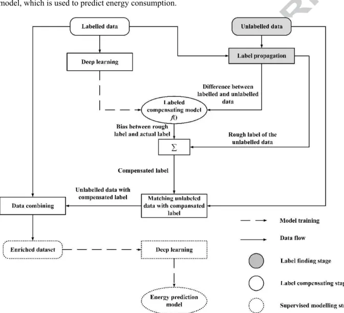
In order to improve the algorithm performance when the labelled data is limited DLeSSL was proposed. The general flow of DLeSSL is shown in Fig. 1. The proposed approach can be separated into two stages i.e. the label finding stage and the label compensating stage. The label finding stage is
originated from label propagation algorithm (Zhu & Ghahramani, 2002). In the label finding stage, new labels of the unlabelled data are determined. In the label compensating stage, the new labels are compensated using deep learning technique. When the compensated labels of the unlabelled data are obtained, the labelled data and the unlabelled data with the compensated label are combined as an enriched dataset. The enriched dataset obtained from DLeSSL is used to train a new deep learning model, which is used to predict energy consumption.
Fig. 1. The flow chart of DLeSSL
The label finding stage aims to identify the labels for the unlabelled data. Firstly, the most similar labelled instances for the unlabelled data is determined. In this case, we have adopted radial basis function (RBF) to determine the similarity between two instances base on its performance and convenience (Vert et al., 2004). The RBF is used to represent the similarity or distance between ��and
. When the close to zero, it indicates the similarity between the label instance and the
�� ��� (��,��) ��
unlabelled instance ��is considerably high. An RBF is denoted as:
(1) ��� (��,��) =���
(
‒�(��,��)2 2�2
)
where σ is a parameter of RBF and is the Euclidean distance.�
Secondly, label propagation is carried out based on the ��� (��,��), which means the most similar instance �� for �� will be found. Then, the label of �� is propagated to ��. The details of the label propagation algorithm can be found in the work of (Zhu & Ghahramani, 2002). Basically, when �� is known and ��is unidentified, ��can be considered approximately equal to ��. The label propagation process can be represented as:
=> = (2)
(��,��)→(��) (��,��) (��,��)
However, even ��is the most similar instance for ��in the labelled dataset, it does not mean the new label ��is equal to the actual label of ��. There is still a slight difference between ��and ��. In order to get close to the actual label of ��, compensation to �� need to be carried out. In this stage, �� is unknown and the bias ∆�� between new label ��and the actual label of �� is estimated in the next stage.
In the label compensating stage, we model the relationship between ∆�� and ∆�� by utilising deep learning technique due to its excellent performance in data analytics (LeCun et al., 2015). The number of ∆�� is �=�(� ‒ �)� , which grows rapidly when the number of label data increases. The model which is used to represent the relationship between ∆��and ∆�� can be modelled using deep learning algorithms. It can be denoted as:
∆��=�(∆��) (3)
After the label compensating model �() is obtained, it can be used to determine the bias ∆��. In the label compensating model �() ∆�, �is used as the input of �() to yield ∆��, which can be denoted as:
(4) ∆��=�(∆��)
Finally, with the new label ��and the bias ∆��, the compensated label is denoted as:��
(5)
��=��+ ∆��
When the new label ��is obtained, the unlabelled data and the label data is combined as an enriched dataset. The enriched dataset yielded by DLeSSL is then used to build a deep learning model to predict energy consumption.
After the prediction models are established, algorithm performance is mainly evaluated by model correlation coefficient (MCC) (Taylor, 1997). MCC is used to represent the similarity between two variables. In this study, MCC is used to measure the similarity between a predicted value and its corresponding actual value. It can be denoted as:
, (6) MCC = ���� ��� where, ���=
∑
�(
��‒ �)(
��‒ �)
� ‒1 ; ��=∑
�(��‒ �)2 � ‒1 ; ��=∑
�(��‒ �)2 � ‒1 ;is the predicted value and is the average of the predicted value. is the actual value and the is
�� � �� �
the average actual value. is the number of the training data.�
4. CASE STUDY
The understanding of a steelmaking process is essential to process modelling. The first step in the steelmaking process is adding the collected scraps and additive into EAF. Then, the scraps are melted, before the impurity of the scraps is removed with the help of additive. The next stage is carbon adjustment where carbon is injected to meet the required carbon content in steel. In the final stage, steel products, such as plate and tube, are obtained after hot rolling and casting process.
In our study, the dataset was collected from the melt shop in an established steel plant in South Wales, UK. The steel plant uses a data-management software called System Analysis and Program Development to record and upload data to a cloud drive. The data collected from the steel plant has 40 attributes and 10,987 instances. The attributes in the dataset can be categorised into seven groups according to their properties. Table 1 shows the results of attributes classification.
Table 1.
The classification of attributes.
Category Attribute
Scraps Clean bales 1, Clean bales 2, Merchant 1 & 2, Tin Can, Estructural, Fragmentized scrap, Steel
turnings, Recovered Scrap, Total Scrap Mix
Additive Main Oxygen, Secondary Oxygen, Natural Gas, Carbon injected, Lime, Dolomite
Index Heat Number
Nominal Steel Grade
Power
Average power LEVEL 2, PON time (min), TTT Level 2, Power factor, Apparent Power, Reactive Power, Current/kA, Foaming Index, Primary Volts (Onload), Varc
Temperature T TAP (ºC), TLF entry (ºC), Ladle Energy Cons (KWh), PRECIPITATION (mm), Temperature (ºc)
Pressure Average of cb1oxymainpressure, Average of cb2oxymainpressure, Average of cb3oxymainpressure
Output EAF (MWh), Billet Tons
4.2 Feature Selection and Data Pre-processing
Feature selection aims to improve the performance and generalisation ability of data mining algorithms to reduce computation load and to provide a deeper understanding of features in the
problem domain (Guyon & Elisseeff, 2003). In this study, firstly, features such as scraps and additives that are directly related to the energy consumption of EAF are adopted. EAF (MWh) is the target variable (i.e. energy consumption of EAF) in this case. Secondly, other attributes, whose relationship to the energy consumption is hard to determine, are analysed by an attribute selection algorithm in the Weka software (Hall et al., 2009). The algorithm deployed in this case is CfsSubEval, and it contains two strategies: BestFirst (Xu et al., 1988) and GreedyStepwise (Caruana & Freitag, 1994). The results of different strategies are very similar. Table 2 shows the results of the feature selection.
Table 2.
The result of feature selection.
Note relevancy is a metric that reveals the correlation between the listed attributes and energy consumption. A higher relevancy indicates that attribute is more relevant to the energy consumption. The results of feature selection indicate that PON time (min), TTT level 2, Primary Volts (Onload) and
Average of cb1oxymainpressure are more related to the energy consumption of EAF. However, there are 49% and 16% missing values in Primary Volts (Onload) and Average of cb1oxymainpressure, respectively. Since it is very often the case that a large percentage of missing values will jeopardise the performance during model building, Primary Volts (Onload) and Average of cb1oxymainpressure were not selected. Hence, including PON time (min) and TTT level 2, there are in total of 17 features
Attribute Relevancy Attribute Relevancy
Heat Number 0% Primary Volts (Onload) 100%
Billet Tons 0% Varc 0%
Average power LEVEL 2 0% Secondary Oxygen 0%
PONtime (min) 100% T TAP (ºC) 0%
TTT Level 2 10 % TLF entry (ºC) 0%
Power factor 0% Ladle Energy Cons (kwh) 0%
Apparent Power 0% PRECIPITATION (mm) 0%
Reactive Power 0% Temperature (ºc) 0%
Current/kA 0% Average of cb1oxymainpressure 10%
Foaming Index 0% Average of cb2oxymainpressure 0%
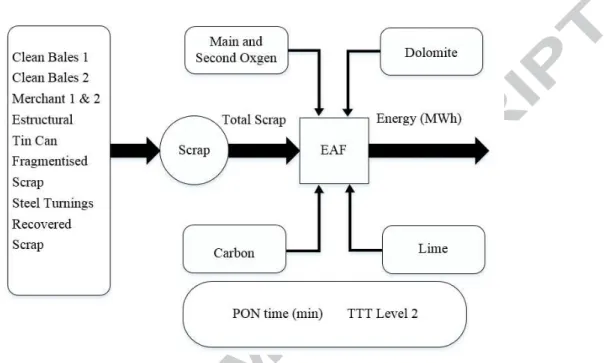
that were selected to establish an energy consumption model. Fig.2 shows the EAF modelling using the selected features.
Fig. 2. EAF modelling process using the selected features
The dataset was pre-processed before it was input for modelling. Firstly, abnormal values need to be replaced. The statistical distribution of most features is Gaussian except for Dolomite. Approximately 80% of the instances in Dolomites are located near 800 kg, while the rest of the instances are discrete from 0 kg to 7,000 kg. There are approximately 1% of instances from Dolomite are over 7,000 kg, since domain expertise says it is not reasonable to add that much Dolomites into the EAF, hence, those values were replaced by the most frequent values. Secondly, approximately 3% of instances have missing values of Second oxygen, Main oxygen, Natural gas and Carbon injected. This is likely due to sensor failures. Because the missing values of the other attributes make up about approximately 0.05% of the dataset, it is difficult to estimate all the missing values precisely. Hence, instances which contain these missing values were deleted. the number of the remaining instances in the dataset was 10,710. Thirdly, the data were normalised to reduce data redundancy and enhancing data integrity. Finally, randomisation was implemented. In the dataset, each instance is an EAF processing record, and the record was uploaded to the database chronologically. To avoid local hidden patterns which
cannot represent global characteristics of EAF, all 10,710 data entries were randomised. After the data pre-processing stage, the dataset was brought forward to establish a prediction model for EAF energy consumption.
4.4 Energy Consumption Modelling Using Deep Learning
In our previous study, deep learning and several prevailing machine learning algorithms (linear regression, support vector machine, and decision tree) were used for energy modelling. The results of the previous study are shown in Table 3. It can be seen from the results that the performance of deep learning in terms of MCC, mean absolute error (MAE) and maximum error (MaxE) is better than the prevailing machine learning algorithms (Chen et al., 2018). Because deep learning shows merits in comparison with the prevailing machine learning algorithms, it was selected to establish an energy consumption model based on the data obtained from DLeSSL in this study.
Table 3.
The comparison of the MCC, MAE, MaxE.
Metrics Deep learning Linear regression Support vector
machine Decision tree
Model Correlation coefficient (MCC) 0.854 0.785 0.762 0.775 Mean Absolute Error (MAE) 1.254 2.103 1.709 1.946 Maximum Error (MaxE) 17.362 25.211 26.226 29.491
The parameters of deep learning are set as follows. Firstly, the deep learning structure used in this case is a deep neural network, which consists of full connected layers. The number of layers and neurons needs to be considered with the computational load and algorithm performance. After several different trials, the number of hidden layers was set at four and neurons in each layer was set at 500. ReLU (Rectifier Linear Unit), a prevailing activation function, was selected for the input and hidden layers ("Keras Documentation," 2016). Adam, a prevailing optimiser, is widely used in the deep learning field due to its excellent performance, and therefore it was used to build a regression model (Kingma & Ba, 2014). In order to measure the compatibility between predicted values and their
corresponding actual values in deep learning, a loss function is necessary. Due to its wide application in prediction, the mean square error was adopted as the loss function.
4.4 Energy Consumption Modelling Using DLeSSL
In this stage, DLeSSL was introduced into our study to label the unlabelled data. There are two purposes in this section. On the one hand, in what extent DLeSSL can be beneficial the algorithm performance using a small size of labelled data and a large size of unlabelled data needs to be determined. On the other hand, what is the suitable range for the ratio of labelled data and unlabelled data for DLeSSL needs to be investigated.
DLeSSL is composed of two stages: label finding stage and label compensating stage. As deep learning is used in DLeSSL, its parameters need to be well considered. The setting of deep learning used in label compensating stage is basically the same as the deep learning model mentioned in Section 4.3, except the activation function and the size of the nodes in each layer. After trails, linear function was adopted as the activation function in label compensating model as there are both positive and negative values in input data. Meanwhile, the number of nodes was reduced to 200.
Because deep learning achieved the best performance in terms of MCC, MAE, and MaxE in energy consumption modelling in our previous study, it was used for energy consumption modelling in this study. Meanwhile, 5-fold cross-validation was implemented. MCC was used as the only metric to reveal the performance of different algorithms.
In this study, only a small part of the instances in the dataset were selected as labelled data. The size of labelled instances was set at different values in the range from 50 to 1000. The rest instances in the dataset were used as unlabelled data, which labels were removed. In the modelling stage, after the compensated labels of the unlabelled data were obtained, the labelled data was combined with the
unlabelled data with the compensated labels to an enriched dataset, which was used to train an energy consumption prediction model using deep learning. In order to reveal the performance of DLeSSL, a deep learning algorithm based on label propagation algorithm was adopted as a baseline. Meanwhile, a deep learning algorithm using a small size of labelled data was also adopted as a baseline. It is denoted as deep learning (supervised). Label propagation algorithm is a semi-supervised learning algorithm that used to determine the label of unlabelled data (Zhu & Ghahramani, 2002).
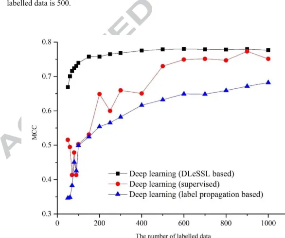
Fig. 4 shows the relation between the number of labelled data and the MCC of deep learning based on different algorithms, where the x-axis represents the number of labelled data and the y-axis represents MCC. It can be seen that the performance of the deep learning (DLeSSL based) in terms of MCC is the highest in every stage. Starting at 0.679, there is a dramatic increase in performance when the number of labelled data increased from 50 before it remains steady after 200. The highest performance of the deep learning (DLeSS based) in terms of MCC is 0.780, where the number of labelled data is 500.
Fig. 4. The relation between the number of the labelled data and the MCC of deep learning based on different semi-supervised learning algorithms
In the meantime, the performance of deep learning (supervised) and deep learning (label propagation based) in terms of MCC are lower than that of deep learning (DLeSSL based). The performance of the deep learning (supervised) in terms of MCC fluctuated in all stages with the overall trend is upward. Increasing from 0.515, the performance of deep learning (supervised) in terms of MCC experienced a striking fluctuation when the number of labelled data range from 50 to 100. The highest performance of deep learning (supervised) in terms of MCC is 0.772, where the number of labelled data is 900. The peak performance of deep learning (supervised) in terms of MCC is close to that of deep learning (DLeSSL based). The performance of deep learning (label propagation based) in terms of MCC is the worst in most of the stages. Meanwhile, rsing from 0.346, there is a sharp increase in the performance of deep learning (label propagation based) in terms of MCC to 0.499 where the number of labelled data is 100. When the number of labelled data is situated in the range from 150 to 1000, the performance of deep learning (label propagation based) in terms of MCC is upward, with the highest MCC situating at 0.6823. It is obvious that the growing trend of deep learning (DLeSSL based) and deep learning (label propagation based) are more stable in comparison with deep learning (supervised). Meanwhile, the performance of deep learning (supervised) and deep learning (label propagation based) in terms of MCC are likely upward when the number of labelled data exceed 1000.
It also can be seen from Fig. 4 that when the number of labelled data is over 150, the performance of deep learning (DLeSSL based) in terms of MCC tends to converge. It is 0.758 when the number of the labelled data is 150, which is slightly lower than the optimal performance which is 0.780. Moreover, when the number of labelled data range from 150 to 600, deep learning (DLeSSL based) shows merits. In contrast, when the labelled data increases to 600, the difference in performance in terms of MCC between deep learning (DLeSSL based) and deep learning (supervised) is not considerable, which means deep learning (DLeSSL based) does not show advantages in comparison with the other two algorithms. Hence, the range of labelled data between 150 to 600 can be deemed as a suitable range
for DLeSSL. The unlabelled data used in this case is 7,568. The suitable range for the ratio of labelled data and unlabelled data is 1.982% to 7.923% for DLeSSL algorithm.
4.5 Discussion
Due to energy consumption has become a big concern in the steel industry, the proposed approach can be deployed in the steel industry to achieve better energy management. With an energy prediction model established using the proposed approach when the labelled data is insufficient, the impact of ingredients and process parameters on energy consumption can be identified. The prediction of energy consumption can be obtained by feeding formula and process parameters into the energy consumption prediction model. After different trials, the optimum formula which can lower energy consumption without compromising the steel quality can be determined.
It is noticeable from the results that when the data size is insufficient, deep learning shows poor performance in terms of MCC. Also, the performance of deep learning tends to be unstable when the data size is small, which can be seen from the fluctuated trend of deep learning (supervised). The experimental results demonstrate that the performance of the deep learning (DLeSSL based) is better than deep learning (supervised). In striking contrast, the performance of deep learning (label propagation based) is lower than that of the deep learning (supervised), which indicate that label propagation algorithm damages the performance of deep learning in this case. This may be caused by the labels obtained using label propagation algorithm (Zhu & Ghahramani, 2002) are inaccurate. With the inaccurate label, the unlabelled data becomes noise in the dataset and therefore jeopardise the performance of deep learning. Hence, the experimental results indicate that DLeSSL can be a useful tool in energy consumption modelling. In this case, the best MCC of the deep learning (DLeSSL based) is 0.780, which is lower than the MCC of 0.854 for the deep learning in our previous study. The difference in performance is caused by the bias between the compensated label obtained by the proposed approach and the actual label of the unlabelled data. With the application of the proposed
technique, the required quantity of labelled data can be reduced by over 90% with the performance sacrificing by approximately 8%.
To the best of our knowledge, most of the existing efforts in semi-supervised learning have tended to investigate the algorithm performance. However, the deployment of semi-supervised learning also needs to be studied. The identification of the relationship between the ratio and performance can be beneficial to the deployment of semi-supervised approach in the actual case. In this case, we determined the suitable range from 1.982% to 7.923%. This insight can be helpful in the deployment of DLeSSL in the actual case. Moreover, DLeSSL is used to find and compensate the label of the unlabelled data. By using this method, unlabelled data can be used to help the supervised learning task. Several existing semi-supervised learning algorithms only use unsupervised learning method to determine the label for unlabelled data. Different from the existing efforts, both unsupervised learning (label finding) and supervised learning (label compensating) are used in DLeSSL to determine the label of unlabelled data. In the future, the difference between the proposed approach and the existing semi-supervised learning algorithms will be studied to further reveal the performance of DLeSSL and find potential ways to improve it.
5. CONCLUSIONS
The steel industry has a keen interest in reducing energy consumption. In this paper, the focus is on the modelling and prediction of energy consumption given an example of EAF in the steel industry. With an accurate energy consumption prediction model, the steelmaking formula and process parameters can be optimised to lower energy consumption. Relevant works, e.g., computational modelling techniques of EAF, research on semi-supervised learning, deep learning and data analytics in the steel industry, were reviewed. Based on deep learning and label propagation algorithms, a new semi-supervised approach called DLeSSL (deep learning embedded semi-supervised learning) for energy consumption modelling using a small size of labelled data and a large size of unlabelled data
was proposed. Different from the existing efforts that use unsupervised learning algorithm to determine the label of unlabelled data, DLeSSL uses both unsupervised and supervised learning algorithm to label the unlabelled data. This approach consists of two stages: the label finding and the label compensating stage. The aim of DLeSSL is to determine and compensate the labels of unlabelled data using deep learning technique. Thereafter, the new dataset yielded by DLeSSL is used to train a deep learning model to predict the energy consumption of EAF. A case study is carried out using real-world EAF data. The results have shown the merits of the proposed approach. Experimental results also have indicated that with the help of DLeSSL, deep learning tends to yield better performance when labelled data is scarce. Meanwhile, our finding highlights the suitable range for the ratio of labelled and unlabelled data in this study, which can offer insights to the actual deployment of the proposed approach. In the steel industry, DLeSSL can be a useful tool in energy consumption modelling when labelled data is limited.
REFERENCES
Ahmad, I., Kano, M., Hasebe, S., Kitada, H. & Murata, N. (2014). Gray-box modeling for prediction and control of molten steel temperature in tundish. Journal of Process Control, 24(4), 375-382. Baluja, S. (1999). Probabilistic modeling for face orientation discrimination: Learning from labeled
and unlabeled data. In: Advances in Neural Information Processing Systems (pp. 854-860). Bergstra, J. & Bengio, Y. (2012). Random search for hyper-parameter optimization. Journal of
Machine Learning Research, 13(Feb), 281-305.
Blum, A. & Chawla, S. (2001). Learning from labeled and unlabeled data using graph mincuts.
Blum, A. & Mitchell, T. (1998). Combining labeled and unlabeled data with co-training. In: Proceedings of the eleventh annual conference on Computational learning theory (pp. 92-100): ACM.
Çamdalı, Ü. & Tunç, M. (2002). Modelling of electric energy consumption in the AC electric arc furnace. International Journal of Energy Research, 26(10), 935-947.
Caruana, R. & Freitag, D. (1994). Greedy attribute selection. In: Machine Learning Proceedings 1994 (pp. 28-36): Elsevier.
Chapelle, O., Sindhwani, V. & Keerthi, S.S. (2008). Optimization techniques for semi-supervised support vector machines. Journal of Machine Learning Research, 9, 203-233.
Chen, C., Liu, Y., Kumar, M. & Qin, J. (2018). Energy Consumption Modelling Using Deep Learning Technique—A Case Study of EAF. Procedia CIRP, 72(1), 1063-1068.
Commission, E.-E. (2010). Analysis of options to move beyond 20% greenhouse gas emission reductions and assessing the risk of carbon leakage. Commission Staff working document, SEC (2010), 650.
Delgado, C. & Ferreira, M. (2010). The implementation of lean Six Sigma in financial services organizations. Journal of Manufacturing Technology Management, 21(4), 512-523.
Fernández, J.M.M., Cabal, V.Á., Montequin, V.R. & Balsera, J.V. (2008). Online estimation of electric arc furnace tap temperature by using fuzzy neural networks. Engineering Applications of Artificial Intelligence, 21(7), 1001-1012.
Gan, M., Wang, C. & Zhu, C.a. (2016). Construction of hierarchical diagnosis network based on deep learning and its application in the fault pattern recognition of rolling element bearings. Mechanical Systems and Signal Processing, 72-73, 92-104.
Ge, Z., Zhong, S. & Zhang, Y. (2016). Semisupervised kernel learning for FDA model and its application for fault classification in industrial processes. IEEE Transactions on Industrial Informatics, 12(4), 1403-1411.
Guyon, I. & Elisseeff, A. (2003). An introduction to variable and feature selection. Journal of Machine Learning Research, 3(Mar), 1157-1182.
Hady, M.F.A. & Schwenker, F. (2013). Semi-supervised learning. In: Handbook on Neural Information Processing (pp. 215-239): Springer.
Hall, M., Frank, E., Holmes, G., Pfahringer, B., Reutemann, P. & Witten, I.H. (2009). The WEKA data mining software: an update. ACM SIGKDD explorations newsletter, 11(1), 10-18.
Janssens, O., Slavkovikj, V., Vervisch, B., Stockman, K., Loccufier, M., Verstockt, S., Van de Walle, R. & Van Hoecke, S. (2016). Convolutional Neural Network Based Fault Detection for Rotating Machinery. Journal of Sound and Vibration, 377, 331-345.
Kaboli, S.H.A., Fallahpour, A., Kazemi, N., Selvaraj, J. & Rahim, N. (2016). An expression-driven approach for long-term electric power consumption forecasting. American Journal of Data Mining and Knowledge Discovery, 1(1), 16-28.
Kaboli, S.H.A., Fallahpour, A., Selvaraj, J. & Rahim, N. (2017). Long-term electrical energy consumption formulating and forecasting via optimized gene expression programming. Energy, 126, 144-164.
Kaboli, S.H.A., Selvaraj, J. & Rahim, N. (2016). Long-term electric energy consumption forecasting via artificial cooperative search algorithm. Energy, 115, 857-871.
Kang, P., Kim, D. & Cho, S. (2016). Semi-supervised support vector regression based on self-training with label uncertainty: An application to virtual metrology in semiconductor manufacturing. Expert Systems with Applications, 51(Supplement C), 85-106.
. Keras Documentation. In. (2016).
Kingma, D. & Ba, J. (2014). Adam: A method for stochastic optimization. arXiv preprint arXiv:1412.6980.
Kirschen, M., Badr, K. & Pfeifer, H. (2011). Influence of direct reduced iron on the energy balance of the electric arc furnace in steel industry. Energy, 36(10), 6146-6155.
Kirschen, M., Risonarta, V. & Pfeifer, H. (2009). Energy efficiency and the influence of gas burners to the energy related carbon dioxide emissions of electric arc furnaces in steel industry. Energy, 34(9), 1065-1072.
Köhle, S. (2002). Recent improvements in modelling energy consumption of electric arc furnaces. In: Proc. 7. Europ. Electric Steelmaking Conf., Venedig, Italien (Vol. 26, pp. 29).
Köksal, G., Batmaz, İ. & Testik, M.C. (2011). A review of data mining applications for quality improvement in manufacturing industry. Expert Systems with Applications, 38(10), 13448-13467.
Kovačič, M. & Šarler, B. (2014). Genetic programming prediction of the natural gas consumption in a steel plant. Energy, 66, 273-284.
LeCun, Y., Bengio, Y. & Hinton, G. (2015). Deep learning. Nature, 521(7553), 436-444.
Li, C., Sánchez, R.-V., Zurita, G., Cerrada, M. & Cabrera, D. (2016). Fault diagnosis for rotating machinery using vibration measurement deep statistical feature learning. Sensors, 16(6), 895. Lu, C., Wang, Z. & Zhou, B. (2017). Intelligent fault diagnosis of rolling bearing using hierarchical
convolutional network based health state classification. Advanced Engineering Informatics,
32, 139-151.
MacRosty, R.D. & Swartz, C.L. (2007). Dynamic optimization of electric arc furnace operation. AIChE journal, 53(3), 640-653.
Mohri, M., Rostamizadeh, A. & Talwalkar, A. (2012). Foundations of machine learning: MIT press. Mohsen, M.S. & Akash, B.A. (1998). Energy Analysis of the Steel Making Industry. International
Journal of Energy Research, 22, 1049-1054.
Nigam, K., McCallum, A.K., Thrun, S. & Mitchell, T. (2000). Text classification from labeled and unlabeled documents using EM. Machine Learning, 39(2), 103-134.
Pardo, N. & Moya, J.A. (2012). Prospective scenarios on energy efficiency and CO2 emissions in the EU iron & steel industry (Vol. 54). Luxembourg: Publications Office of the European Union.
Proctor, D., Fehling, K., Shay, E., Wittenborn, J., Green, J., Avent, C., Bigham, R., Connolly, M., Lee, B. & Shepker, T. (2000). Physical and chemical characteristics of blast furnace, basic oxygen furnace, and electric arc furnace steel industry slags. Environmental science & technology,
34(8), 1576-1582.
Rosenberg, C., Hebert, M. & Schneiderman, H. (2005). Semi-supervised self-training of object detection models.
Sandberg, E. (2005). Energy and scrap optimisation of electric arc furnaces by statistical analysis of process data. Luleå tekniska universitet.
Schmidhuber, J. (2015). Deep learning in neural networks: An overview. Neural Networks, 61, 85-117.
Sun, W., Shao, S., Zhao, R., Yan, R., Zhang, X. & Chen, X. (2016). A sparse auto-encoder-based deep neural network approach for induction motor faults classification. Measurement, 89, 171-178.
Talukdar, P.P. & Pereira, F. (2010). Experiments in graph-based semi-supervised learning methods for class-instance acquisition. In: Proceedings of the 48th Annual Meeting of the Association for Computational Linguistics (pp. 1473-1481): Association for Computational Linguistics. Taylor, J. (1997). Introduction to error analysis, the study of uncertainties in physical measurements. Veaux, R.D.D., Hoerl, R.W. & Snee, R.D. (2016). Big data and the missing links. Statistical Analysis
and Data Mining, 9(6), 411-416.
Vert, J.-P., Tsuda, K. & Schölkopf, B. (2004). A primer on kernel methods. Kernel Methods in Computational Biology, 35-70.
Witten, I.H., Frank, E., Hall, M.A. & Pal, C.J. (2016). Data Mining: Practical machine learning tools and techniques: Morgan Kaufmann.
Woodside, C., Pagurek, B., Pauksens, J. & Ogale, A. (1970). Singular arcs occurring in optimal electric steel refining. IEEE transactions on automatic control, 15(5), 549-556.
Xu, L., Yan, P. & Chang, T. (1988). Best first strategy for feature selection. In: Pattern Recognition, 1988., 9th International Conference on (pp. 706-708): IEEE.
Yarowsky, D. (1995). Unsupervised word sense disambiguation rivaling supervised methods. In: Proceedings of the 33rd annual meeting on Association for Computational Linguistics (pp. 189-196): Association for Computational Linguistics.
Yearbook, S.S. (2014). World steel association. Worldsteel Committee on Economic Studies— Brüssels. Belgium.
Zhan, W. & Zhang, M.-L. (2017). Inductive Semi-supervised Multi-Label Learning with Co-Training. In: Proceedings of the 23rd ACM SIGKDD International Conference on Knowledge Discovery and Data Mining (pp. 1305-1314): ACM.
Zhao, M., Chow, T.W., Zhang, H. & Li, Y. (2017). Rolling fault diagnosis via robust semi-supervised model with capped l 2, 1-norm regularization. In: Industrial Technology (ICIT), 2017 IEEE International Conference on (pp. 1064-1069): IEEE.
Zhao, R., Yan, R., Wang, J. & Mao, K. (2017). Learning to monitor machine health with convolutional bi-directional lstm networks. Sensors, 17(2), 273.
Zhou, L., Song, Z., Chen, J., Ge, Z. & Li, Z. (2014). Process-Quality Monitoring Using Semi-supervised Probability Latent Variable Regression Models. IFAC Proceedings Volumes,
47(3), 8272-8277.
Zhu, X. (2006). Semi-supervised learning literature survey. Computer Science, University of Wisconsin-Madison, 2(3), 4.
Zhu, X. (2011). Semi-supervised learning. In: Encyclopedia of machine learning (pp. 892-897): Springer.
Energy Consumption Modelling Using Deep Learning Embedded
Semi-supervised Learning
Research Highlights
1. An approach of deep learning embedded semi-sup learning method is proposed. 2. Via a two-stage approach, it assigns the tuned labels to unlabelled data.
3. It is used for energy consumption modelling when labelled energy data is limited. 4. A case study using real-world Electric Arc Furnace data has shown its merits. 5. It yields better performance when the labelled energy data is scarce.