Multi-objective Day-ahead Scheduling of
Microgrids Using Modified Grey Wolf
Optimizer Algorithm
Mahshid Javidsharifi
a, 1, Taher Niknam
a, 2*, Jamshid Aghaei
a, 3, Geev Mokryani
b, 4, Panagiotis
Papado-poulos,
c,5a Electrical and Electronics Engineering Department, Shiraz University of Technology, Shiraz, Iran b School of Electrical Engineering and Computer Science, University of Bradford, Bradford BD7 1DP, UK c HIT Innovations, 2408 Egkomi, Nicosia, Cyprus
1[email protected]; 2[email protected]; 3[email protected]; 4[email protected], 5[email protected]
Abstract. Investigation of the environmental/economic optimal operation management of a microgrid (MG) as a case study for applying a novel modified multi-objective grey wolf optimizer (MMOGWO) algorithm is presented in this paper. MGs can be considered as a fundamental solution in order for distributed generators’ (DGs) management in future smart grids. In the multi-objective problems, since the multi-objective functions are conflict, the best compromised solution should be extracted through an efficient approach. Accordingly, a proper method is applied for exploring the best compromised solution. Additionally, a novel distance-based method is proposed to control the size of the repository within an aimed limit which leads to a fast and precise convergence along with a well-distributed Pareto optimal front. The proposed method is implemented in a typical grid-connected MG with non-dispatchable units including renewable energy sources (RESs), along with a hybrid power source (micro-turbine, fuel-cell and battery) as dispatchable units, to accumulate excess energy or to equalize power mismatch, by optimal scheduling of DGs and the power exchange between the utility grid and storage system. The efficiency of the suggest-ed algorithm in satisfying the load and optimizing the objective functions is validatsuggest-ed through comparison with different meth-ods, including PSO and the original GWO.
Keywords: Multi objective optimal operation management, Pareto optimal solution, Modified grey wolf optimizer, Micro-grid, Renewable energy sources
*
Corresponding author. Tel: +98 71 3726 4121; Fax: +98 71 3735 5350; Email: [email protected]
1. Introduction
Recent increases in energy prices and environmen-tal concerns have led to the penetration of renewable distribution generators (DGs) in distribution systems [1]. Microgrid (MG) is a concept resulted from the need of reliable power systems with clean energy sources which can make it easy to have a satisfactory communication and optimal energy management of the power system [2]. A review of modelling, plan-ning and energy management of an MG is presented in [3]. Since control and operation management of
MGs are midway through improvement, diverse techniques are proposed in order for optimization of these networks. Consequently, more precise energy source scheduling in MGs considering different ob-jectives seems to be required. Various researches have been conducted dealing with optimal operation scheduling considering different constraints and ob-jectives [4-12].
The choice of optimization technique depends on several different factors; therefore, different methods such as mathematical programming based optimiza-tion approaches and meta-heuristic algorithms can be
proposed to solve problems [13, 14]. The lambda iterative method, gradient projection method, line-ar/non-linear programming interior point methods, dynamic programming, etc. can be named as exam-ples of mathematical programming based methods. On the other hand, meta-heuristic algorithms are proper alternatives to mathematical programming. In the case of solving multi-objective optimization problems, the major motivation of employing meta-heuristic algorithms instead of mathematical pro-gramming approaches is the ability of meta-heuristics in finding different solutions in the Pareto optimal front in just one execution of the algorithm, while the mathematical programming methods apply a se-quence of independent executions. Furthermore, me-ta-heuristic algorithms are not sensitive to the conti-nuity and formation of the Pareto front [13].
In the MGs’ environmental\economic management a certain number of DG units are supposed to supply the load while minimum levels of cost and emission are satisfied under considered constraints [12]. When minimization of both environmental pollutants’ emis-sion and energy cost comprise the objectives, the problem will be multi-objective, since these objective functions are conflicting. Multi-objective optimiza-tion approaches are developed for the sake of achiev-ing Pareto optimal solutions of the conflictachiev-ing objec-tives such that the operator is capable of making a trade-off among the set of optimal solutions. Some papers are devoted to the multi-objective econom-ic\emission optimal operation of MGs, applying dif-ferent meta-heuristic algorithms [5], [15-19]. A krill herd (KH) algorithm is suggested in [5] for stochastic optimal operation management of a grid-connected MG. In [15] optimization of the environmental eco-nomic problem in MG is considered and multi-objective mesh adaptive direct search is presented to minimize the total cost. A multi-objective bi-level optimal operation model for distribution network and MGs is suggested in [16] and the problem is solved using a self-adaptive genetic algorithm and nonlinear programming. In [17] a
-PSO algorithm is applied to deal with the MG’s energy management problem.Authors in [18] proposed a
-krill herd algorithm. Amulti-objective PSO is used in [19] in order to opti-mize MG’s short-term performance. The superiority of an optimization algorithm in solving multi-objective problems is revealed from its robustness and fast convergence to a well-distributed Pareto-optimal front over the course of time. In comparison with other meta-heuristic algorithms, the grey wolf optimizer (GWO) algorithm, introduced by Mirjalili
et al, manifests approximately proper search speed and convergence in solving some optimization prob-lems [20]. In this paper, in order to investigate the
multi-objective optimal operation management
(MOOM) problem, a modified multi-objective GWO (MMOGWO) algorithm is proposed. Most of algo-rithms are needy to onerous tuning process of control parameters which is not required in MMOGWO that makes it superior among all other algorithms. Ac-cordingly, the following objectives are met in the paper:
(i) A novel algorithm is proposed comprising three modifications. The first modification is in the size of population which leads to a variable population. Consequently, trapping in local optima is avoided and the algorithm’s convergence speed is increased. Two other modifications are imposed in the muta-tions as is described in Section 4.3, which lead to the increase of the accuracy and convergence capability of the algorithm.
(ii) A novel method for controlling the size of reposi-tory is applied such that the algorithm’s speed im-proved while the search space becomes immense which leads to finding the optimum global (best compromised) solution faster and more precisely. (iii) Since the ON/OFF states of DGs are taken in to account, a mixed-integer problem is solved in the article. Two different objective functions are as-sumed. An exquisite Pareto front of optimal solutions is achieved while the computational time is very low. The effectiveness of the proposed approach is af-firmed by applying it on the typical MG of [12]. Ad-ditionally, the robustness of the algorithm, as its oth-er outstanding feature, is highlighted through the simulation results.
2. Problem formulation
In the considered MOOM problem, optimal alloca-tion of power generaalloca-tion set points besides proper On\Off states of DG units are defined such that the objective functions, namely the operating cost and emission of the MG, are minimized while several constraints are satisfied[12].
2.1. Cost and emission minimization
In order to consider total operation cost as the first objective function the following should be satisfied:
Ba tt s s RES r r DG N s t Grid t Grid t Batt t Batt N r t RES t RES t i t i DGi t i t i DGi T t T t N i t DGi t DGi t i t B P B P B P u u SDC u u SUC B P u Cost X F 1 1 1 1 1 1 1 1 . ] . [ ] . [ )] 1 .( . ) 1 .( . ). .( [ ) ( (1)
UDG PDG PBatt PGrid
n X , , , 1 (2a) T N N n[((2 DG) Batt)1]
1, 2,...,
1 0,1 DG DG i N N DG u u u u U (2b)
i i it Ti
DG i u u u u i N u 1, 2,..., ,..., ; 1,2,..., (2c) DG N DG DG DG DG P P P P , ,..., 2 1 (2d)
TGi
DG t DGi DGi DGi DGi P P P PD i N P 1 , 2 ,..., ,..., ; 1,2,..., (2e) Batt N Batt Batt Batt Batt P P P P , ,..., 2 1 (2f)
BattT s
Batt t s Batt s Batt s Batt s Batt P P P P s N P , 1 , , 2 , ,..., , ,..., , ; 1,2,..., (2g) RES N RES RES RES RES P P P P ,..., , 2 1 (2h) RES T RES t RES RES RES RES P P P P r N P r r r r r , ,..., ,..., ; 1,2,..., 2 1 (2i) T Grid P t Grid P Grid P Grid P Grid P 1 , 2 ,..., ,..., (2j)in whichXis the vector of design variables, and n is the number of design variables. T is the total number of hours. The total number of dispatchable genera-tions and storage units (battery) along with the num-ber of RESs are NDG, NBatt and NRES, respectively.uitis
applied to imply the ON/OFF states of ith
dispatcha-ble DG during each hour of the day. t
DGi
P ,
t RESr
P and PBattt ,s represent the real output powers (kWh) of the ith DG, rth RES and sth storage at time t, respectively. The active power which is bought (sold) from (to) the utility at time t is demonstrated
by t Grid P .BtDGi, tRES r B ,BtBatt,sand t Grid B are respectively
bids of dispatchable DGs, RESs, storage devices and the utility grid at hour t (€/kWh).SUCDGi and SDCDGi
are the start-up and shut-down cost for ith
dispatcha-ble DG. (PDGit .BDGit ) , ( Battt . tBatt )
s s B P and ( . t ) Grid t GridB
P represent operational cost of
dis-patchable DGs, battery and cost of power exchange between the MG and utility (€), respectively. It should be mentioned that DG demonstrates the dis-patchable units including fuel cell (FC) and micro-turbine (MT), while Grid and Batt are abbreviated
forms of the utility grid and the battery, respectively.
The WT and PV are shown with RES.
Note that the utility has to buy all electrical power produced by RES units, consequently RESs’ output powers (PRESt r
, ) are not included in the design
varia-bles’ vector.
As the second objective, the environmental pollu-tants should be minimized as the following [12]:
Ba tt s s DG N s t Grid t Grid t Batt t Batt T t T t N i t Gi t DGi t i t E P E P E P u Emission X F 1 1 1 1 2 . ] . [ ] ). .( [ ) ( (3) where t Batt t DGi E sE , and EGridt are the amount of
pollu-tants emission (kg/kWh) for each generator, storage device and utility at hour t, respectively. These varia-bles are described as follows [12-19]:
t x t t t DGi i DG i DG i DG NO SO CO E 2 2 t x t t t
Batts Batts Batts Batts
NO SO CO E , , , 2 2 (4) t x t t t
Grid Grid Grid Grid
NO SO CO E 2 2 where t i DG CO2 , t i DG SO2 and tx i DG
NO are the amounts of
CO2, SO2 and NOx emission from ith DG source at
hour t; t s Ba tt CO , 2 , t s Batt SO , 2 and t xBa tts NO ,
are the amounts of CO2, SO2 and NOx emission from the sth storage
unit at hour t of the day, and t
Grid CO2 , t Grid SO2 and t xGrid
NO are the amounts of CO2, SO2 and NOx
emis-sion from the utility at hour t, respectively.
2.2.Constraints
- Power balance
One of the most important requirements in MG management is the balance of electricity demand and supply, hence [12]: t LD t Grid N s t Batt N r t RES N i t DGi t iP P P P P u Batt s RES r DG
] [ ] [ ] . [ 1 1 1 (5) where PLDt is the total MG load at hour t.In order to consider the limitation on charge and discharge rates of the storage devices during each time intervals, along with limits on the state of charge (SOC) of each storage device the following
equation and constraints are mentioned for a typical battery [21]: max , min , s s s Batt t Batt Batt W W W (6)
where WBattt sis the SOC of the sth storage at the end
of one-hour interval which is associated to the time t
as the following: t P t P W W disch d ch c t Batt t Batt 1 . . 1 ; max , ch t ch P P (7) max , disch t disch P P in which t Batt
W andWBattt1 are the amounts of energy
stored inside the battery at hours t and t-1, respective-ly. During a definite period of time (t), Pch (Pdisch)
is the permitted rate of charge (discharge), while
) ( d
c
is the efficiency of the battery during charge (discharge) process. The lower and upper limits of amounts of energy storage inside the battery are
min ,
s
Batt
W andWBatts,max , and Pch,max (Pdisch,max) is the
maximum rate of battery charge (discharge) during each time intervalt.
- Real power constraint
Power generations for each dispatchable DG are limited as: t DG t i t DG t DG t i i i i P u P P u max , min , . . (8)
The power exchange with utility grid is con-strained as follows: t Grid t Grid t Grid P P P ,min ,max (9) Constraints on the rate of charge and discharge of the battery during an hour are considered as the fol-lowing: t Batt t Batt t Batts s s P P P max , min , (10)
3.Fundamentals of multi-objective optimization
3.1.Characterization of multi-objective optimization
In a typical multi-objective problem, a number of objective functions are simultaneously optimized. In most of the situations, these objective functions are conflict which is a barrier to select an optimum solu-tion for all the objective funcsolu-tions. In most cases, multi-objective problems have more than one optimal solution, which are called the non-dominated solu-tions. Within the whole search space, the
non-dominated solutions are expressed as Pareto-optimal
which establish the Pareto-optimal set or Pareto-optimal front. Considering a multi-objective
minimi-zation problem, while meeting a number of equality and inequality constraints, a solution X1 dominates X2
if the following conditions are satisfied [13, 14]:
1,2,...,
, ( ) ( ) ) ( ) ( , ,..., 2 , 1 2 1 2 1 X f X f n k X f X f n j k k j j (11)where fi(X) is the ith objective function, X is the
vec-tor of the optimization variables, and n is the number of objective functions [13, 14]. In order to assess the suitable particles to be stored in the repository of non-dominated solutions, the concept of Pareto-optimal is employed [13, 14].
3.2.Controlling the size of repository
Since the size of repository is limited, a finite number of solutions can be accumulated. In this pa-per, repository size is controlled through a novel dis-tance-based method.
When the number of non-dominated solutions in
the repository exceeds a predefined value, namely NL,
they are sorted ascending according to one of the objective functions, and the first and the last of the
sorted non-dominated solutions are assumed as A and
B, respectively. The pseudo-code of the proposed
method for controlling the size of repository is as shown in Table 1. In this table Nnon-dom is the number
of non-dominated solutions, fi is the objective
func-tion and M is the number of objective functions.
Table 1
The pseudo-code of the proposed method for controlling the size of repository. epsilon= L M m B A N f f m m
1 2 ) ( For dom non N to i 2 distance=
M m im m f f 1 2 1 ) ( End l= 1 Fori1 to NL
=find((i-1)*epsilon<distance and distance <i*epsilon)If length
~=0 Y=
(end) l=l+1End End
3.3.Selecting the best compromised solution
As was mentioned, the Pareto front should be scat-tered uniformly. Additionally, considering each ob-jective function to be minimized independently, the best solution of each should be obtained. In order to achieve these goals, particles should be refrained to accumulate in populated domains. Hence, the pro-posed method of [21] is applied to improve the prop-erties of Pareto optimal front and to select the global best compromised solution. In this technique, objec-tive functions are normalized such that relaobjec-tively equal significance is provided to the both objectives as follows:
min max min min max min 2 2 1 2 2 2 1 1 1 1 1 1 f f f f f f f f Min d o m n o n i d o m n o n i N i N i M (12)where f1 and f2 are objective functions cost and
emis-sion, respectively. Initial guess for 1and 2is equal to 0.5.
4.Modified GWO algorithm
4.1. A brief overview on original GWO algorithm
A swarm-intelligence algorithm impressed by the hierarchical hunting manner of grey wolves, namely GWO, is presented by Mirjalili et al. [20]. The social hierarchy of grey wolves is classified in four groups including the group leader, alpha (α), as the first lev-el, beta (β) as the second level who cooperates alpha in decision making, while the third best solution is called delta (δ) which comes after alpha and beta but leads the fourth hierarchy, omega (ω), which should defer to other three dominant levels. The hunting mechanism of grey wolves is as follows [20]: (i) Tracking, chasing, and approaching the prey. (ii) Pursuing, encircling, and harassing the prey until it stops moving.
(iii) Attacking the prey
In the optimization process
s randomly updatetheir positions around the prey according to the esti-mated position of the prey by α, β and δ. The encir-cling is then performed as follows:
k k p X X C D . , (13) D A X Xk1 p,k . (14)
k indicates the current iteration, Xp,k is the position vector of the prey, Xk is the position vector of a grey
wolf, D is the distance between Xp,k and Xk, while A
and C represent the discrimination weight coefficient
of search agent, and random mutation coefficients, respectively and are calculated as following:
a r A(211) (15) 2 2r C (16)
where r1 and r2 are random vectors in [0, 1], a is
line-arly decreased from 2 to 0 over the course of iteration. Hunting the prey as the last step of the procedure is guided by α, while β and δ participate in this step.
α, β and δ have better knowledge about the potential position of the prey. The position of each grey wolf is updated as follows: k k X X C D 1. , (17a) k k X X C D 2. , (17b) k k X X C D 3. , (17c) ) .( ), .( ), .( 2 2 3 3 1 1 X A D X X A D X X A D X (18) ) ( 3 1 3 2 1 1 X X X Xk (19)
where A1, A2 and A3 are respectively decisive weight
coefficients of α, β and δ, values of which decrease progressively.
4.2. Multi-objective GWO (MGWO)
In this paper in order to investigate a bi-objective problem to optimize both the total cost and emission simultaneously, a multi-objective GWO (MOGWO) should be applied. Accordingly,X,X andX are not fixed for each member and are selected randomly from the repository as is described. If the number of non-dominated solutions in the repository is more than three, after being sorted according to one of the objective functions the repository is divided into three equal sections. Xis selected randomly from the first section which is from the first non-dominated solution in the repository up to the
3 L N th, X is selected from ( 1 3 L N )th non-dominated solu-tion up to 3 2NL th
non-dominated solution, and X is chosen from the last section which is from the
( 1 3 2 L N
This procedure leads to an intelligent selection ofX,XandX where all three sections of the re-pository take part in the output Pareto front and con-sequently the actual Pareto optimal set is obtained.
4.3.Modified multi-objective GWO algorthim (MMOGWO)
In order to achieve a real Pareto optimal front in the MOOM problem, the original GWO should be enhanced. Consequently, three modifications, one in the size of population and the two others in the muta-tions, are augmented to improve the convergence ability and the accuracy of the approach.
- Modification I
To increase the convergence speed of the algo-rithm, the size of population is considered variable and changes as follows:
) ) ( ( min max min max N iter iteration N N round N (20)
where Nmin and Nmax are the minimum and maximum
populations respectively, and itermaxis the maximum
number of iteration. A prominent feature of the pro-posed modification is that the selection of a variable population size leads to the increase of the population in each iteration, therefore, the population size is not fixed which helps to avoid trapping in local optima. As a result, the accuracy and convergence capability of the algorithm will improve.
-Modification II
In addition to the described modification in the previous section, the second modification is applied to improve the accuracy of the proposed approach. Five constantsk1k2k3k4k5, unequal to i, are chosen randomly from the population, while three constants k1k2 k3are selected from the reposito-ry as follows: If the number of non-dominated solu-tions in the repository is more than three, after being sorted according to one of the objective functions the repository is divided into three sections.k1is selected randomly from the first section which is from the first non-dominated solution in the repository to the 3 L N th, 2 k is selected from ( 1 3 L N )th non-dominated solution up to 3 2NL th non-dominated
solu-tion, and k3is chosen from the last section which is
from the ( 1
3 2NL
)thnon-dominated solution to the
last one. Four mutations (X ,l1,2,3,4
l mut ) are defined as: ) ( (.) 1 3 2 1 1 k k k mut X rand X X X (21a) ) ( (.) 2 1
2 mut best worst mut X rand X X X (21b) ) ( (.) 3 5 4 3 k best k mut X rand X X X (21c) ) ( (.) 4 3 2 1 4 k k k mut X rand X X X (21d) where after sorting the repository, the first non-dominated solution is selected as Xbest and in each
iteration the best non-dominated solutions are select-ed in turn as Xbest such that all repository members
take part in the population generation, while Xworst is
the most dominated solution in the population.
-Modification III
In order to increase the convergence speed of the algorithm the third modification is augmented ac-cording to the pseudo code of Table 2.
5.Application of the proposed method
In order to apply the proposed algorithm on the MOOM problem in an MG, the following steps should be taken.
Step 1: Initialize population size, number of design variables and termination criterion. Problem infor-mation including MG properties, beside bids and power information of DGs, storages and utility, hour-ly wind-turbine (WT) and photovoltaic (PV) power forecasts, emission coefficients are specified. The initial charge of the battery is also defined in this step.
Step 2: Since a mixed integer problem is considered in this paper, two types of variables, binary and con-tinuous, are assumed. For states of generators as bi-nary variables, Ui s according to Eq. (2) are generated
as follows:
) ) (
(.)
( ti,max it,min ti,min t
i roundrand u u u
u (22)
However, in order to consider the states of all units,Uit should satisfy the following condition for all hours:
DG Ba tt s RES r i DG Ba tt s RES r i N i t Grid N s t Batt N r t RES t DG t i N i t Load t Grid N s t Batt N r t RES t DG t i P P P P u P P P P P u 1 1 1 1 1 1 max max , max , max , min min , min , min , ] [ ] [ ] . [ ] [ ] [ ] . [ (23)If Eq. (23) is satisfied, a random population for con-tinuous variables based on the achieved Ui s and
Table 2
The pseudo-code of modification III. iter=1
Whileiteritermax
For i=1 to N
If max
3 1 1iter iter
Select one of the mutations of Eq. (21) randomly and apply it to the ith member
If Xnew1dominates Xi,iter, or non dominates each other
SaveXnew1 in the repository
Set Xi,iter=Xnew1
End
Else if max max
3 2 1 3 1 iter iter iter
Select two of the mutations of Eq. (21) randomly and apply them to the ith member
Determine the non-dominated solution among Xnew1andXnew2and
iter i
X,
Save the non-dominated solution in the repository
If Xnew1and Xnew2are the non-dominated solutions
Choose one of them based on Eq. (12) and update Xi,iter
Else if Xnew1or Xnew2is the non-dominated solution
Set Xi,iter=Xnew, (j=1 or 2)j
End
Else if max 1 max 3
2
iter iter iter
Apply all four mutations
Determine the non-dominated solution among 1
new
X ,Xnew2,Xnew3,Xnew4,and Xi,iter
Save the non-dominate solution in the repository
If the number of non-dominated solutions among 1
new
X ,Xnew2,Xnew3,Xnew4is more than one
Choose one of them based on Eq. (12) and update Xi,iter
Else if one of Xnew, (j=1 to 4), is the non-dominated solution j
Set Xi,iter=Xnew, (j=1or 2 or 3 or 4) j
End End End iter=iter+1 End t DG t DG t DG t DGi rand P i P i P i P min , min , max , ) ( (.) 5 (24a) t Batt t Batt t Batt t Batts s s s P P P rand P min , min , max , ) ( (.) 6 (24b) min , min , max , ) ( (.)
7 Grid Grid Grid
Grid rand P P P
P (24c)
while the power constraints in Eqs. (8-10) should be satisfied.
Since in the considered problem some limitations, such as battery constraints, depend on previous and future hours, constraints change in different hours of the day as follows:
T t W tP W W Batt d t Batt t Batt t Batt
disch max( ), ,min , 1,...,
1 , (25)
W tP W
t T W Battt c Batt t Batt t Batt ch,1 min( , ), ,max, 1,..., (26) T t P PPch,max Battt disch,max, 1,..., (27) T t t W W P P Batt d t Batt Batt t disch ) , 1,..., ) ( , (
min ,max ,min
max , (28) T t t W W P P c Batt t Batt Batt t ch ( ) ) , 1,..., ) ( , (
max ,min ,max
max , (29)
The limitation of the released energy in the dis-charging mode and the stored energy in dis-charging mode are mentioned in Eqs. (25) and (26), respec-tively, while Eq. (28) demonstrates the power dis-charged by the battery in the discharge mode, and the power charged by the grid in the charging mode. Us-ing Eqs. (28) and (29), the maximum and minimum rates of charging and discharging mode can be calcu-lated [22].
Step 3: Check the power balance violation for each particle. In order to meet the equality constraint, fol-lowing steps should be carried out:
Step 3.1: t=1
Step 3.2: Calculate power balance violation:
d Batt DG N d t LD t Grid N s t Batt N i t DGi t i t VLTD u P P P P P 1 1 1 ) ] [ ] . [ ( (30)Step 3.3: If PVLTDt 0and tT then set t=t+1
and go to Step 3.2; otherwise
If PVLTDt 0and t=T, go to Step 4; otherwise If PVLTDt 0select a generated unit randomly (bat-tery, DGs or grid).
Step 3.4: AddPVLTDt to the power of the selected generated unit.
Step 3.5: Check the result with upper and lower limits of the units’ powers, if it violates the upper limit, fix it to the upper limit and if it violates the lower limit, fix it to the lower limit. Go to Step 3.2.
Step 4: Calculate the objective functions for the ini-tial population.
Step 5: Determine the non-dominated solutions in the population and store them in the repository.
Step 6: Choose ‘Xbest’ and ‘Xworst’ as described in
Sec-tion 4.3.
Step 7: Initialize the size of population based on Eq. (20).
Step 8: Select ith individual from population.
Step 10: Apply mutations as described in Section 4.3.
Step 11: If all members are selected, go to Step 13, otherwise set i=i+1 and got to Step 9.
Step 12: Update the number of population according to Eq. (20).
Step 13: Determine the non-dominated solutions in the new population.
Step 14: Update the repository based on new and old non-dominated solutions.
Step 15: If the number of non-dominated solutions is more than a predefined value, NL, control the size of
repository as mentioned in Section 3.2.
Step16: Control the termination criterion, if it is satis-fied, terminate the algorithm, otherwise, set itera-tion=iteration+1 and turn to Step 6.
Step 17: Report the best compromised solution which is achieved using the technique proposed in Section 3.3.
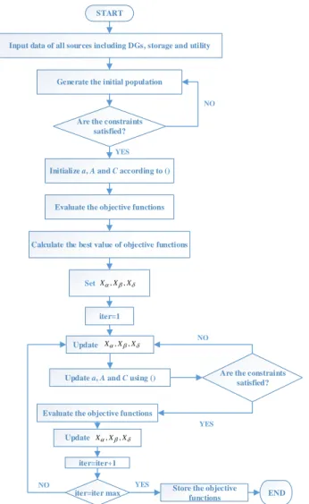
The flowchart of the proposed algorithm is illus-trated in Figure 1.
6.Simulation results
The effectiveness of the proposed MMOGWO al-gorithm is verified in this section where two cases are investigated. The MG of Figure 2 is considered as the test system. A 24-hour scheduling scheme is assumed for the analysis of the simulated system in order to clarify the performance of each power unit. Besides, the unity power factor is considered for all DGs, thus they just produce active power. The decision about power exchange between the MG and the utility, which is allowed at any hour in a day in order to more profitably exploit the market, is taken by MG central controller (MGCC). The data for the hourly active power of PV and WT, forecasted load demand and the utility power production bid, besides the en-tire bid data for all DGs along with the power market are available in [12]. PV and WT units do not con-sume any fuel at the times they produce electrical power during the day, consequently, the utility has to buy all electrical power produced by these units [12]. A Pareto-optimal set is attained for the two incom-patible objectives (cost and emission) in each case. It is worth mentioning that applying the proposed ap-proach for controlling the size of repository leads to the extraordinary fast convergence of the proposed MMOGWO that makes it superior among all other existing algorithms. The proposed method was im-plemented in MATLAB 8.1 and solved in a laptop with Core i5 CPU and 4GB RAM. The number of
population and maximum iteration are both consid-ered 100.
START
Input data of all sources including DGs, storage and utility
Generate the initial population
Are the constraints satisfied?
Initialize a, A and C according to ()
Evaluate the objective functions
Calculate the best value of objective functions
X X X , , Set iter=1 X X X , , Update
Update a, A and C using ()
NO
YES
Are the constraints satisfied? NO
Evaluate the objective functions
YES
Update X,X,X
iter=iter+1
iter=iter max NO
Store the objective functions YES
END
Fig. 1. Flowchart of the proposed algorithm. 6.1.First case
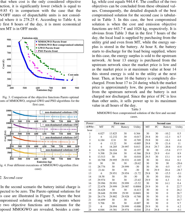
In this section, it is assumed that PV and WT (as non-dispatchable units) are in service at all hours during the day and are accepted to exploit at their maximum available output powers. This is while the ON\OFF states of dispatchable DGs (i.e. FC and MT) are considered. Therefore, in the algorithm process, the solutions for dispatchable units are compared with their minimum limit powers and if lower, the power will be put to zero. In this case no limits on the battery’s initial charge is considered. The Pareto op-timal front of this case is revealed in Figure 3, and results for three algorithms, including original
Fig 2. A typical MG test system [12].
GWO, PSO, and the proposed MMOGWO, are com-pared. The best compromised solution along with the values of the points where cost and emission are min-imum are depicted. It is observed that in solving the MOOM problem, in addition to fast convergence, the proposed MMOGWO algorithm is able to properly find the points where the objective functions are in their minimum values, and the Pareto optimal front maintains between these points, while one deficiency of the two other algorithms in dealing with the con-sidered MG energy management problem is the inca-pability to detect these points. Evidently, when the cost function is at its minimum value, 281.3 €, the emission is 862.8 kg. Besides, when emission de-creases to 455.9 kg, cost equals 857.2 €. The best compromised solution is calculated according to the procedure described in section 3.3 where the cost and emission objective functions are 373.4 € and 566 kg, respectively.
In order to justify the robustness and effective-ness of the proposed MMOGWO algorithm, the pro-gram is executed four times and results of these four different executions in the first case are revealed in Figure 4. Obviously, the achieved Pareto optimal sets in all four runs are approximately similar. It can be concluded that since the numbers of non-dominated
solutions saved in the repository in different runs of the program, which are 150, 150, 147 and 149 re-spectively for the first, second, third and fourth runs, are very close, the proposed algorithm is robust. Thereupon, not only can the proposed algorithm in-crease the convergence speed but also it dein-creases quiescence which results in getting away from local optimums. Consequently, the proposed MMOGWO proposes more robust and qualified solutions.
The power dispatch in the best compromised so-lution obtained using MMOGWO in this case is pre-sented in Tables 3 in details. From these results, it is concluded that all equality and inequality constraints are satisfied. In the dispatch of the battery, when the battery is charging the values of power are negative, while during the discharging hours the values of power are positive. However, for the utility the nega-tive values are representanega-tive of delivering energy to the upstream network, while the positive values are related to the times when energy is purchased from the upstream network. According to Table 3, since there is no limit on the battery charge, and the bid of the battery is less than other units, it sells power up to its maximum value in all hours of the day. Addition-ally, since the price of FC is less than MT, the pur-chased power from FC in different hours of the day is
more. The MT power is limited on its permissible minimum value in most of hours because of the high price of power in comparison with other units.
As is expected, it is evidently obvious from Table 4 that when cost is the only considered objective function, it is significantly lower (which is equal to 269.85 €) in comparison with the case that the ON/OFF states of dispatchable units is not consid-ered where it is 278.25 €. According to Table 4, in the first 8 hours of the day, it is more economical when MT is in OFF mode.
Fig. 3.Comparison of the objective functions Pareto optimal fronts of MMOGWO, original GWO and PSO algorithms for the
first case. 4500 500 550 600 650 700 750 800 850 500 1000 Emission (kg) non-dominated solutions=150 4500 500 550 600 650 700 750 800 850 500 1000 Emission (kg) non-dominated solutions=150 4500 500 550 600 650 700 750 800 850 500 1000 Emission (kg) C os t (€ ct) non-dominated solutions=147 4500 500 550 600 650 700 750 800 850 500 1000 Emission (kg) non-dominated solutions=149
Fig. 4. Four different executions of MMOGWO algorithm (first case).
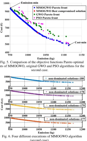
6.2.Second case
In the second scenario the battery initial charge is expected to be zero. The Pareto optimal solutions for this case are illustrated in Figure 5, where the best compromised solution along with the points where the two objective functions are minimum for the proposed MMOGWO are revealed, besides a
com-parison between three algorithms, original GWO, PSO, and MMOGWO, is performed. The minimum cost is equal to 484 €, while emission is 1114 kg; in Emission-minimum, the emission is reduced to 950.9 kg, while cost equals 944.4 €. The conflict of the two objectives can be concluded from these obtained val-ues. Consequently, the detailed dispatch of the best compromised solution for the second case is tabulat-ed in Table 3. In this case, the best compromistabulat-ed solution is when the cost and emission objective functions are 643.7 € and 1026 kg, respectively. It is obvious from Table 3 that in the first 7 hours of the day, the local load is supplied by purchasing from the utility grid and even from MT, while the energy sur-plus is stored in the battery. At hour 8, the battery starts to discharge for the load being supplied, where in this case, the energy surplus is sold to the upstream network. At hour 13 energy is purchased from the upstream network since the market price is low and as the market price is at maximum value at hour 14 this stored energy is sold to the utility at the next hour. Then, at hour 16 the battery is completely dis-charged. From hour 17 to 24 during which the market price is approximately low, the power is purchased from the upstream network and the battery is not charged nor discharged. Since the price of FC is less than other units, it sells power up to its maximum value in all hours of the day.
Table 3
MMOGWO best compromised solution of the first and second cases.
Power (kWh)
First case Second case
MT FC Battery Utility MT FC Battery Utility hour 1 6.027 13.825 30 0.364 30 30 -10.2 0.5 2 6 12.232 30 -0.017 29.8 30 -12.3 0.7 3 6.184 12.8 30 -0.769 29.8 30 -16.1 4.6 4 6 13.22 30 -0.005 29.8 30 -21.6 11 5 6 18.205 29.997 0.013 29.8 29.7 -20.8 15.6 6 6.258 26.024 30 -0.197 30 30 -15.6 17.7 7 9.398 29.184 30 -0.366 29.8 29.9 -0.4 8.9 8 13.513 30 30 -0.018 29.5 30 13.1 0.9 9 10.708 29.995 29.931 -0.169 30 30 10.4 0.1 10 30 30 30 -20.62 30 30 30 -20.6 11 28.776 30 29.999 -30 30 30 -0.5 -0.7 12 21.64 30 30 -30 30 29.9 20.4 -28.7 13 6 29.951 29.954 -21.72 29.8 30 -15.5 -0.1 14 18.58 30 30 -30 30 30 18.6 -30 15 29.974 30 30 -23.63 29.9 30 6.3 0.1 16 29.996 29.991 29.999 -15.52 30 30 14.1 0.4 17 22.678 29.999 29.987 0.0004 29.9 30 0 22.7 18 26.628 30 30 -0.413 30 30 0 26.2 19 28.648 29.999 29.99 0.0601 30 30 0 28.7 20 26.174 29.882 29.928 -0.768 30 30 0 25.2 21 16.699 30 30 0 30 30 0 16.7 22 9.706 30 30 -0.007 30 30 0 9.7 23 6 28.094 29.999 -0.008 29.9 30 0 4.2 24 6.046 19.381 29.974 -0.016 25.6 29.8 0 -0.1
Fig. 5.Comparison of the objective functions Pareto optimal fronts of MMOGWO, original GWO and PSO algorithms for the
second case. 9500 1000 1050 1100 1150 1200 500 1000 Emission (kg) 9500 1000 1050 1100 1150 1200 500 1000 Emission (kg) 9500 1000 1050 1100 1150 1200 500 1000 Emission (kg) C os t (€ ct) 9500 1000 1050 1100 1150 1200 500 1000 Emission (kg) non-dominated solutions=179 non-dominated solutions=180 non-dominated solutions=178 non-dominated solutions=177
Fig. 6. Four different executions of MMOGWO algorithm (second case).
Table 4
MMOGWO optimal solution achieved inthe firstcase where the cost is reduced to 269.85 €.
In Figure 6 a comparison between four executions of the algorithm in the second case is shown. Obvi-ously, the achieved Pareto optimal sets in all four runs are approximately similar. As is obvious from Figure 6, the numbers of non-dominated solutions saved in the repository in different runs of the pro-gram, which are 180, 178, 179 and 177 respectively for the first, second, third and fourth runs, are very close. Consequently, the robustness of the proposed
MMOGWO algorithm in the second case can be jus-tified through the results of Figure 6.
When the initial charge of the battery is zero, a strict restriction on the battery charge and discharge is put on. Consequently, the most adjustable scenario is when the battery has initial charge. Because of the more realistic performance of the battery in the sec-ond case, more power is purchased from MT, com-paratively. In both cases, in most hours a large amount of power is bought from FC since it is less expensive. In first hours of the day where the market price is lower, the system operator purchases power from the utility. This power can be utilized in order to supply local loads or can be stored in the storage device. However, in peak hours, the stored power can be sold to the utility in a much higher price.
The superiority of an optimization algorithm in solving multi-objective problems is concluded from the appropriate and fast convergence, while attaining exact Pareto front. Moreover, the robustness of an optimization algorithm can be another criterion in order to prove the effectiveness of the method. Con-sequently, as is concluded from the obtained results and by comparing the Pareto optimal sets of three algorithms in solving the MOOM problem, the pri-ority of the proposed MMOGWO algorithm along with its robustness and accuracy is justified. Accord-ingly, it is proved that the proposed MMOGWO has successfully fulfilled these assumed criteria, and it can significantly achieve the exceptional solution in comparison with other methods in solving MOOM problem of an MG.0
7.Conclusions
The new MMOGWO algorithm was proposed in order to deal with the multi-objective optimal opera-tion management in a typical MG. Three modifica-tions were added to the original GWO which result in more accurate and faster performance of the suggest-ed approach. The variable population size resultsuggest-ed from the first modification avoids trapping in local Power (kWh) MT FC Battery Utility hour 1 0 20.171 0.0445 30 2 0 17.924 0.2911 30 3 0 18.145 0.0699 30 4 0 19.129 0.1158 29.9706 5 0 24.159 0.0881 29.9679 6 0 29.906 2.1815 29.9976 7 0 29.992 8.3458 29.8773 8 0 30 18.6006 24.8944 9 29.991 29.999 30 -19.5251 10 30 30 30 -20.615 11 28.817 30 29.9576 -30 12 21.787 29.856 29.9964 -29.9997 13 14.186 29.999 30 -29.9992 14 18.729 29.855 29.9959 -29.9997 15 29.993 30 30 -23.6533 16 30 30 29.9995 -15.5295 17 30 30 30 -7.335 18 0 30 30 26.215 19 0 30 28.7922 29.9058 20 26.429 30 30 -1.2142 21 30 30 30 -13.3005 22 29.905 29.942 29.9868 -20.1343 23 0 30 4.085 30 24 0 25.188 0.2147 29.982
optima, while the two other modifications were aug-mented to the mutation procedure in order to increase the convergence speed and robustness of the algo-rithm. Additionally, a novel method was applied for controlling the size of repository which generates a well-distributed Pareto front in a very low computa-tional time. As a result, the accuracy and speed of the algorithm will improve. It is obvious from the results that an exceptional Pareto optimal set was achieved while applying the presented method comparing with original GWO and PSO algorithms. Two different scenarios were considered in order to justify the ef-fectiveness of MMOGWO. Simulation results mani-fest that the proposed method is able to deal with mixed-integer problems. Future works can include the following:
1. Investigating the stochastic MG optimal
oper-ation management while considering the un-certainties of renewable resources using the proposed algorithm.
2. Studying the effects of elements of the future smart grid, such as electric vehicles, in the considered MG energy management.
Acknowledgement
This work was supported in part by Royal Academy of Engineering Distinguished Visiting Fellowship under Grant DVF1617\6\45.
References
[1] M. Vosoogh, M. Kamyar, and A. Akbari, "A novel modifica-tion approach based on MTLBO algorithm for optimal man-agement of renewable micro-grids in power sys-tems." Journal of Intelligent & Fuzzy Systems vol. 27, (1), pp. 465-473, 2014.
[2] H. R. Baghaee, M. Mirsalim, and G. B. Gharehpetian, "Mul-ti-objective optimal power management and sizing of a relia-ble wind/PV microgrid with hydrogen energy storage using MOPSO," Journal of Intelligent & Fuzzy Systems vol. 32, (3), pp. 1753-1773, 2017.
[3] W. Gu, Z. Wu, R. Bo, W. Liu, G. Zhou, W. Chen, et al., "Modeling, planning and optimal energy management of combined cooling, heating and power microgrid: A review,"
International Journal of Electrical Power & Energy Systems,
vol. 54, pp. 26-37, 2014.
[4] N. Javidtash, M. Jabbari, T. Niknam, and M. Nafar, "A novel mixture of non-dominated sorting genetic algorithm and fuzzy method to multi-objective placement of distributed generations in Microgrids." Journal of Intelligent & Fuzzy Systems Preprint pp. 1-8, 2017.
[5] H. R. Kamankesh, and G. A. Vassilios, "A sufficient stochas-tic framework for optimal operation of micro-grids consider-ing high penetration of renewable energy sources and electric
vehicles." Journal of Intelligent & Fuzzy Systems vol. 32, (1), pp. 373-387, 2017.
[6] A. R. Abbasi, S. Abbasi, J. Ansari, and E. Rahmani, "Effect of plug-in electric vehicles demand on the renewable micro-grids," Journal of Intelligent & Fuzzy Systems vol. 29, (5), pp. 1957-1966, 2015.
[7] T. A. Nguyen, and M. L. Crow, "Stochastic optimization of renewable-based microgrid operation incorporating battery operating cost,"IEEE Transactions on Power Systems, vol. 31, pp. 2289-2296, 2016.
[8] K. W. Hu, and C. M. Liaw, "Incorporated operation control of DC microgrid and electric vehicle,"IEEE Transactions on Industrial Electronics, vol. 63, pp. 202-215, 2016.
[9] M. Marzband, E. Yousefnejad, A. Sumper, and J. L. Domínguez-García, "Real time experimental implementation of optimum energy management system in standalone mi-crogrid by using multi-layer ant colony optimization," Inter-national Journal of Electrical Power & Energy Systems, vol. 75, pp. 265-274, 2016.
[10] R. Jabbari-Sabet, S.-M. Moghaddas-Tafreshi, and S.-S. Mir-hoseini, "Microgrid operation and management using proba-bilistic reconfiguration and unit commitment," International Journal of Electrical Power & Energy Systems, vol. 75, pp. 328-336, 2016.
[11] M. H. Moradi, M. Abedini, and S. M. Hosseinian, "Optimal operation of autonomous microgrid using HS–GA," Interna-tional Journal of Electrical Power & Energy Systems, vol. 77, pp. 210-220, 2016.
[12] S. Parhoudeh, A. Baziar, A. Mazareie, and A. Kavousi-Fard, "A novel stochastic framework based on fuzzy cloud theory for modeling uncertainty in the micro-grids," International Journal of Electrical Power & Energy Systems, vol. 80, pp. 73-80, 2016.
[13] R. Cheng, T. Rodemann, M. Fischer, M. Olhofer, and Y. Jin, "Evolutionary Many-objective Optimization of Hybrid Elec-tric Vehicle Control: From General Optimization to Prefer-ence Articulation, "IEEE Transactions on Emerging Topics in Computational Intelligence, vol. 1, (2), pp. 97-111, 2017. [14] M. Zaman, S. M. Elsayed, T. Ray, and R. A. Sarker, "Evolu-tionary algorithms for dynamic economic dispatch prob-lems," IEEE Transactions on Power Systems, vol. 31, pp. 1486-1495, 2016.
[15] F. A. Mohamed and H. N. Koivo, "Multiobjective optimiza-tion using Mesh Adaptive Direct Search for power dispatch problem of microgrid," International Journal of Electrical Power & Energy Systems, vol. 42, pp. 728-735, 2012. [16] T. Lv, Q. Ai, and Y. Zhao, "A bi-level multi-objective
opti-mal operation of grid-connected microgrids," Electric Power Systems Research, vol. 131, pp. 60-70, 2016.
[17] A. Baziar and A. Kavousi-Fard, "Considering uncertainty in the optimal energy management of renewable micro-grids including storage devices," Renewable Energy, vol. 59, pp. 158-166, 2013.
[18] A. Kavousi-Fard, A. Abunasri, A. Zare, and R. Hoseinzadeh, "Impact of plug-in hybrid electric vehicles charging demand on the optimal energy management of renewable micro-grids," Energy, vol. 78, pp. 904-915, 2014.
[19] G. Aghajani, H. Shayanfar, and H. Shayeghi, "Presenting a multi-objective generation scheduling model for pricing de-mand response rate in micro-grid energy management," En-ergy Conversion and Management, vol. 106, pp. 308-321, 2015.
[20] S. Mirjalili, S. M. Mirjalili, and A. Lewis, "Grey wolf opti-mizer," Advances in Engineering Software, vol. 69, pp. 46-61, 2014.
[21] S. Rajasomashekar and P. Aravindhababu, "Biogeography based optimization technique for best compromise solution of economic emission dispatch," Swarm and Evolutionary Computation, vol. 7, pp. 47-57, 2012.
[22] S. Sharma, S. Bhattacharjee, and A. Bhattacharya, "Grey wolf optimisation for optimal sizing of battery energy storage device to minimise operation cost of microgrid," IET Gener-ation, Transmission & Distribution, vol. 10, pp. 625-637, 2016.
![Fig 2. A typical MG test system [12].](https://thumb-us.123doks.com/thumbv2/123dok_us/10949223.2983453/10.892.203.701.198.633/fig-a-typical-mg-test-system.webp)