Regional Convergence and Catch-up in India
between 1960 and 1992.
Kamakshya Trivedi
1 Nuffield College University of Oxfordemail: kamakshya.trivedi@nuffield.ox.ac.uk
December 2002. Comments Welcome. Abstract
This paper examines the evidence for regional convergence or catch-up in levels and growth rates of per capita income among the 16 major states in India between 1960 and 1992. The results — estimated using OLS, the within-group LSDV estimator, Re-Weighted Least Squares, and Least Trimmed Squares — establish that unconditional convergence in growth rates does not obtain, but that there is clear and robust evidence of conditional convergence. This suggests that important differences between observed state incomes are likely to be caused by different steady-state incomes, to which convergence occurs. The cross-state income distribution is analyzed and the greater polarization between states in terms of levels of income is established using measures of dispersion and kernel density estimates. A tentative conclusion is that a small group of states are pulling away from the rest of the distribution, causing an incipient second peak.
JEL Classification: O11, O40, O53 Keywords: India, Convergence, Growth
1This research was generously supported by Nuffield College, Oxford. I have benefited from the support
and advice of various people. I am most grateful of all to Gavin Cameron for constant encouragement and helpful supervision. Specific thanks are due to Chris Bowdler, Rui Fernandes, Adeel Malik, and Misa Tanaka for comments on an earlier draft. I would also like to thank seminar participants in the Development Workshop, Cambridge, and at the SMYE, Paris I-Sorbonne, for helpful feedback. Lastly, I am very grateful to Tim Besley, Robin Burgess, Rohini Pande, and the Economic Organization and Public Policy Programme, STICERD, LSE, for access to data; and Vijayan Punnathur and the Rai family for their hospitality and help in New Delhi. The standard disclaimer applies: responsibility for all remaining
1
Introduction
One of the key questions that the study of economic growth tries to answer is whether initially disparate regions of the world converge to common steady state paths. This issue ofconvergence orcatch-up — what it means or implies theoretically, and trying to find it within the data — has driven much of the resurgence in the study of economic growth at an aggregate level in the past decade and a half. This paper is part of that research: it is a comprehensive study of convergence in a panel of 16 states in India betweeen 1960 and 1992.
More specifically, this paper can also be considered a part of a growing agenda of ex-ploring the ideas of growth theory within low-income countries. Thefirst wave of empirical literature on growth was almost exclusively cross-country. Since then, as more data has become available, and as the limitations of cross-sectional and cross-country work have been better understood; more research has focussed on panel data and on within-country studies. In this respect, India is a rare and valuable example of a low-income country with long time series data for its constituent states. The data is by no means perfect.2 However, even with all the required caveats, comparability across states in India is likely to be better than the average cross-country study.
There are, thus, good academic reasons for learning about convergence within India. But currently there is also considerable interest in the social, political, and economic implications of convergence (or divergence) among the states. A recent Financial Times survey on India mentions that,
“India seems to be diverging into almost two different countries: prosperous socially stable, rapidly modernizing southern and western regions and poor and politically volatile northern and eastern regions”.3
What kind of income convergence is occurring, in actual fact, between the different states, would shed much light on such conjectures, and on other popular and academic debates about economic growth within India.4
It should be mentioned at the outset that while many implications of existing theories of economic growth and convergencefind empirical validation in the results reported here, none of the empirics were designed to explicitly test a particular theory versus another.
2
To give just one example, the state of Jammu and Kashmir has several missing observations for the conditioning variables used in section 3. It is thus omitted from the conditional convergence regressions. More details are provided in the relevant sections of the paper and in the data appendix.
3
Amy Kazmin, ‘The North-South Divide’, in theFinancial Times,November 19th, 1999.
4For instance, critics of India’s economic reforms programme launched in the 1990s have frequently
remarked that the reforms are responsible for the greater disparity in incomes between states. While this paper does not directly address this debate, the results in section 4 do establish that the growth of income disparity between states is not, by any means, a phenomenon that started in the 1990s.
While that is an important objective of empirical research, it is deliberately not the ob-jective of this paper. So for example, section 3 assesses the evidence onβ−convergence without attempting tofit the theoretical straightjacket of the Solow (1956) model.5 The main aim of this paper, to re-iterate, is on the issue ofconvergence orcatch-up — whether initially disparate states in India display any tendency in the data to converge to common steady state paths between 1960 and 1992. In addition, since the sample only comprises 16 states, a subsidiary aim is to assess the robustness of results by using alternative esti-mation procedures. Apart from documenting convergence or the lack thereof, the analysis will also enable us to identify some of the keyinfluential states which seem to be driving the empirical results.
The rest of this paper has the following structure. Section 2 clarifies the two main concepts of convergence which are prevalent in the literature and which are empirically examined in the paper, namelyβ and σ−convergence. The discussion is deliberately brief since the primary focus of this paper is the empirical evidence that follows. Sections 3 and 4 study the evidence on convergence, and comment on how thefindings are related with experiences of specific states. In particular, section 3 documents the absence of uncondi-tionalβ−convergence, but also strong and consistent evidence of conditional convergence. Section 4 is about σ−convergence. It analyses the cross-state income distribution using measures of dispersion and kernel density estimates, andfinds evidence of increasing cross-state income disparities, or σ−divergence. Section 4 also comments on how cross-state income inequality might or might not be related to individual income inequality. Finally, Section 5 concludes.
2
What kind of convergence?
Even as a large and burgeoning literature has investigated whether there exist forces that lead to convergence, there remains some disagreement about its exact definition. Barro and Sala-i-Martin (1995) identify two notions of convergence. First, there is the concept of
β−convergence, which also comes in twoflavours. Loosely, it can be understood in terms of the following question: do initially poorer states grow faster? More precisely, it is the idea that a poor economy tends to grow faster than a rich one, so that the poor region possibly tends to catch up with the rich one in terms of the level of per capita income. The most popular formal model underlying the idea that initially poorer regions might grow faster is the neoclassical growth model of Solow (1956).6 The key assumption that generates the convergence result in neoclassical models is diminishing returns to reproducible capital. The relatively less well off economy will have lower stocks of physical capital, and hence
5See Nosbusch (1999) for an attempt to test the Solow model using Indian data. 6
Note that models with technology diffusion or factor mobility would also implyβ−convergence. For a review of these models see chs. 3 and 8, Barro and Sala-i-Martin (1995).
higher marginal rates of return on capital. Therefore, for any given rate of investment, it will have faster growth in the transition phase. Note that suchβ−convergence implied by the Solow model is conditional; and perceptible only after other factors which may cause variation in steady states have been accounted for. Anything that drives apart investment rates in rich and poor regions will, ceteris paribus, drive their steady-state income levels apart, even as each region is converging to its diverging steady state.
In contrast to this, one can define a stronger kind of convergence that takes place unconditionally or absolutely, where initially poorer states grow faster, notwithstanding differences in initial conditions. In terms of the Solow (1956) model, if we postulate that all regions, in the long run, have no tendency to display variation in the rates of investment, capital depreciation, population growth, and so forth, then such a model would generate unconditional or absolute convergence to a common value of per-capita income.
The second concept of convergence, σ−convergence, concerns cross-sectional disper-sion. σ−convergence occurs if the dispersion of say, per capita incomes across regions declines over time. More generally, it focusses on the evolution of the cross-sectional in-come distribution — its shape and the movement of the distribution over time. Other things being equal, β−convergence may eventually lead to σ−convergence.7 However, if other things are not equal, perhaps because each region is subject to random disturbances, then
β−convergence need not imply a reduction in the dispersion of income levels. Hence, con-ditional β−convergence as implied by the Solow model, is consistent with σ−divergence. For instance, anything that drives apart steady-state incomes in rich and poor regions will lead toσ−divergence, although each region might still be (conditionally) converging to a diverging steady-state.
The following section in this paper evaluates the evidence on β−convergence. It sug-gests the absence of unconditional β− convergence, but strong and consistent evidence of conditionalβ−convergence once measures of human capital and physical infrastructure are controlled for. The reported speeds of conditional convergence are quite high, when compared to standard OLS estimates from cross-country studies. The overall implication is that there is no unconditional tendency for initially poorer states to grow faster.
Although the evidence in section 3 informs us about whether the poorer states are con-vergingon average, it tells us very little about whether these states have actually caught up or are falling further behind other states in terms of levels of per capita incomes. In a series of influential papers, Danny Quah has argued that the most fruitful way of thinking about the question of whether poor states are catching up with rich states over time, is to focus on the changing distribution of state incomes over time — in other words,σ−convergence.8 This is the subject of section 4. Analysis of the cross-state income distribution reveals no
7This is trivially true in the case of unconditional or absoluteβ
−convergence. In such a world history, in the sense of different initial conditions, does not matter.
8
evidence ofσ−convergence. In fact, there are many signs ofσ−divergence, and instances of catch-up are few and far between.
3
Estimating
β
−
Convergence: Conditional or Absolute?
3.1
Preliminaries
In their landmark paper, Mankiw, Romer, and Weil (1992) suggest that an augmented Solow model — which expresses growth as an explicit function of the determinants of the ultimate steady state and the initial level of income — is a ‘natural’ way to study conver-gence. If we run a regression which conditions for the determinants of steady states, like the investment rate in the Solow model, then we would expect a negative sign on the initial income coefficient. The idea is that within regions approaching the same steady state, the poorer ones will grow faster in thetransitional period. In essence, we follow this approach. However, since our aim is to evaluate the evidence ofβ−convergence in states within India, rather than to explicitly test a particular growth model that predicts convergence, we use a more general specification in the empirics that follow —a la Barro (1991) and Caselli, Esquival, and Lefort (1996). The typical cross-country study of economic growth is built on an equation nested in the following specification, which is consistent with the Mankiw
et al (1992) formulation as well,
ln(yi,t)−ln (yi,t−τ) =γln (yi,t−τ) +Σkj=1πjx
j
it−τ+µi+εit (1)
where,
yit is now real per capita income of countryiat time t.
xit are a set of conditioning variables, which capture differences in steady states
µi is the state specific fixed effect, which will pick up the influence of any omitted
variable that does not vary over time in a panel
εit is the transitory error term that varies across countries and time periods, and has
mean equal to zero
and, the coefficient γ identifies the convergence effect.
Equation (1) is consistent with a variety of neoclassical growth models that accept as a solution a log-linearization around the steady state of the form (see Barro and Sala-i-Martin, 1995),
lny(t)−lny(0) =−³1−e−λt´lny(0) +³1−e−λt´lny∗ (2) whereλis the rate of convergence.9
9Note that the relation betweenγandλis only approximate. This is because the growth rate is observed
as an average over an interval ofτ years rather than at a point in time. The implied instantaneous rate of convergenceλwill be slightly higher than the value indicated by the coefficientγ. λwill tend toγ asτ
The more general specification in equation (1) allows us to control for variables which might influence the steady-state level of income, but which are not included explicitly in Solow (1956). This approach is particularly useful, since state-level data on investment or capital — a key variable in the Solow model — is not available for most of the sample period. Instead, as described in section 3.3 we use proxies for physical and human capital in order to control for the different steady-state levels in most of the regressions.
3.2
Unconditional Convergence
Most evidence on unconditional convergence has come from within-country studies. Two well-known examples are US states (Barro and Sala-i-Martin, 1992) and Japanese Prefec-tures (Barro and Sala-i-Martin, 1995). In both cases the authorsfind evidence of uncon-ditional β−convergence over long sample periods — 100 years for US states and 60 years for Japanese prefectures — and also over much shorter subperiods within the same sample. More recently, de la Fuente (2002) records evidence of unconditionalβ−convergence across Spanish regions in each of the three decades between 1965 and 1995 — a time period very similar to this study. By contrast, empirical evidence on unconditional convergence from developing countries has been much less encouraging. In the two studies that I have seen — on Mexico (Juan-Ramon and Rivera-Batiz, 1996) and on China (Jian, Sachs, and Warner, 1996) — unconditional convergence is a much less robustfinding, and obtains only within limited time spans. Jian, Sachs, and Warner (1996) study the provinces of China between 1952 and 1993, andfind evidence of divergence in real per capita incomes except in period 1978-1990. Similarly, Juan-Ramon and Rivera-Batiz (1996), investigate Mexico’s states in the 23 year period from 1970 to 1993, and report convergence in incomes between 1970-85 and divergence thereafter.
Moving to India, two papers have focussed on the issue of convergence among states in India between 1960 and 1992. Cashin and Sahay (1996) use a cross-section regression and report evidence of unconditionalβ−convergence, although the convergence rate that they estimate is not statistically significant. They further sub-divide the 30 year period into three 10 year long time-spans, andfind the strongest evidence of unconditional con-vergence in the decade 1961-71. On the other hand, even after controlling for shocks to the agricultural and manufacturing sector theyfind a conditional convergence rate of 1.5% per year, which is surprisingly low — lower even than the 2% reported from cross-country work. Their sample considers 20 states: the 16 major states considered in this paper plus 3 smaller states (Himachal Pradesh, Manipur, and Tripura), and the then Union Territory of Delhi. Bajpai and Sachs (1996) consider the same sample excluding Himachal Pradesh, and they also report evidence of statistically significant unconditional convergence in the decade of the 1960s, but not thereafter.10 They suggest that this could be the result of
In co m e G row th , 1960-70
MA Ln real state PerCapita income, 1960
gro Fitted values
6.4 6.6 6.8 7 7.2 -.05 0 .05 1 2 3 4 7 8 9 10 11 14 15 16 18 20 21 In co m e G row th , 1970-80
MA Ln real state PerCapita income, 1970
gro Fitted values
6 6.5 7 7.5 -.04 -.02 0 .02 .04 1 2 3 4 5 7 8 9 10 11 14 15 16 18 20 21 In co m e G row th , 1980-90
MA Ln real state PerCapita income, 1980
gro Fitted values
6.5 7 7.5 -.02 0 .02 .04 .06 1 2 3 4 5 7 8 9 10 11 14 15 16 18 20 21 In co m e G row th , 1965-92
MA Ln real state PerCapita income, 1965
ingr6592 Fitted values
6.2 6.4 6.6 6.8 7 .01 .02 .03 1 2 3 4 5 7 8 9 10 11 14 15 16 18 20 21
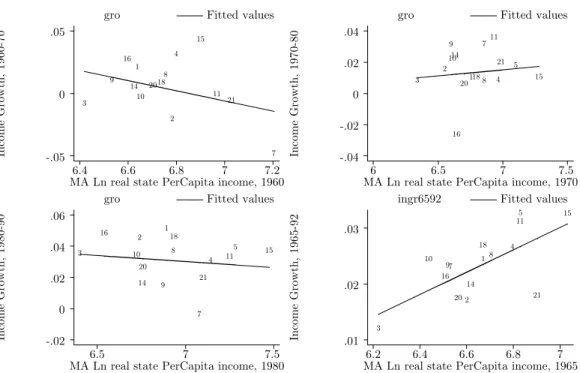
Figure 1: UNCONDITIONAL CONVERGENCE, 1960-92
high growth in the agricultural sector in India during the 60s.
There are a number of econometric concerns with both these studies. Most crucially, since their cross-sectional regression results are based on very few observations, sensitivity to outliers is likely to be a major problem. In fact, this possibility is never considered in either of the papers; and indeed, the econometric results of both papers often appear to be driven substantially by a few outlying states such as Delhi and Manipur.11 In small sample cross-section or panel econometrics, it is especially important to ensure that a few influential but atypical observations don’t distort parameter estimates, and that the results reflect trends in the majority of the sample. Temple (2000) suggests using robust estimation procedures alongside OLS estimates. A large difference between the results is a warning that conclusions drawn from standard estimating techniques such as OLS are being driven by a minority of observations. This estimation strategy is followed in the convergence regressions reported below.
of 99%.
1 1
This is particularly problematic since Delhi and Manipur are very tiny states. Together both these states account for less than 1.5% of India’s population, and approximately 2.5% of India’s GDP. Delhi is really a city — it has been granted statehood only in the 90s. It has the highest per capita income — hardly surprisingly since it is the capital city; and one of the lowest growth rates during the period. Manipur, on the other hand, is a poor and economically backward state in the Northeast, and has had a high growth rate up until the 90s.
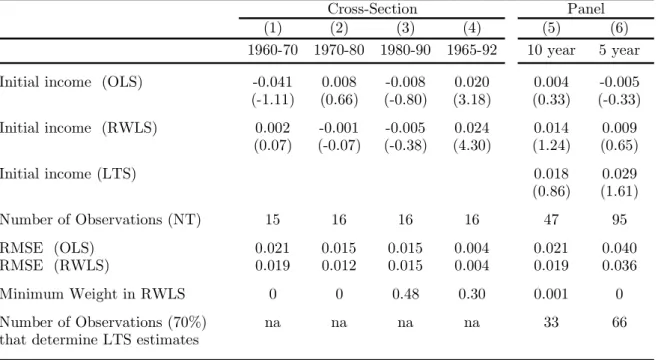
Thefirst part of table I reports the cross-sectional regression estimates. Since both the papers cited above — Cashin and Sahay (1996) and Bajpai and Sachs (1996) — use 10 year spans, columns (1), (2) and (3) report regressions for the three decades 1960-70, 1970-80 and 1980-90. The estimated model is of the following form:
growthi,1960−70=constant+γ(income)i,1960+εi (3)
and so on for another two points in time: 1970-80 and 1980-90.12 In terms of equation (1), ∆yit is growth over a 10 year interval, andyit−1 is in fact the level of income lagged 10 years, and so on. The 10 year interval should clean out the growth rate from any short termfluctuations such as business cycles, a pre-election year spending boom, or simply a bad monsoon. It is equally important to control for measurement error and business cycle variation in the right-hand side variables, so in fact, we use a 3 period moving average of lagged income.13 Note that equation (3), as written out, does not control for any determinants of steady state, and so a negative and significant value of γ would imply unconditional or absolute convergence to a common steady state.
Column (1) for the decade 1960-70 has only 15 observations since income data on Haryana is not available until 1965. The OLS coefficient on initial income is negative, sug-gesting unconditional convergence, but it is not statistically significant. The corresponding regression line is shown in panel 1 offigure 1. There appears no obvious negative relation between growth and initial income, but Jammu and Kashmir (state==7) looks like an outlier which might be influencing the regression estimate. To investigate this possiblility more formally, we compute a Re-Weighted Least Squares (RWLS) estimate, which is less sensitive to outliers than standard OLS.14We begin by estimating an OLS regression, and calculating Cook’s distance, D — where Di is a scaled measure of the distance between
the coefficient estimates when theith observation is omitted and when it is not.15 Next, any gross outliers for whichD >1 are eliminated. After this initial screening a series of weighted regressions are performed iteratively. Iterations stop when the maximum change in weights drops below a certain predetermined level of tolerance. Weights derive from two weight functions used successively —Huber weights and biweights — wherein cases with larger residuals receive gradually smaller weights. The RWLS estimate of initial income
1 2
The time periods over which growth rates are measured is varied in the exercises below; but for the sake of consistency, unless otherwise mentioned, all growth rates refer to average annual real per capita income growth rates over the period.
1 3However, using only the initial period income value — which is what most convergence studies do —
makes no qualitative difference to the result.
1 4
The RWLS estimate is computed using the RREGcommand in STATA 7.
1 5Cook’s Distance, D,can be thought of as an index which is affected by the size of residuals — outliers
— and the size of the leverage of each observation. Large residuals raise the value of D, as does high leverage. For the exact formulae, relation with other outlier diagnostics, and additional references see the Stata Reference Manual, Release 7.
is positive in contrast to the OLS estimate, suggesting that faint signs of unconditional convergence from the OLS estimates were in fact,red herrings. Given their small samples, similar problems with outliers and leverage points could well have plagued thefindings of unconditional convergence cited above.16
Column (2) reports the unconditional convergence estimates for 1970-80. The OLS estimate on initial income is positive and insignificant. Panel 2 infigure 1 suggests that there is no discernible pattern amongst the states in this period. The RWLS estimate confirms this — the coefficient estimate is negative, but it is not statistically different from zero. Column (3) spans the decade 1980-90. Both the OLS and the RWLS estimates are negative, but in both cases they are estimated extremely imprecisely, and we cannot reject a t-test that the coefficients are in fact zero. Thus, there is no convincing evidence of unconditional convergence in any of the three decades between 1960 and 1990.
In column (4) we estimate the model for the entire period between 1965 and 1992. The OLS estimate is positive and statistically significant, suggesting unconditional divergence. Panel 4 offigure 1 shows the corresponding regression line. Atfirst glance the relationship does not seem to be driven by outliers. The RWLS estimate confirms this. The positive coefficient is slightly bigger and estimated more precisely when the apparent outlier state, West Bengal (state==21) is downweighed. In fact West Bengal (state==21) appears to be one of the few “unconditionally convergent” states, as seen in panel 4 offigure 1. In 1965 it is one of the richest states in the sample, but over the 30 year period it has one of the lowest growth rates. On the other hand, the main examples of divergent states appear to be Punjab (state==15) at the top end, and Bihar (state==3) at the bottom end. Punjab (state==15) was the richest state in the 1960s, and has maintained one of the highest growth rates over the 30 year period on the back of strong agricultural performance. By contrast, Bihar (state==3) was the poorest state in the sample in the 1960s and it has barely grown over the 30 year period.
In columns (5) and (6) of table I, the panel versions of the unconditional convergence regressions specified in equation (3) are estimated. In column (5) we start with a 10 year panel, but following Islam (1995), we also rerun the regressions at 5 year intervals in column (6), to check if this makes any difference. The OLS estimate of initial income in the 10 year panel is positive but insignificant. The RWLS estimate is positive and more precisely estimated, but is still a long way away from statistical significance. For the 5 year panel in column (6), the OLS estimate is negative, but again estimated too imprecisely to be taken seriously. The RWLS estimate is positive, and estimated somewhat more precisely, but is nevertheless statistically insignificant.
The panel estimates afford a larger number of observations than the cross-sectional
1 6Looking closely at the weights from RWLS reveals that Jammu and Kashmir (state==7) is
regressions. This allows us to use the Least Trimmed Squares (LTS) estimator, due to Rousseeuw and Leroy (1987), to check if there is any negative relationship between growth and initial income in the majority of the data, rather than in the entire sample. LTS minimizes the sum of squares over a fraction — say 70% — of the observations, the chosen fraction being the combination which gives the smallest residual sum of squares. Temple (2000) points out that LTS estimators are “particularly well suited to an exercise such as a growth regression, where the idea is to learn about possible generalizations in the context of many disparate countries, some of which may be exceptions to the general pattern.” The LTS estimator can be thought of as a robustness check as well. Since diagnostics like Cook’s distance (used in RWLS) evaluate each observation separately, they might not be sufficient if pairs or groups of outliers exert undue influence but mask the influence of each other when testing for a single one. The LTS estimator is therefore particularly useful in the presence of multiple outliers or leverage points.
There are, however, drawbacks in throwing away 30% of one’s sample. It is possible that LTS would omit ‘good’ leverage points — those which affect the precision of the estimated coefficients rather than the point estimates. Note that standard errors for the LTS estimates are obtained by bootstrapping the data, and should be interpreted accordingly. In addition, Temple (2000) mentions that in confining oneself to a part of the data which the model describes well, there is a danger that even a poor model would fit relatively well in the restricted sample. Keeping these drawbacks in mind, we will focus primarily on the sign of LTS point estimates, as a supplementary check on the results from the other estimation methods.
The LTS estimates of initial income are reported in columns (5) and (6). In both cases they are positive, and in terms of magnitude, they are similar to the cross-sectional estimates for the entire period in column (4). This is evidence that the majority of the data exhibit no trend towards unconditionalβ−convergence.
To sum up: the regression estimates provide no evidence of absolute β−convergence amongst the major Indian states between 1960 and 1992, regardless of the length of time-span examined. If anything there is slight evidence of absoluteβ−divergence, albeit based on a small sample of 16 states.17 This conclusion is robust and contradicts previous work on unconditional convergence across Indian states cited above. A more tentative conclusion also seems to emerge from this evidence: unconditional convergence for regions within low-income countries — China (Jianet al,1996), Mexico (Juan-Ramon and Rivera-Batiz, 1996), and this study — seems at best, non-robust, and at worst, non-existent. This
1 7In Trivedi (2000), I have also checked for unconditional convergence in an expanded sample of 24
states based on an alternative dataset which contains comparable incomes data between 1980 and 1995. This sample includes the 4 of the smaller North-Eastern states, Himachal Pradesh, and the former Union Territories of Delhi, Goa, and Pondicherry. For the sake of brevity the results are not reported here, but even in this expanded sample there is no evidence of absoluteβ−convergence.
is unlike the case of US states (Barro and Sala-i-Martin, 1992), Japanese prefectures, or European regions, (Barro and Sala-i-Martin, 1995), or indeed regions withing Spain (de la Fuente, 2002), for which there is clear evidence of unconditional convergence.18 However, this should not be pushed too far, because the studies on the US, Japan, and Europe, (but not Spain), use longer spans of data than the studies on Mexico, China, and this current work on India.
(1) (2) (3) (4) (5) (6)
1960-70 1970-80 1980-90 1965-92 10 year 5 year Initial income (OLS) -0.041 0.008 -0.008 0.020 0.004 -0.005 (-1.11) (0.66) (-0.80) (3.18) (0.33) (-0.33) Initial income (RWLS) 0.002 -0.001 -0.005 0.024 0.014 0.009 (0.07) (-0.07) (-0.38) (4.30) (1.24) (0.65) Initial income (LTS) 0.018 0.029 (0.86) (1.61) Number of Observations (NT) 15 16 16 16 47 95 RMSE (OLS) 0.021 0.015 0.015 0.004 0.021 0.040 RMSE (RWLS) 0.019 0.012 0.015 0.004 0.019 0.036 Minimum Weight in RWLS 0 0 0.48 0.30 0.001 0 Number of Observations (70%) na na na na 33 66
that determine LTS estimates
TABLE I: UNCONDITIONAL CONVERGENCE (1960-90)
Notes: t-statistics are reported in parentheses. For OLS estimates, t-statistics are computed using heteroscedasticity corrected (Huber/White/Sandwich) estimates of standard errors. For LTS estimates, RMSE is the Root Mean Square Error. Constants not reported.
Cross-Section Panel
Dependent Variable: Growth Rate of Real State PerCapita Income
t-statisics are based on Bootstrapped standard errors (using 1000 replications).
3.3
Conditional Convergence
Much cross-country work has documented the presence of conditional convergence, i.e. poorer countries growing faster only after variables that determine the steady state level of output have been controlled for. Based on early cross-sectional work a convergence rate of 2% was given much credence (Barro and Sala-i-Martin, 1995). Later panel data studies
1 8One explanation for this could be that greater diversity in economic, social and political characteristics
and institutions obtains within regions of large developing countries such as Indian states, in comparison to developed countries. The assumptions that generate unconditional convergence in models like Solow (1956) — such as similar preferences and technologies, as well as basic institutions — are more likely to be true in more developed countries.
have reported convergence rates well in excess of 10%.19 In the Indian context Nosbusch (1999) and Nagaraj, Varoudakis and Veganzones (1998) report evidence of conditional convergence across states. Nosbusch (1999) is an attempt at fitting the textbook Solow model to state-level data in India, with the savings rate, population growth, and depre-ciation as the right-hand side variables. It reports high rates of conditional convergence — ranging from 7% in a regression without human capital, to 36% in a regression with human capital. Nagarajet al (1998) study the period betwen 1970 and 1994 andfind sys-tematic evidence of conditional convergence, with rates varying from 18% to 48%. Their study emphasizes inter-state differences in various types of social, economic and physical infrastructure, and on whether these can explain differences in inter-state growth rates.20 Testing for conditional convergence involves introducing variables which might deter-mine the steady state to the right hand side of the previous regressions. What variables a particular researcher chooses to include in the vector x depends on economic theory,
a priori beliefs about the growth process, and data availability. The data availability constraint is especially binding when working on a panel of states within a low income developing country. Missing values occur quite often, in particular, in the case of Jammu and Kashmir. Hence in the conditional convergence regressions reported in table 2, the state of Jammu and Kashmir is dropped from the sample under estimation.
Since the aim of this paper is to look for forces of convergence in the data, and not to test a particular model of convergence, a good place to start thinking about the condition-ing variables is a robustness study. In the baseline specification used to test robustness of the many different variables found in the empirical growth literature, Levine and Renelt (1992) choose the initial level of income, the investment rate, the secondary school enroll-ment rate, and the rate of population growth. In his study, Sala-i-Martin (1997) chooses the initial level of income, life expectancy and primary school enrollment rate at the start of the period. Life expectancy is used to proxy for non-educational human capital, while school enrollment is used to proxy educational human capital. Initial income captures the conditional convergence effect. According to Sala-i-Martin (1997), these variables have certain properties that make them the appropriate benchmark to test against: “...they have to be widely used in the literature, they have to be...evaluated at the beginning of the period...to avoid endogeneity, and they have to be...somewhat ‘robust’ in the sense that they systematically seem to matter in all regressions run in the previous literature.”
Following from this, we use the infant mortality rate and the high school school en-rollment rate to proxy for non-educational and educational human capital.21 The other
1 9
For example, Caselli, Esquival, and Lefort (1996).
2 0A key difference between Nagarajet al (1998) on the one hand, and Nosbusch (1999) and this paper
on the other, is in our use of price deflators which vary across states as well as over time. This is important in view of the subcontinental dimensions of India.
obvious variable to include in order to control for study of steady-state incomes is physical capital. Unfortunately, there is no good capital formation data available at the state-level in India, until very recently. Hence, we use a principal components measure of physical in-frastructure based on two series on energy production (installed capacity and generation), one series on energy consumption (high voltage electricity consumption by industry), and one series on the length of state highways.22 More details on the sources and construction of all these variables can be found in the data appendix.
A methodological concern which needs to be addressed at this stage relates to the pos-sible endogeneity (or reverse causality) of the right-hand side variables in the conditional convergence regressions. Simultaneity is pervasive given the nature of most of the regres-sors utilized. For example, it is not a priori obvious whether school enrollment affects growth by increasing human capital in an economy, or if economic growth affects school enrollment by improving schooling resources. This may happen because better economic growth increases the amount of resources that can potentially be diverted to schooling.23 Instrumental Variable estimation is an option if good instruments are available. In prac-tise, however, it is notoriously difficult to find variables that are both highly correlated with the endogenous variables, and which could plausibly have been left out of the regres-sion on growth in the first place. One solution lies within the panel set-up of the data, and involves using lags of the right-hand side variables, so that they are pre-determined with respect to the dependant variable. Many of the variables employed as determinants of either growth or the steady state income level, are likely to have their effect after a lag anyway. Given the dimensions of the panel and its reduced form, it seems sensible to use 5 year lags of the control variables. In the estimates reported below, an average of the value of the variable over the previous 5 years is computed and used as a regressor. This avoids randomness in the value of a given variable in any one of the previous 5 years from overwhelmingly influencing the estimated coefficients, and retains valuable information contained in the annual data.24 So for a panel based on equation (1) for example, thefirst brief, apart from census based literacy rates, which are measured across 10 year intervals, the high school enrollment is one of the most reliable measures of education available annually at the state level. The infant mortality rate is used because estimates of the commonly used measure — life expectancy at birth — are not available for states in India until after the 1970s.
2 2The statistical technique of Principal Components analysis is fairly standard, and explained in
Dunte-man (1989). It enables the combination of an original set of variables into a single variable which represents most of the variation in the original set.
2 3Note however, that this does not appear to be the case with Indian states. Richer states do not always
spend more on education and social services in per capita terms than poorer states.
2 4
It might be argued that even 5 years is too short a time span to fully partial out the effect of short term cycles and shocks. However, longer intervals will reduceT and therefore accentuate the familiar ‘Nickell (1981) bias’ in dynamic panel data models with fixed effects. In an ideal world, (T → ∞), I believe, between 10 and 20 years might be an appropriate span.
two cross-sections in time withfixed effects will look like,
growthi,1960−65 = γ(income)i,1965+Σkj=1πjxji,1955−60+µi+εit (4)
growthi,1965−70 = γ(income)i,1965+Σkj=1πjxji,1960−65+µi+εit (5)
and so on. Such a specification rules out contemporaneous correlation between the right-hand side variables and the error term.
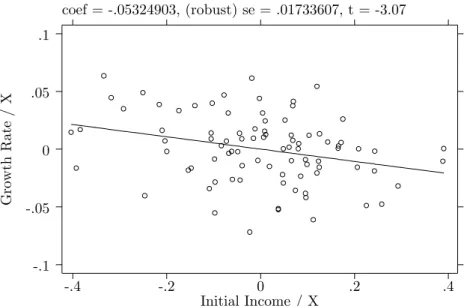
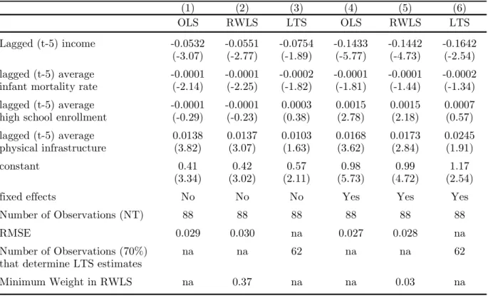
Column (1) of table II reports the OLS estimates of a regression of growth on initial income and the three control variables without the fixed effects, µi. The key result is that lagged income is now negative and statistically significant — evidence of conditional convergence. The speed of the convergence is approximately 5.3% a year. At this rate, it would take a state close to 13 years to get half way towards its steady state output.25 Figure 2 shows the partial relation between growth and initial level of income, as implied by the regression in column (1).26 In contrast to the lack of a clear pattern between growth and initial income infigure 1, it clearly depicts the conditional convergence effect. The graph also seems to indicate that the relation is not being driven by a few outliers. More rigorous confirmation of this fact is provided by the robust estimation procedures in columns (2) and (3) in the same table.
Of the other conditioning variables, the infant mortality rate has a statistically sig-nificant negative effect and physical infrastructure has a statistically significant positive effect on the steady state level, and hence on transitional growth. The education variable has a negative coefficient, but it is too poorly estimated to be taken seriously.
Column (2) provides the RWLS estimates of the same regression. There is very little difference in the OLS and RWLS coefficient estimates, and the standard errors are also roughly the same. The LTS estimates in column (3) are more instructive. They also confirm the presence of conditional convergence — in fact the bigger value of the coefficient on initial income suggests that when attention is restricted to the chosen 70% of the sample, the tendency towards conditional convergence is even more clearly apparent. However, the notable change from columns (1) and (2) is that the LTS estimate of high school enrollment is positive (but still estimated very imprecisely). Closer inspection of the
2 5
This can be calculated by noting that the half-life, sayt∗, of a variable growing at a constant negative growth rate (in this caseλ), is the solution toe−λt∗= 0.5. Taking logs, t∗' 0.λ69. Recall from equation (2) that in the vicinity of a balanced growth path,lny(t)−lny∗evolves as
lny(t)−lny∗=e−λt[lny(0)−lny∗]
2 6The vertical axis on the graph plots the residual growth rate after filtering out the parts explained
by all the explanatory variables other than initial income. The horizontal axis plots the corresponding residual element of initial income. Thefitted line is from an OLS regression, and has the same slope and standard error (up to a degree of freedom adjustment) as the estimated coefficient and standard error from the regression in column (1) of table II.
coef = -.05324903, (robust) se = .01733607, t = -3.07 G rowth R a te / X Initial Income / X -.4 -.2 0 .2 .4 -.1 -.05 0 .05 .1
Figure 2: GROWTH RATE VERSUS INITIAL INCOME: PARTIAL RELATION FROM COLUMN (1), TABLE II
residuals from the LTS estimates reveals that all observations from Kerala (state==9) except one, had the highest residuals. Kerala is an atypical state, with exceptionally high levels of education, but with only an average level of income.27 Re-estimating the OLS regression in column (1) without Kerala produces a positive and significant coefficient on high school enrollment (estimate=0.001, t-statistic=2.17), and leaves the sign and significance of the other estimates unchanged.28
Table II column (4) adds fixed effects to the previous specification. In the growth lit-erature Islam (1995) was thefirst paper to clarify the use of thefixed effect in panel data estimation. It will capture the influence of any omitted variable that causes persistent differences in state-specific production functions. It can thus be thought of as controlling for initial conditions — resource endowments, climate, institutions and so forth. In prin-ciple, one could use Instrumental Variable estimation, but given the nature and scope of initial conditions and given that so many variables can be thought of as affecting economic growth, suitable instruments are unlikely to be easy to come by. Temple (1999) explains that the chief alternative is to use afixed effects panel data specification:
2 7Between 1960 and 1992, Kerala had an average high school enrollment rate of 80.8% against an average
of 41.3% for the entire sample. For the same period, its real per capita income was marginally below the sample average. For a more detailed analysis of Kerala’s unique developmental achievements, see Drèze and Sen (1995).
2 8It is interesting — but not entirely unexpected — that since all Kerala observations were, in a sense,
‘outliers’ or ‘influential’, RWLS estimates, which evaluate each observation separately, were unable to correct for this.
“In the absence of a suitable proxy..., the only way to obtain consistent es-timates of a conditional convergence regression is to use panel data methods. Since initial efficiency is an omitted variable that is constant over time, it can be treated as a fixed effect, and the time dimension of a panel used to eliminate its influence.”
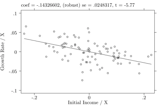
Controlling for state-specific initial conditions raises the speed of convergence quite substantially in column (4). The negative coefficient on initial income goes up by a factor of three (compared to the corresponding OLS estimate without fixed effects in column (1)), and it is very significant. This increase is in line with previously reported results in the panel data literature — both cross-country and from India.29 The coefficient on infant mortality is unchanged but is statistically significant only at the 10% level. On the other hand, the coefficients on physical infrastructure and high school enrollment increase in value, and they are both statistically significant. Figure 3 depicts the relation between growth and initial income from column (4), constructed analogously tofigure 2. The bigger conditional convergence effect is apparent, and it does not seem to be driven by influential outliers. Thefixed effects are not reported separately, but they are collectively significant. An F-test that all the fixed effects are equal to zero is rejected with a p-value of 0.003. This suggests that the process ofβ−convergence is impeded by persistent differences in initial conditions across states.
Columns (5) and (6) provide the robust regression estimates for the conditional con-vergence regression with fixed effects. Once again, the RWLS coefficient estimates are very similar to the OLS estimates, except that the standard error for the coefficient on the infant mortality rate is bigger. The LTS estimates emphasize the conditional convergence effect and the impact of physical infrastructure relative to the OLS and RWLS estimates.30 Overall, conditionalβ−convergence is a robust characteristic of per capita income across states in India between 1960 and 1992.
To summarize this section, we have examined the twin hypotheses of conditional and unconditionalβ−convergence whichflow from Neoclassical growth models like Solow (1956). By so doing, we have in large part answered an extememly important question about whether poorer states in India grow faster, on average. The empirical results pre-sented here suggest that unconditional β−convergence does not obtain, and that this is a robust feature of the data. This reverses the findings and implications of some of the previous studies on regional convergence in India cited above. On the other hand, there is strong and consistent evidence of convergence once factors that affect steady-state levels
2 9
See Islam (1995), Caselliet al (1996), and Nagarajet al (1998) among others.
3 0Note that the bootstrapped standard errors calculated for the LTS estimates in column (6), table II,
are much less reliable than those calculated elsewhere in tables I and II. This is because the bootstrapping algorithm in S-Plus encounters singularity problems on account of the fixed effects in this particular specification. Nevertheless, the resultantt-statistics are reported for the sake of consistency.
coef = -.14326602, (robust) se = .0248317, t = -5.77 Growth R a te / X Initial Income / X -.2 0 .2 -.1 -.05 0 .05 .1
Figure 3: GROWTH RATE VERSUS INITIAL INCOME: PARTIAL RELATION FROM COLUMN (4), TABLE II
of income are controlled for. These include proxies for educational and non-educational human capital, physical capital, and initial conditions. Poorer states do indeed grow faster than richer states in their transition phases, but they are growing towards differing steady states. Another key result is the high rates of conditional convergence — between 5 and 15 percent with different specifications.31 This implies that the average time an economy spends to cover half of the distance between its initial position and its steady state ranges from 5 to 15 years. Given these relatively high speeds of convergence, many economies will usually be close to their steady states, and important differences in per capita income levels across states will mainly be explained by differences in their steady state values. Consequently, studying movements of income levels becomes especially significant to un-derstand whether states are, in fact, catching up with each other or falling behind. In other words, one needs to understand how the cross-state income distribution is evolving over time.
3 1These estimates lie at the lower end of the range of estimates for conditionalβ
−convergence recorded in previous work on India. In related work, Trivedi (2000) has reported higher rates of convergence — up to 25% — with a bigger set of variables controlling for steady-state levels.
(1) (2) (3) (4) (5) (6)
OLS RWLS LTS OLS RWLS LTS
Lagged (t-5) income -0.0532 -0.0551 -0.0754 -0.1433 -0.1442 -0.1642 (-3.07) (-2.77) (-1.89) (-5.77) (-4.73) (-2.54) lagged (t-5) average -0.0001 -0.0001 -0.0002 -0.0001 -0.0001 -0.0002 infant mortality rate (-2.14) (-2.25) (-1.82) (-1.81) (-1.44) (-1.34) lagged (t-5) average -0.0001 -0.0001 0.0003 0.0015 0.0015 0.0007 high school enrollment (-0.29) (-0.23) (0.38) (2.78) (2.18) (0.57) lagged (t-5) average 0.0138 0.0137 0.0103 0.0168 0.0173 0.0245 physical infrastructure (3.82) (3.07) (1.63) (3.62) (2.84) (1.91)
constant 0.41 0.42 0.57 0.98 0.99 1.17
(3.34) (3.02) (2.11) (5.73) (4.72) (2.54)
fixed effects No No No Yes Yes Yes
Number of Observations (NT) 88 88 88 88 88 88
RMSE 0.029 0.030 na 0.027 0.028 na
Number of Observations (70%) na na 62 na na 62
that determine LTS estimates
Minimum Weight in RWLS na 0.37 na na 0.03 na
Notes: t-statistics are reported in parentheses. For OLS estimates, t-statistics are computed using heteroscedasticity corrected (Huber/White/Sandwich) estimates of standard errors. For LTS estimates, RMSE is the Root Mean Square Error.
TABLE II: CONDITIONAL CONVERGENCE Dependent Variable: Growth Rate of Real State PerCapita Income
t-statistics are based on Bootstrapped standard errors (using 1000 replications).
4
Looking for
σ
−
Convergence
4.1
Preliminaries
As noted above, conditional β−convergence does not necessarily imply that states are actually coming closer together in terms of levels of income. In fact, even if we had found unconditionalβ−convergence between states in India, this would imply convergence in lev-els of income only in the complete absence of any random shocks which might push states away from each other. Hence, a sensible way of thinking about the question of whether poor states are catching up with rich states over time, is to focus on the changing distri-bution of state incomes over time. This is the idea behind the notion ofσ−convergence. So, in this chapter we examine the issue of catch-up and convergence by directly studying the cross-state distribution of levels of income.32 In section 4.2, we start by examining
3 2The term ‘distribution’ is used somewhat loosely here, and in what follows. With only 16 points at any
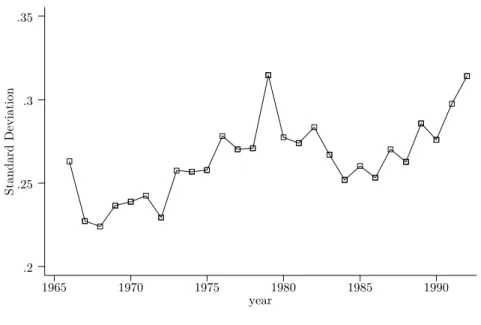
St andar d D evi at io n year 1965 1970 1975 1980 1985 1990 .2 .25 .3 .35
Figure 4: STANDARD DEVIATION OF THE CROSS-STATE INCOME DISTRIBUTION, 1965-92
the dispersion of the cross-state income distribution over time. This gives us the first clear evidence ofσ−divergence in the data. Evidence from kernel density estimates is also presented; and it is shown that in fact, the cross-state income distribution is characterized by persistence, catching-up, and falling behind, all at once, even as the distribution as a whole spreads out over time. In section 4.3, an important qualifications to these findings of increased income disparity is provided. By weighing state incomes by their respective populations, it is shown that an upward trend in individual income inequality is most clearly evident only after the mid-1980s.
4.2
How is the Cross-State Income Distribution Evolving over Time?
A straightforward way to check forσ−convergence is to look at the standard deviation of the cross-state income distribution over time. Figure 4 plots the standard deviations from 1965 to 1992 of the log of real state per capita incomes across all the 16 states. Apart from a brief period in the late 1960s and in thefirst half of the 1980s, there is a discernible increase in the cross-state income dispersion, which looks set to continue into the 1990s. This is a sign of σ−divergence. However, from figure 4 it is not clear what states are driving this increase in dispersion — are these states at the core or the periphery of the cross-state distribution?
however, studying the cross-state income spread yields some interesting and consistent insights even for this small sample.
Figure 5 depicts a series of Tukey Box Plots for the sample of 16 states.33 In con-structing these box plots a normalized measure of income is used in order to facilitate comparison.34 The figure shows that the upper and lower adjacent values in 1991 are much further apart relative to say, 1966, indicating the increased disparity between the richest and poorest states. The key insight from thisfigure is that the inter-quartile range (the middle 50% of the cross-state distribution) has only moderately widened between the 1960s and the 1990s. This suggests that most of the work — in terms of the increasing standard deviation over time shown infigure 4 — is being done by states at the extremities of the income distribution. States such as Punjab (state==15) at the top end, whose outlier-ness is evident in the figure, and Bihar (state==3) at the bottom of the income distribution are responsible for much of the increased cross-state income inequality.
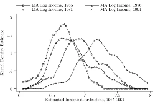
In figure 6 we move from analyzing the moments of the cross-state income distribu-tion over time, to looking directly at the distribudistribu-tion itself. Using the semi-parametric Epanechnikov kernel, we estimate the cross-state income distribution in 1966, 1976, 1981 and 1991.35 Following the convention in the literature, the bandwidth is calculated ‘opti-mally’.36 For the kernel density estimates we do not use the normalized income measure because it is interesting to visualize if the country-wide income distribution shifts to the right over time. In fact, this is thefirst thing we notice — that, on average, incomes in all states have increased over time. The second striking feature is the spreading out of the distribution — although this is not unexpected given the evidence in figure 4. In figure
3 3The box in the middle of each box plot describes the central tendencies of a distribution. The thin
line inside the box is the median; the top and bottom lines of the box are the 75th and 25th percentile respectively. The rays emanating from the box reach the upper and lower adjacent values. If the inter-quartile range isr, then the upper adjacent value is the largest income value observed no greater than the 75th percentile plus1.5×r. The lower adjacent value is similarly defined, extending downwards from the 25th percentile. From a purely statistical perspective, observations that lie outside the upper and lower adjacent values might be considered outliers.
3 4Thisnormalizedmeasure of log state real income per capita is calculated for each stateifor any given
year as follows
log( MA of real per capita income of statei
N−1ΣN
i=1real per capita income of statei
)
whereN is the total number of states in the sample.
3 5Some researchers, for example Sala-i-Martin (2002), use the Gaussian kernel. I also estimated all the
densities with the Gaussian kernel, and the identical bandwidth. The results were almost identical, and so are not reported here. In any case, for most purposes the choice of kernel is not as important as the choice of bandwidth.
3 6
The ‘optimal’ bandwidth is calculated using the formula bw= 0.9m
n15
where
m= min
µ√
variancex,interquartile rangex
1.349
Tukey Box Plot: Log Income relative to Sample Average -.5 0 .5 1961 1966 1971 15 1976 1981 1986 1991
Figure 5: DISPERSION OF THE CROSS-STATE INCOME DISTRIBUTION
Kernel Density
E
stim
a
te
Estimated Income distributions, 1965-1992
MA Log Income, 1966 MA Log Income, 1976 MA Log Income, 1981 MA Log Income, 1991
6 6.5 7 7.5 8 0 .5 1 1.5 2
6 it can be seen that the distribution becomes fatter over time, and the ‘primary’ mode of the distribution has become smaller. This is evidence of the increased dispersion or polarization within the cross-state income distribution. The third point of interest is the possible emergence of a second mode in the distribution towards the high income end. This is most obviously visible in the density estimates of 1976 and 1981.37 In 1991, even with the second mode, the right tail is considerably fatter. Overall, this suggests that at least part of theσ−divergence that we have documented so far can be attributed to an emerging multimodality — perhaps because a small group of states at the higher end of the income distribution is pulling away from the rest.38
Closer analysis of the income distribution reveals the identity of this elite group of states. Between 1965 and 1992, the two agricultural powerhouse states Punjab (state==15) and Haryana (state==5), along with the industrialized Maharashtra (state==11) have been consistent members of the top 25% of the income distribution.39 In the same period, these are the only 3 states in the sample which have clocked a growth rate in excess of 3%. That these rich states have grown as fast, and on occasion faster than the sample average, has ensured that their place at the top of the income distribution has been main-tained, and may be one of the key reasons why we found little evidence of unconditional
β−convergence in the last section.
However, this picture of the rich growing richer is by no means the whole story. West Bengal (state==21) was the richest state in 1960, but by the early 1990s it had fallen behind to sixth position in the income distribution. The two states which had edged ahead were Gujarat (state==4) and Tamil Nadu (state==18). Gujarat had been an early favorite — an above average industrialized state, geographically contiguous to Maharashtra (state==11) and renowed for its entrepreneurial workforce — it grew especially rapidly in the 1980s and 1990s in a more liberal industrial policy environment. By contrast, Tamil Nadu overtook West Bengal in terms of levels of income only in the early 1990s. In fact, Tamil Nadu (state==18) is one of a group of three southern Indian states which grew extremely rapidly in 1980s and continued growing strongly in the 1990s. For example in the decade of the 1980s, per capita income in Karnataka grew by 3.5%, in Tamil Nadu by 4.5%, and in Andhra Pradesh at the relatively dizzying rate of 5%. Consequently, all three states are, as of the mid-1990s, firmly ensconced in the top half of the cross-state income distribution. Together, Andhra Pradesh (state==1), Karnataka (state==8) and Tamil Nadu (state==18) constitute the best evidence of convergence or catch-up that we
3 7Bandyopadhyay (2001) documents the existence of twin-peaks in income in her study of distribution
dynamics across Indian states for a similar time period.
3 8
The possible multimodality infigure 4 is almost surely understated. It is well known that the ‘optimal’ bandwidth oversmoothes the density estimates in case the underlying true density is highly skewed or multimodal. (Pagan and Ullah, 1999, ch.2).
3 9In fact, using additional data on incomes between 1980 and 1996 (used in Trivedi (2000)), it is possible
St andard De vi at io n year
SD Log Income SD Log Popn Weighted Income
1965 1970 1975 1980 1985 1990
.2 .4 .6 .8
Figure 7: STANDARD DEVIATION OF THE CROSS-STATE INCOME DISTRIBUTION (RAW AND POPULATION WEIGHTED)
see in this period.
4.3
The Population Quali
fi
cation
Section 4.2 has documented the increasing income disparity between states over time. However, it would be erroneous to conclude, on the basis of this evidence, that individual income inequality has increased between 1960 and 1992. This is because the unit of comparison so far has been states rather than people. To move from making an analysis of inequality of income across states to drawing a conclusion about inequality of income across people is a complex research exercise, but it is possible to offer some preliminary insights based on some simple adjustments.
Figure 7 plots the standard deviation of the log of the population-weighted (real state per capita) income for the 16 states in the sample. For comparability, it also reports the unweighted measure shown infigure 4. Thefigure shows that in the standard deviation of the weighted measure, there is no clear upward trend over time, until about the mid-1980s after which the unweighted measure and the weighted measure seem to move together. (Note that no importance should be attached to the level of inequality shown in figure 7.) Since the population-weightedfigure implicitly assumes that all individuals in a given state have the same level of income, it obviously understates the true level of individual income inequality. In fact, even the trend as an indicator of individual income inequality
would be misleading if within-state income inequality changed significantly over time. If however, within-state income inequality did not change significantly over the period, then the movement in the standard deviation of the population-weighted measure of income would depict, more or less accurately, movements in individual income inequality.
At the all India level, there is some evidence that measured rural income inequality has fallen marginally between 1961 and 1992, but urban income inequality has not changed very much at all.40 A very similar pattern also holds at the state level.41 Hence, one can be reasonably confident about the trend movements in the population-weighted income measure. These suggest that the increasing cross-state income disparity between 1960 and 1992 did not lead to a corresponding increase in individual income inequality until 1985, after which there is a marked rise in both.
The dissonance between the standard deviation in the weighted and unweighted mea-sures before 1985 can be partly explained by the convergence of the numerically important southern states, which was referred to earlier. Together, Andhra Pradesh (state==1), Kar-nataka (state==8) and Tamil Nadu (state==18) make up approximately 21% of the total (sample) population. On the other hand, the co-movement of the variance of the weighted and unweighted measures post 1985 appears chiefly to be the result of a ‘growth collapse’ in Bihar (state==3) post 1985. Between 1961 and 1985 per capita income growth in Bihar was 1%. However, between 1985 and 1992, per capita income in Bihar contracted by -0.7%. Since Bihar is an important state in terms of population — in the sample of 16 states Bihar alone accounts for approximately 11% of the population — once it starts falling offthe graph after 1985 it induces an increase in the variance of both the weighted and the unweighted measures.42
5
Concluding Remarks
The stated aim of this paper was to provide a comprehensive empirical account of conver-gence and catch-up among the major states within India between 1960 and 1992. At least four important conclusions from can be noted from the empirical results presented. First, there is no evidence of unconditionalβ−convergence. In contrast to some previous studies we find no tendency for initially poorer states to grow faster. Different estimators were used to confirm that thisfinding is robust, in the sense that it holds across time periods,
4 0
Drèze and Sen (1995) report that between 1960-61 and 1990-91, the Gini coefficient for rural income inequality has fallen from 33 to 28; while the Gini coefficient for urban income inequality has fallen from 35.6 to 34.
4 1
Analyzing the state-level rural Gini coefficients reveals that of the all states,five had small statistically significant time trends, all negative. For the urban Gini coefficients, there were three states with small statistically significant time trends, two positive and one negative.
4 2
Bihar’s ‘growth collapse’ has continued well into the 1990s. Between 1990 and 1996, Bihar’s State Domestic Product contracted by approximately -0.02%.
and is not sensitive to outliers or variations in sample size. An equally robust finding is the existence of conditional β−convergence. After holding constant proxies for educa-tional and non-educaeduca-tional human capital, and physical capital, initially poorer states do converge faster to their differing steady-states. The addition offixed effects reinforces the conditional convergence effect, and highlights the importance of initial conditions to the future growth experiences across states. A third conclusion is thefinding ofσ−divergence. Analysis of measures of dispersion and the shape of the cross-state income distribution, show that over time, state incomes are moving further away from each other. It also appears that a small group of states is pulling away from the rest, resulting in an incip-ient second peak in the income distribution, although this will only be completely clear as we get data for future years. Thefinal conclusion cautions that the increased income disparities between states do not always imply increased personal income inequality in the whole country. However, the evidence does suggest that from the mid-1980s both kinds of income inequality might have risen.
These overall oraverage trends are instructive, but they are not the complete story. It is equally important and interesting to pinpoint what lies behind them. Throughout the paper, the analysis has tried to identify particular states which might be responsible, to a greater degree than others, for generating these aggregate patterns in the data. In so doing, we have uncovered examples of catching-up and falling behind within the income distribution, at the same time as movements towards greater polarization at both the extremities of the income distribution.
A
Data and Sources
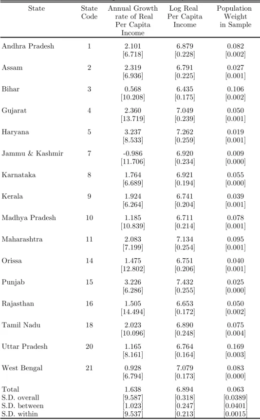
The data set covers the 16 major states of India, in most cases for a period of 32 years, between 1960 and 1992. Most of these states were reorganized along linguistic lines to currently specified boundaries in 1956,43 and have existed as such until the year 2000.44 In 1960 Bombay State was split into Gujarat and Maharashtra. In 1965-66 the core Punjabi Suba was split up into Punjab, Haryana and Himachal Pradesh; and data for both Punjab and Haryana commences in 1965 for most variables. Data on Jammu and Kashmir is patchy in the early years and in the early 1990s for most explanatory variables in the conditional convergence regressions of table II. Hence it is dropped from the sample under estimation for table II. Out of the 16 states, it is the smallest and not of special economic significance either. In this limited statistical sense, it is the least painful to omit. Table A-1 below provides a list of the states in the sample with the average per capita income, and the average annual growth rate of per capita income during the sample period.
4 3
The States Reorganisation act, 1956, specified 14 states within the Indian Union. For more on the linguistic reorganisation of states in India, see Paul Brass (1990).
4 4
In the year 2000, three of the states in the sample were bifurcated. Uttaranchal, Jharkhand, and Chattisgarh were carved out of Uttar Pradesh, Bihar and Madhya Pradesh, respectively.
State State Annual Growth Log Real Population Code rate of Real Per Capita Weight
Per Capita Income in Sample Income Andhra Pradesh 1 2.101 6.879 0.082 [6.718] [0.228] [0.002] Assam 2 2.319 6.791 0.027 [6.936] [0.225] [0.001] Bihar 3 0.568 6.435 0.106 [10.208] [0.175] [0.002] Gujarat 4 2.360 7.049 0.050 [13.719] [0.239] [0.001] Haryana 5 3.237 7.262 0.019 [8.533] [0.259] [0.001] Jammu & Kashmir 7 -0.986 6.920 0.009
[11.706] [0.234] [0.000] Karnataka 8 1.764 6.921 0.055 [6.689] [0.194] [0.000] Kerala 9 1.924 6.741 0.039 [6.264] [0.204] [0.001] Madhya Pradesh 10 1.185 6.711 0.078 [10.839] [0.214] [0.001] Maharashtra 11 2.083 7.134 0.095 [7.199] [0.254] [0.001] Orissa 14 1.475 6.751 0.040 [12.802] [0.206] [0.001] Punjab 15 3.226 7.432 0.025 [6.286] [0.255] [0.000] Rajasthan 16 1.505 6.653 0.050 [14.494] [0.172] [0.002] Tamil Nadu 18 2.023 6.890 0.075 [10.096] [0.248] [0.004] Uttar Pradesh 20 1.165 6.764 0.169 [8.161] [0.164] [0.003] West Bengal 21 0.928 7.079 0.083 [6.794] [0.173] [0.000] Total 1.638 6.894 0.063 S.D. overall [9.587] [0.318] [0.0389] S.D. between [1.023] [0.247] [0.0401] S.D. within [9.537] [0.213] [0.0015]
Table A-1: Summary Characteristics (1960-1992)
A.1
Income/Growth
The two sources for the incomes data are
• Ozler, Datt, and Ravallion (1996): This data set compiles a consistent set of figures on incomes, price indices, population, inter alia for the rural and urban areas of India’s sixteen major states spanning the period 1958-1992.
• Estimates of the State Domestic Product, Central Statistical Organization, various issues. Estimates after 1981 are from diskettes obtained directly from the CSO office, Sardar Patel Bhavan, New Delhi.
Real state per capita income is calculated in the following manner. A deflator is con-structed using different price indices for agricultural labourers (scpial1) and industrial workers(stcpiw1) by state and year from the Ozler et al(1996) data set, and by weigh-ing them by the respective rural and urban population shares (pop1 and pop2). The population data comes from the decennial census estimates. Between any two censuses it is assumed to grow at a constant rate of growth derived from the respective population totals. Like almost all other variables in the paper the deflator is also time-varying and state-varying.
def latori,t= pop 1
pop1+pop2 ×scpial1+
pop2
pop1+pop2×stcpiw1
Estimates of the Net State Domestic Product (computed at factor cost and current prices) for each state and all sectors and year are then divided by the total population and the deflator to obtain consistent estimates of real state per capita income. Growth rates are calculated by taking log differences of the real state per capita income, and divided by the number of intervening years.
A.2
Education Measures
High School enrollment data comes from the serial publication, Education in India, De-partment of Education, Government of India. The data relates to boys and girls between 11 and 14 years of age. The enrollment rates are calculated as the percentage of students enrolled in classes 6 — 8 to the estimated child population in the age group 11 to 14. Schooling in this age group is sometimes also categorized as ‘upper primary’.
A.3
The Infant Mortality Rate
Data on infant mortality rates from the Sample Registration Survey (SRS) was collected from various issues of theSample Registration Bulletin, Office of the Registrar General, Government of India; and from Bose, A.,India’s Basic Demographic Statistics: 177 Key