Learning Feature Selection Dependencies in
Multi-task Learning
Daniel Hern´andez-Lobato Computer Science Department Universidad Aut´onoma de Madrid [email protected]
Jos´e Miguel Hern´andez-Lobato Department of Engineering
University of Cambridge [email protected]
Abstract
A probabilistic model based on the horseshoe prior is proposed for learning de-pendencies in the process of identifying relevant features for prediction. Exact inference is intractable in this model. However, expectation propagation offers an approximate alternative. Because the process of estimating feature selection dependencies may suffer from over-fitting in the model proposed, additional data from a multi-task learning scenario are considered for induction. The same model can be used in this setting with few modifications. Furthermore, the assumptions made are less restrictive than in other multi-task methods: The different tasks must share feature selection dependencies, but can have different relevant features and model coefficients. Experiments with real and synthetic data show that this model performs better than other multi-task alternatives from the literature. The experiments also show that the model is able to induce suitable feature selection dependencies for the problems considered, only from the training data.
1
Introduction
Many linear regression problems are characterized by a large numberdof features or explaining attributes and by a reduced numbern of training instances. In this largedbut smallnscenario there is an infinite number of potential model coefficients that explain the training data perfectly well. To avoid over-fitting problems and to obtain estimates with good generalization properties, a typical regularization is to assume that the model coefficients are sparse,i.e., most coefficients are equal to zero [1]. This is equivalent to considering that only a subset of the features or attributes are relevant for prediction. The sparsity assumption can be introduced by carrying out Bayesian inference under a sparsity enforcing prior for the model coefficients [2, 3], or by minimizing a loss function penalized by some sparse regularizer [4, 5]. Among the priors that enforce sparsity, the horseshoe has some attractive properties that are very convenient for the scenario described [3]. In particular, this prior has heavy tails, to model coefficients that significantly differ from zero, and an infinitely tall spike at the origin, to favor coefficients that take negligible values.
The estimation of the coefficients under the sparsity assumption can be improved by introducing dependencies in the process of determining which coefficients are zero [6, 7]. An extreme case of these dependencies appears in group feature selection methods in which groups of coefficients are considered to be jointly equal or different from zero [8, 9]. However, a practical limitation is that the dependency structure (groups) is often assumed to be given. Here, we propose a model based on the horseshoe prior that induces the dependencies in the feature selection process from the training data. These dependencies are expressed by a correlation matrix that is specified byO(d)parameters. Unfortunately, the estimation of these parameters from the training data is difficult since we consider
n < dinstances only. Thus, over-fitting problems are likely to appear. To improve the estimation process we assume a multi-task learning setting, where several learning tasks share feature selection dependencies. The method proposed can be adapted to such a scenario with few modifications.
Traditionally, methods for multi-task learning under the sparsity assumption have considered com-mon relevant and irrelevant features acom-mong tasks [8, 10, 11, 12, 13, 14]. Nevertheless, recent re-search cautions against this assumption when the supports and values of the coefficients for each task can vary widely [15]. The model proposed here limits the impact of this problem because it is has fewer restrictions. The tasks used for induction can have, besides different model coefficients, different relevant features. They must share only the dependency structure for the selection process. The model described here is most related to the method for sparse coding introduced in [16], where spike-and-slab priors [2] are considered for multi-task linear regression under the sparsity assump-tion and dependencies in the feature selecassump-tion process are specified by a Boltzmann machine. Fitting exactly the parameters of a Boltzmann machine to the observed data has exponential cost in the num-ber of dimensions of the learning problem. Thus, when compared to the proposed model, the model considered in [16] is particularly difficult to train. For this, an approximate algorithm based on block-coordinate optimization has been described in [17]. The algorithm alternates between greedy MAP estimation of the sparsity patterns of each task and maximum pseudo-likelihood estimation of the Boltzmann parameters. Nevertheless, this algorithm lacks a proof of convergence and we have observed that is prone to get trapped in sub-optimal solutions.
Our experiments with real and synthetic data show the better performance of the model proposed when compared to other methods that try to overcome the problem of different supports among tasks. These methods include the model described in [16] and the model for dirty data proposed in [15]. These experiments also illustrate the benefits of the proposed model for inducing depen-dencies in the feature selection process. Specifically, the dependepen-dencies obtained are suitable for the multi-task learning problems considered. Finally, a difficulty of the model proposed is that exact Bayesian inference is intractable. Therefore, expectation propagation (EP) is employed for efficient approximate inference. In our model EP has a cost that isO(Kn2d), whereK is the number of
learning tasks,nis the number of samples of each task, anddis the dimensionality of the data. The rest of the paper is organized as follows: Section 2 describes the proposed model for learning feature selection dependencies. Section 3 shows how to use expectation propagation to approximate the quantities required for induction. Section 4 compares this model with others from the literature on synthetic and real data regression problems. Finally, Section 5 gives the conclusions of the paper and some ideas for future work.
2
A Model for Learning Feature Selection Dependencies
We describe a linear regression model that can be used for learning dependencies in the process of identifying relevant features or attributes for prediction. For simplicity, we first deal with the case of a single learning task. Then, we show how this model can be extended to address multi-task learning problems. In the single multi-task scenario we consider some training data in the form of
n d-dimensional vectors summarized in a design matrixX= (x1, . . . ,xn)Tand associated targets
y = (y1, . . . , yn)T, with yi ∈ R. A linear predictive rule is assumed for ygivenX. Namely,
y=Xw+, wherewis a vector of latent coefficients andis a vector of independent Gaussian noise with varianceσ2,i.e.,∼ N(0, σ2I). GivenXandy, the likelihood forwis:
p(y|X,w) = n Y i=1 p(yi|xi,w) = n Y i=1 N(yi|wTxi, σ2) =N(y|Xw, σ2I). (1) Consider the under-determined scenarion < d. In this case, the likelihood is not strictly concave and infinitely many values ofwfit the training data perfectly well. A strong regularization technique that is often used in this context is to assume that only some features are relevant for prediction [1]. This is equivalent to assuming thatwis sparse with many zeros. This inductive bias can be naturally incorporated into the model using a horseshoe sparsity enforcing prior forw[3].
The horseshoe prior lacks a closed form but can be defined as a scale mixture of Gaussians:
p(w|τ) = d Y j=1 p(wj|τ), p(wj|τ) = Z N(wj|0, λ2jτ2)C+(λj|0,1)dλ j, (2)
whereλjis a latent scale for coefficientwj,C+(·|0,1)is a half-Cauchy distribution with zero loca-tion and unit scale andτ >0is aglobalshrinkage parameter that controls the level of sparsity. The
smaller the value ofτthe sparser the prior and vice-versa. Figure 1 (left) and (middle) show a com-parison of the horseshoe with other priors from the literature. The horseshoe has an infinitely tall spike at the origin which favors coefficients with small values, and has heavy tails which favor co-efficients that take values that significantly differ from zero. Furthermore, assume thatτ =σ2= 1
and thatX=I, and defineκj= 1/(1 +λ2j). Then, the posterior mean forwjis(1−κj)yj, where
κjis a random shrinkage coefficient that can be interpreted as the amount of weight placed at the origin [3]. Figure 1 (right) shows the prior density forκjthat results from the horseshoe. It is from the shape of this figure that the horseshoe takes its name. We note that one expects to see two things under this prior: relevant coefficients (κj ≈0, no shrinkage), and zeros (κj ≈1, total shrinkage). The horseshoe is therefore very convenient for the sparse inducing scenario described before.
−3 −2 −1 0 1 2 3 0.0 0.1 0.2 0.3 0.4 0.5 0.6 0.7 Prob .Density Horseshoe Gaussian Student−t(df=1) Laplace 4 5 6 7 0.000 0.005 0.0 10 0.015 0.020 0.025 Prob .Density Horseshoe Gaussian Student−t(df=1) Laplace 0.0 0.2 0.4 0.6 0.8 1.0 0 1 2 3 4 5 Prob .Density
Figure 1: (left) Density of different priors, horseshoe, Gaussian, Student-t and Laplace near the origin. Note the infinitely tall spike of the horseshoe. (middle) Tails of the different priors considered before. (right) Prior density of the shrinkage parameterκjfor the horseshoe prior.
A limitation of the horseshoe is that it does not consider dependencies in the feature selection pro-cess. Specifically, the fact that one feature is actually relevant for prediction has no impact at all in the prior relevancy or irrelevancy of other features. We now describe how to introduce these dependencies in the horseshoe. Consider the definition of a Cauchy distribution as the ratio of two independent standard Gaussian random variables [18]. An equivalent representation of the prior is:
p(w|ρ2, γ2) =
Z d
Y
j=1
N(wj|0, u2j/vj2)N(uj|0, ρ2)N(vj|0, γ2)dujdvj. (3) whereujandvjare latent variables introduced for each dimensionj. In particular,λj =ujγ/vjρ. Furthermore, τ has been incorporated into the prior foruj andvj using τ2 = ρ2/γ2. The latent variablesujandvjcan be interpreted as indicators of the relevance or irrelevance of featurej. The largeru2
j, the more relevant the feature. Conversely, the largerv2j, the more irrelevant.
A simple way of introducing dependencies in the feature selection process is to consider correlations among variablesujandvj, withj= 1, . . . , d. These correlations can be introduced in (3) as follows:
p(w|ρ2, γ2,C) = Z d Y j=1 N(wj|0, u2j/v2j) N(u|0, ρ 2C) N(v|0, γ2C)dudv, (4) whereu= (u1, . . . , ud)T,v= (v1, . . . , vd)T,Cis a correlation matrix that specifies the dependen-cies in the feature selection process, andρ2andγ2act as regularization parameters that control the
level of sparsity. WhenC=I, (4) factorizes and gives the same prior as the one in (2) and (3). In practice, however,Chas to be estimated from the data. This can be problematic since it will involve the estimation ofO(d2)free parameters which can lead to over-fitting. To alleviate this problem and
also to allow for efficient approximate inference we consider a special form forC:
C=∆M∆, M= (D+PPT), ∆=diag(1/pM11, . . . ,1/
p
Mdd), (5) where diag(a1, . . . , ad)denotes a diagonal matrix with entriesa1, . . . , ad;Dis a diagonal matrix whose entries are all equal to some small positive constant (this matrix guarantees thatC−1exists);
the products by∆ensure that the entries ofCare in the range(−1,1); andPis ad×mmatrix of real entries which specifies the correlation structure ofC. Thus,Cis fully determined byPand will only haveO(md)free parameters withm < d. The value ofmis a regularization parameter that limits the complexity ofC. The larger its value, the more expressiveCis. For computational reasons described later on we will set in our experimentsmequal ton, the number of data instances.
2.1 Inference, Prediction and Learning Feature Selection Dependencies
Denote byz= (wT,uT,vT)Tthe vector of latent variables of the model described above. Based on the formulation of the previous section, the joint probability distribution ofyandzis:
p(y,z|X, σ2, ρ2, γ2,C) =N(y|Xw, σ2I)N(u|0, ρ2C)N(v|0, γ2C)
d
Y
j=1
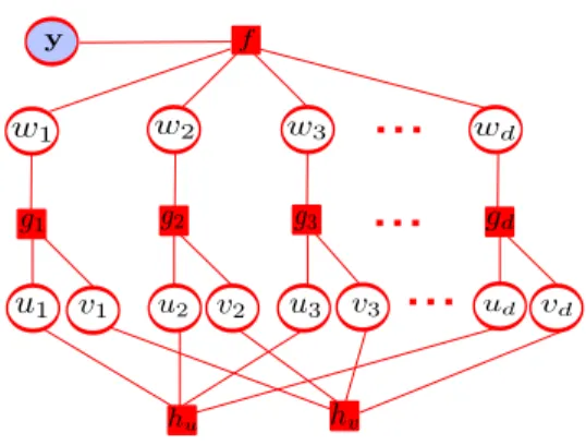
N wj|0, u2j/vj2. (6) Figure 2 shows the factor graph corresponding to this joint probability distribution. This graph summarizes the interactions between the random variables in the model. All the factors in (6) are Gaussian, except the ones corresponding to the prior forwjgivenujandvj,N(wj|0, u2j/v2j). Given the observed targetsy one is typically interested in inferring the latent variables zof the model. For this, Bayes’ theorem can be used:
p(z|X,y, σ2, ρ2, γ2,C) = p(y,z|X, σ
2, ρ2, γ2,C)
p(y|X, σ2, ρ2, γ2,C) , (7)
where the numerator in the r.h.s. of (7) is the joint distribution (6) and the denominator is simply a normalization constant (the model evidence) which can be used for Bayesian model selection [19]. The posterior distribution in (7) is useful to compute a predictive distribution for the target ynew associated to a new unseen data instancexnew:
p(ynew|xnew,X, σ2, ρ2, γ2,C) =
Z
p(ynew|xnew,w)p(z|X, σ2, ρ2, γ2,C)dz. (8) Similarly, one can marginalize (7) with respect tow to obtain a posterior distribution foruandv
which can be useful to identify the most relevant or irrelevant features.
...
...
...
Figure 2: Factor graph of the probabilistic
model. The factor f(·) corresponds to the
likeli-hood N(y|Xw, σ2I), and each gj(·) to the prior
forwjgiven uj andvj, N(wj|0, u2j/v2j). Finally,
hu(·) and hv(·) correspond to N(u|0, ρ2C) and
N(v|0, γ2C)
, respectively. Only the targetsy are
observed, the other variables are latent.
Ideally, however, one should also inferC, the cor-relation matrix that describes the dependencies in the feature selection process, and compute a pos-terior distribution for it. This can be complicated, even for approximate inference methods. Denote byZthe model evidence,i.e., the denominator in the r.h.s. of (7). A simpler alternative is to use gradient ascent to maximizelogZ (and therefore
Z) with respect toP, the matrix that completely specifies C. This corresponds to type-II maxi-mum likelihood (ML) estimation and allows to determinePfrom the training data alone, without resorting to cross-validation [19]. The gradient of
logZ with respect toP,i.e.,∂logZ/∂Pcan be used for this task. The other hyper-parameters of the modelσ2,ρ2andγ2can be found following
a similar approach.
Unfortunately, neither (7), (8) nor the model ev-idence can be computed in closed form. Specif-ically, it is not possible to compute the required integrals analytically. Thus, one has to resort to approximate inference. For this, we use expecta-tion propagaexpecta-tion [20]. See Secexpecta-tion 3 for details. 2.2 Extension to the Multi-Task Learning Setting
In the single-task learning setting maximizing the model evidence with respect toPis not expected to be effective to improve the prediction accuracy. The reason is the difficulty of obtaining an ac-curate estimate ofP. This matrix hasm×dfree parameters and these have to be induced from a small number ofn < dtraining instances. The estimation process is hence likely to be affected by over-fitting. One way to mitigate over-fitting problems is to consider additional data for the estima-tion process. These addiestima-tional data may come from a multi-task learning setting, where there areK
related but different tasks available for induction. A simple assumption is that all these tasks share a common dependency structureCfor the feature selection process, although the model coefficients and the actual relevant features may differ between tasks. This assumption is less restrictive than as-suming jointly relevant and irrelevant features across tasks and can be incorporated into the learning process using the described model with few modifications. By using the data from theKtasks for the estimation ofPwe expect to obtain better estimates and to improve the prediction accuracy. Assume there areKlearning tasks available for induction and that each taskk= 1, . . . , Kconsists of a design matrixXkwithnkd-dimensional data instances and target valuesyk. As in (1), a linear predictive rule with additive Gaussian noiseσ2
k is considered for each task. Letwk be the model coefficients of taskk. Assume for the model coefficients of each task a horseshoe prior as the one specified in (4) with a shared correlation matrixC, but with task specific hyper-parametersρ2kand
γ2
k. Denote byukandvkthe vectors of latent Gaussian variables of the prior for taskk. Similarly, let
zk= (wkT,u T k,v
T k)
Tbe the vector of latent variables of taskk. Then, the joint posterior distribution of the latent variables of the different tasks factorizes as follows:
p {z}K k=1|{Xk,yk, τk2, ρ 2 k, σ 2 k} K k=1,C = K Y k=1 p(yk,zk|Xk, σ2k, ρ 2 k, γ 2 k,C) p(yk|Xk, σ2k, ρ2k, γk2,C) , (9)
where each factor in the r.h.s. of (9) is given by (7). This indicates that theKmodels for each task can be learnt independently givenCandσ2
k,ρ
2
kandγ
2
k ∀k. Denote byZMTthe denominator in the r.h.s. of (9),i.e.,ZMT=Q
K
k=1p(yk|Xk, σk2, ρ2k, γ2k,C) =
QK
k=1Zk, withZk the evidence for task
k. Then,ZMTis the model evidence for the multi-task setting. As in single-task learning, specific values for the hyper-parameters of each task andCcan be found by a type-II maximum likelihood (ML) approach. For this,logZMT is maximized using gradient ascent. Specifically, the gradient of logZMTwith respect to σk2, ρ
2
k,γ
2
k andPcan be easily computed in terms of the gradient of eachlogZk. In summary, if there is a method to approximate the required quantities for learning a single task using the model proposed, implementing a multi-task learning method that assumes shared feature selection dependencies but task dependent hyper-parameters is straight-forward.
3
Approximate Inference
Expectation propagation (EP) [20] is used to approximate the posterior distribution and the evidence of the model described in Section 2. For the clarity of presentation we focus on the model for a single learning task. The multi-task extension of Section 2.2 is straight-forward. Consider the posterior distribution ofz, (6). Up to a normalization constant this distribution can be written as
p(z|X,y, σ2, ρ2, γ2)∝f(w)hu(u)hv(v) d
Y
j=1
gj(z), (10)
where the factors in the r.h.s. of (10) are displayed in Figure 2. Note that all factors except thegj’s are Gaussian. EP approximates (10) by a distributionq(z)∝f(w)hu(u)hv(v)Q
d
j=1g˜j(z), which is obtained by replacing each non-Gaussian factorgj in (10) with an approximate factorg˜j that is Gaussian but need not be normalized. Since the Gaussian distribution belongs to the exponential family of distributions, which is closed under the product and division operations [21],qis Gaussian with natural parameters equal to the sum of the natural parameters of each factor.
EP iteratively updates eachg˜j until convergence by first computingq\j ∝q/˜gjand then minimiz-ing the Kullback-Leibler (KL) divergence betweengjq\jandqnew, KL(gjq\j||qnew), with respect to
qnew. The new approximate factor is obtained asg˜new
j =sjqnew/q\j, wheresjis the normalization constant ofgjq\j. This update rule ensures that˜gj looks similar togj in regions of high posterior probability in terms ofq\j[20]. Minimizing the KL divergence is a convex problem whose optimum is found by matching the means and the covariance matrices betweengjq\j andqnew. These expec-tations can be readily obtained from the derivatives oflogsj with respect to the natural parameters ofq\j[21]. Unfortunately, the computation ofsjis intractable under the horseshoe. As a practical alternative, our EP implementation employes numerical quadrature to evaluatesjand its derivatives. Importantly,gj, and thereforeg˜j, depend only onwj,ujandvj, so a three-dimensional quadrature
will suffice. However, using similar arguments to those in [7] more efficient alternatives exist. As-sume thatq\j(w
j, uj, vj) =N(wj|mj, ηj)N(uj|0, νj)N(vj|0, ξj),i.e.,q\jfactorizes with respect towj,uj andvj and that the mean ofujandvjis zero. Sincegjis symmetric with respect touj andvjthenE[uj] =E[vj] =E[ujvj] =E[ujwj] =E[vjwj] = 0undergjq\j. Thus, if the initial approximate factorsg˜jfactorize with respect towj,ujandvj, and have zero mean with respect to
ujandvj, any updated factor will also satisfy these properties andq\jwill have the assumed form. The crucial point here is that the dependencies introduced bygjdo not lead to correlations that need to be tracked under a Gaussian approximation. In this situation, the integral ofgjq\jwith respect to
wjis given by the convolution of two Gaussians and the integral of the result with respect toujand
vjcan be simplified using arguments similar to those employed to obtain (3). Namely,
sj= Z N mj|0, νj ξj λ2j+ηj C+(λj|0,1)dλ j, (11)
wheremj,ηj,νj andξj are the parameters ofq\j. The derivatives oflogsj with respect to the natural parameters ofq\j can also be evaluated using a one-dimensional quadrature. Therefore, each update of˜gjrequires five quadratures: one to evaluatesjand four to evaluate its derivatives. Instead of sequentially updating eachg˜j, we follow [7] and update these factors in parallel. For this, we compute allq\j at the same time and update eachg˜
j. The marginals ofqare strictly required for this task. These can be efficiently obtained using the low rank representation structure of the covariance matrix ofqthat results from the fact that all theg˜j’s are factorizing univariate Gaussians and from the assumed form forCin (5). Specifically, ifm(the number of columns ofP) is equal ton, the cost of this operation (and hence the cost of EP) isO(n2d). Lastly, we damp the update of eachg˜jas follows:˜gj= (˜gnewj )α(˜goldj )1−α, whereg˜newj andg˜joldrespectively denote the new and the old˜gj, andα∈ [0,1]is a parameter that controls the amount of damping. Damping significantly improves the convergence of EP and leaves the fixed points of the algorithm invariant [22].
After EP has converged,q can be used instead of the exact posterior in (8) to make predictions. Similarly, the model evidence in (7) can be approximated byZ˜, the normalization constant ofq:
˜ Z= Z f(w)hu(u)hv(v) d Y j=1 ˜ gj(z)dwdudv. (12)
Since all the factors in (12) are Gaussian,log ˜Zcan be readily computed and maximized with respect toσ2, ρ2, γ2 andPto find good values for these hyper-parameters. Specifically, once EP has converged, the gradient of the natural parameters of the˜gj’s with respect to these hyper-parameters is zero [21]. Thus, the gradient oflog ˜Zwith respect toσ2,ρ2,γ2andPcan be computed in terms of the gradient of the exact factors. The derivations are long and tedious and hence omitted here, but by careful consideration of the covariance structure ofqit is possible to limit the complexity of these computations toO(n2d)ifmis equal ton. Therefore, to fit a model that maximizeslog ˜Zwe
alternate between running EP to obtain the estimate oflog ˜Zand its gradient, and doing a gradient ascent step to maximize this estimate with respect toσ2,ρ2,γ2andP. The derivation details of the
EP algorithm and an R-code implementation of it can be found in the supplementary material.
4
Experiments
We carry out experiments to evaluate the performance of the model described in Section 2. We refer to this model as HSDep. Other methods from the literature are also evaluated. The first one, HSST, is a particular case of HSDepthat is obtained when each task is learnt independently and correlations in the feature selection process are ignored (i.e.,C=I). A multi-task learning model, HSMT, which assumes common relevant and irrelevant features among tasks is also considered. The details of this model are omitted, but it follows [10] closely. It assumes a horseshoe prior in which the scale parametersλjin (2) are shared among tasks,i.e., each feature is either relevant or irrelevant inall tasks. A variant of HSM T, SSMT, is also evaluated. SSMTconsiders a spike-and-slab prior for joint feature selection across all tasks, instead of a horseshoe prior. The details about the prior of SSMT are given in [10]. EP is used for approximate inference in both HSMTand SSMT. Thedirty model, DM, described in [15] is also considered. This model assumes shared relevant and irrelevant features
among tasks. However, some tasks are allowed to have specific relevant features. For this, a loss function is minimized via combined`1and`1/`∞block regularization. Particular cases of DM are
the lasso [4] and the group lasso [8]. Finally, we evaluate the model introduced in [16]. This model, BM, uses spike-and-slab priors for feature selection and specifies dependencies in this process using a Boltzmann machine. BM is trained using the approximate block-coordinate algorithm described in [17]. All models considered assume Gaussian additive noise around the targets.
4.1 Experiments with Synthetic Data
A first batch of experiments is carried out using synthetic data. We generate K = 64 dif-ferent tasks of n = 64 samples and d = 128 features. In each task, the entries of Xk are sampled from a standard Gaussian distribution and the model coefficients, wk, are all set to zero except for the i-th group of 8 consecutive coefficients, with i chosen randomly for each task from the set {1,2, . . . ,16}. The values of these 8 non-zero coefficients are uniformly dis-tributed in the interval [−1,1]. Thus, in each task there are only 8 relevant features for pre-diction. Given each Xk and each wk, the targets yk are obtained using (1) with σ2k = 0.5 ∀k. The hyper-parameters of each method are set as follows: In HSST ρ2k and γk2 are found
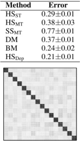
Method Error HSST 0.29±0.01 HSMT 0.38±0.03 SSMT 0.77±0.01 DM 0.37±0.01 BM 0.24±0.02 HSDep 0.21±0.01
Figure 3: (top) Average recon-struction error of each method. (bottom) Average absolute value
of the entries of the matrixC
es-timated by HSDep in gray scale
(white=0 and black=1). Black
squares are groups of jointly rel-evant / irrelrel-evant features.
by type-II ML. In HSMTρ2andγ2are set to the average value found by HSSTforρ2k andγk2, respectively. In SSMTthe parameters of the spike-and-slab prior are found by type-II ML. In HSDep m = n. Furthermore,ρ2kandγk2take the values found by HSSTwhilePis obtained using type-II ML. In all models we set the variance of the noise for taskk,σ2
k, equal to0.5. Finally, in DM we try different hyper-parameters and report the best results observed. After train-ing each model on the data, we measure the average reconstruction error ofwk. Denote bywˆk the estimate of the model coefficients for taskk(this is the posterior mean except in BM and DM). The reconstruction error is measured as||wˆk−wk||2/||wk||2, where
|| · ||2is the`2-norm andwk are the exact coefficients of taskk. Figure 3 (top) shows the average reconstruction error of each method over50repetitions of the experiments described. HSDep ob-tains the lowest error. The observed differences in performance are significant according to a Student’st-test (p-value<5%). BM per-forms worse than HSDepbecause the greedy MAP estimation of the sparsity patterns of each task is sometimes trapped in sub-optimal solutions. The poor results of HSMT, SSMTand DM are due to the assumption made by these models ofalltasks sharing relevant fea-tures, which is not satisfied. Figure 3 (bottom) shows the average entries in absolute value of the correlation matrixCestimated by HSDep. The matrix has a block diagonal form, with blocks of size
8×8(8is the number of relevant coefficients in each task). Thus, within each block the corresponding latent variablesuj andvj are strongly correlated, indicating jointly relevant or irrelevant features. This is the expected estimation for the scenario considered.
4.2 Reconstruction of Images of Hand-written Digits from the MNIST
A second batch of experiments considers the reconstruction of images of hand-written digits ex-tracted from the MNIST data set [23]. These images are in gray scale with pixel values between 0 and 255. Most pixels are inactive and equal to 0. Thus, the images are sparse and suitable to be reconstructed using the model proposed. The images are reduced to size10×10pixels and the pixel intensities are normalized to lie in the interval[0,1]. Then,K= 100tasks ofn= 75samples each are generated. For this, we randomly choose50images corresponding to the digit3and50images corresponding to the digit5(these digits are chosen because they differ significantly). Similar results (not shown) to the ones reported here are obtained for other pairs of digits. For each task, the entries of Xk are sampled from a standard Gaussian. The model coefficients, wk, are simply the pixel values of each image (i.e.,d = 100). Importantly, unlike in the previous experiments, the model coefficients are not synthetically generated but correspond to actual images. Furthermore, since the
tasks contain images of different digits they are expected to have different relevant features. Given
Xkandwk, the targetsykare generated using (1) withσ2k= 0.1∀k. The objective is to reconstruct
wk fromXkandykfor each taskk. The hyper-parameters are set as in Section 4.1 withσ2k = 0.1 ∀k. The reconstruction error is also measured as in that section.
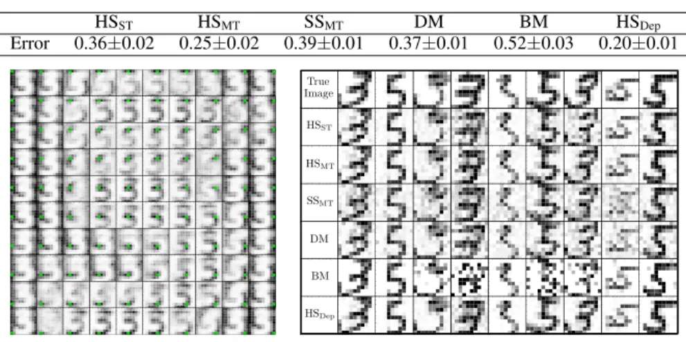
Figure 4 (top) shows the average reconstruction error of each method over50repetitions of the ex-periments described. Again, HSDepperforms best. Furthermore, the differences in performance are also statistically significant. The second best result corresponds to HSMT, probably due to back-ground pixels which are irrelevant in allthe tasks and to the heavy-tails of the horseshoe prior. HSST, SSM T, BM and DM perform significantly worse. DM performs poorly probably because of the inferior shrinking properties of the`1norm compared to the horseshoe [3]. The poor results of
SSMTare due to the lack of heavy-tails in the spike-and-slab prior. In BM we have observed that the greedy MAP estimation of the task supports is more frequently trapped in sub-optimal solutions. Furthermore, the algorithm described in [17] fails to converge most times in this scenario. Figure 4 (right, bottom) shows a representative subset of the images reconstructed by each method. The best reconstructions correspond to HSDep. Finally, Figure 4 (left, bottom) shows in gray scale the average correlations in absolute value induced by HSDepfor the selection process of each pixel of the image with respect to the selection of a particular pixel which is displayed in green. Correlations are high to avoid the selection of background pixels and to select pixels that actually correspond to the digits
3and5. The correlations induced are hence appropriate for the multi-task problem considered.
HSST HSMT SSMT DM BM HSDep Error 0.36±0.02 0.25±0.02 0.39±0.01 0.37±0.01 0.52±0.03 0.20±0.01 ● ● ● ● ● ● ● ● ● ● ● ● ● ● ● ● ● ● ● ● ● ● ● ● ● ● ● ● ● ● ● ● ● ● ● ● ● ● ● ● ● ● ● ● ● ● ● ● ● ● ● ● ● ● ● ● ● ● ● ● ● ● ● ● ● ● ● ● ● ● ● ● ● ● ● ● ● ● ● ● ● ● ● ● ● ● ● ● ● ● ● ● ● ● ● ● ● ● ● ●
Figure 4: (top) Average reconstruction error each method. (left, bottom) Average absolute value correlation in
a gray scale (white=0 and black=1) between the latent variablesujandvjcorresponding to the pixel displayed
in green and the variablesujandvjcorresponding to all the other pixels of the image. (right, bottom) Examples
of actual and reconstructed images by each method. The best reconstruction results correspond to HSDep.
5
Conclusions and Future Work
We have described a linear sparse model for learning dependencies in the feature selection process. The model can be used in a multi-task learning setting with several tasks available for induction that need not share relevant features, but only dependencies in the feature selection process. Exact inference is intractable in such a model. However, expectation propagation provides an efficient approximate alternative with a cost inO(Kn2d), whereKis the number of tasks,nis the number of samples of each task, anddis the dimensionality of the data. Experiments with real and synthetic data illustrate the benefits of the proposed method. Specifically, this model performs better than other multi-task alternatives from the literature. Our experiments also show that the proposed model is able to induce relevant feature selection dependencies from the training data alone. Future paths of research include the evaluation of this model in practical problems of sparse coding,i.e., when all tasks share a common design matrixXthat has to be induced from the data alongside with the model coefficients, with potential applications to image denoising and image inpainting [24]. Acknowledgment: Daniel Hern´andez-Lobato is supported by the Spanish MCyT (Ref. TIN2010-21575-C02-02). Jos´e Miguel Hern´andez-Lobato is supported by Infosys Labs, Infosys Limited.
References
[1] I. M. Johnstone and D. M. Titterington. Statistical challenges of high-dimensional data. Philosophical
Transactions of the Royal Society A: Mathematical, Physical and Engineering Sciences, 367(1906):4237,
2009.
[2] T. J. Mitchell and J. J. Beauchamp. Bayesian variable selection in linear regression. Journal of the
American Statistical Association, 83(404):1023–1032, 1988.
[3] C. M. Carvalho, N. G. Polson, and J. G. Scott. Handling sparsity via the horseshoe.Journal of Machine
Learning Research W&CP, 5:73–80, 2009.
[4] R. Tibshirani. Regression shrinkage and selection via the lasso.Journal of the Royal Statistical Society.
Series B (Methodological), 58(1):267–288, 1996.
[5] M. E. Tipping. Sparse Bayesian learning and the relevance vector machine.Journal of Machine Learning
Research, 1:211–244, 2001.
[6] J. M. Hern´andez-Lobato, D. Hern´andez-Lobato, and A. Su´arez. Network-based sparse Bayesian
classifi-cation.Pattern Recognition, 44:886–900, 2011.
[7] M. Van Gerven, B. Cseke, R. Oostenveld, and T. Heskes. Bayesian source localization with the multivari-ate Laplace prior. In Y. Bengio, D. Schuurmans, J. Lafferty, C. K. I. Williams, and A. Culotta, editors,
Advances in Neural Information Processing Systems 22, pages 1901–1909, 2009.
[8] Julia E. Vogt and Volker Roth. The group-lasso:`1,∞regularization versus`1,2regularization. In Goesele
et al., editor,32nd Anual Symposium of the German Association for Pattern Recognition, volume 6376,
pages 252–261. Springer, 2010.
[9] Y. Kim, J. Kim, and Y. Kim. Blockwise sparse regression.Statistica Sinica, 16(2):375, 2006.
[10] D. Hern´andez-Lobato, J. M. Hern´andez-Lobato, T. Helleputte, and P. Dupont. Expectation propagation for Bayesian multi-task feature selection. In Jos´e L. Balc´azar, Francesco Bonchi, Aristides Gionis, and
Mich`ele Sebag, editors,Proceedings of the European Conference on Machine Learning, volume 6321,
pages 522–537. Springer, 2010.
[11] G. Obozinski, B. Taskar, and M. I. Jordan. Joint covariate selection and joint subspace selection for
multiple classification problems.Statistics and Computing, pages 1–22, 2009.
[12] T. Xiong, J. Bi, B. Rao, and V. Cherkassky. Probabilistic joint feature selection for multi-task learning.
InProceedings of the Seventh SIAM International Conference on Data Mining, pages 332–342. SIAM,
2007.
[13] T. Jebara. Multi-task feature and kernel selection for svms. InProceedings of the twenty-first international
conference on Machine learning, pages 55–62. ACM, 2004.
[14] A. Argyriou, T. Evgeniou, and M. Pontil. Multi-task feature learning. In B. Sch¨olkopf, J. Platt, and
T. Hoffman, editors,Advances in Neural Information Processing Systems 19, pages 41–48. MIT Press,
Cambridge, MA, 2007.
[15] A. Jalali, P. Ravikumar, S. Sanghavi, and C. Ruan. A dirty model for multi-task learning. In J. Lafferty,
C. K. I. Williams, J. Shawe-Taylor, R.S. Zemel, and A. Culotta, editors,Advances in Neural Information
Processing Systems 23, pages 964–972. 2010.
[16] P. Garrigues and B. Olshausen. Learning horizontal connections in a sparse coding model of natural
images. In J.C. Platt, D. Koller, Y. Singer, and S. Roweis, editors, Advances in Neural Information
Processing Systems 20, pages 505–512. MIT Press, Cambridge, MA, 2008.
[17] T. Peleg, Y. C Eldar, and M. Elad. Exploiting statistical dependencies in sparse representations for signal
recovery.Signal Processing, IEEE Transactions on, 60(5):2286–2303, 2012.
[18] A. Papoulis.Probability, Random Variables, and Stochastic Processes. Mc-Graw Hill, 1984.
[19] C. M. Bishop.Pattern Recognition and Machine Learning (Information Science and Statistics). Springer,
August 2006.
[20] T. Minka. A Family of Algorithms for approximate Bayesian Inference. PhD thesis, Massachusetts
Insti-tute of Technology, 2001.
[21] M. W. Seeger. Expectation propagation for exponential families. Technical report, Department of EECS, University of California, Berkeley, 2006.
[22] T. Minka. Power EP. Technical report, Carnegie Mellon University, Department of Statistics, 2004. [23] Y. LeCun, L. Bottou, Y. Bengio, and P. Haffner. Gradient-based learning applied to document recognition.
Proceedings of the IEEE, 86(11):2278–2324, 1998.
[24] J. Mairal, F. Bach, J. Ponce, and G. Sapiro. Online learning for matrix factorization and sparse coding.