Statistical analysis of networks with community structure and bootstrap methods for big data

(1)

c

(2)

STATISTICAL ANALYSIS OF NETWORKS WITH COMMUNITY STRUCTURE AND BOOTSTRAP METHODS FOR BIG DATA

BY

SRIJAN SENGUPTA

DISSERTATION

Submitted in partial fulfillment of the requirements for the degree of Doctor of Philosophy in Statistics

in the Graduate College of the

University of Illinois at Urbana-Champaign, 2016

Urbana, Illinois Doctoral Committee:

Professor Yuguo Chen, Co-Chair

Associate Professor Xiaofeng Shao, Co-Chair Professor John Marden

(3)

ABSTRACT

This dissertation is divided into two parts, concerning two areas of statistical methodology. The first part of this dissertation concerns statistical analysis of networks with community structure. The second part of this dissertation concerns bootstrap methods for big data.

Statistical analysis of networks with community structure:

Networks are ubiquitous in today’s world — network data appears from var-ied fields such as scientific studies, sociology, technology, social media and the Internet, to name a few. An interesting aspect of many real-world net-works is the presence of community structure and the problem of detecting this community structure.

In the first chapter, we consider heterogeneous networks which seems to have not been considered in the statistical community detection literature. We propose a blockmodel for heterogeneous networks with community struc-ture, and introduce a heterogeneous spectral clustering algorithm for com-munity detection in heterogeneous networks. Theoretical properties of the clustering algorithm under the proposed model are studied, along with sim-ulation study and data analysis.

A network feature that is closely associated with community structure is the popularity1 _{of nodes in different communities. Neither the classical}

stochastic blockmodel nor its degree-corrected extension can satisfactorily capture the dynamics of node popularity. In the second chapter, we propose apopularity-adjusted blockmodel for flexible modeling of node popularity. We establish consistency of likelihood modularity for community detection under the proposed model, and illustrate the improved empirical insights that can be gained through this methodology by analyzing the political blogs network 1_{Popularity is defined as the number of edges between a specific node and a specific} community.

(4)

and the British MP network, as well as in simulation studies. Bootstrap methods for big data:

Resampling methods provide a powerful method of evaluating the precision of a wide variety of statistical inference methods. The complexity and massive size of big data makes it infeasible to apply traditional resampling methods for big data.

In the first chapter, we consider the problem of resampling for irregularly spaced dependent data. Traditional block-based resampling or subsampling schemes for stationary data are difficult to implement when the data are ir-regularly spaced, as it takes careful programming effort to partition the sam-pling region into complete and incomplete blocks. We develop a resamsam-pling method called Dependent Random Weighting (DRW) for irregularly spaced dependent data, where instead of using blocks we use random weights to resample the data. By allowing the random weights to be dependent, the de-pendency structure of the data can be preserved in the resamples. We study the theoretical properties of this resampling methods as well as its numerical performance in simulations.

In the second chapter, we consider the problem of resampling in massive data, where traditional methods like bootstrap (for independent data) or moving block bootstrap (for dependent data) can be computationally infea-sible since each resample has effective size of the same order as the sample. We develop a new resampling method called subsampled double bootstrap (SDB) for both independent and stationary data. SDB works by choosing small random subsets of the massive data, and then constructing a single resample from that subset using bootstrap (for independent data) or moving block bootstrap (for stationary data). We study theoretical properties of SDB as well as its numerical performance in simulated data and real data.

Extending the underlying ideas of the second chapter, we introduce two new resampling strategies for big data in Chapter 3. The first strategy is called aggregation of little bootstraps or ALB, a generalized resampling tech-nique that includes the SDB as a special case. The second strategy is called subsampled residual bootstrap or SRB, a fast version of residual bootstrap intended for massive regression models. We study both methods through simulations.

(5)

This thesis is dedicated to two beautiful, brilliant, spirited ladies: to my wife, Swarnali Sanyal, for being an amazing partner and friend, a steadfast source of support, and a wonderfully patient sounding board, and to my little niece, Roopkotha Guha, for being a source of absolute joy, whose growing up is the biggest thing I regret missing while working on this thesis.

(6)

ACKNOWLEDGMENTS

I would like to gratefully acknowledge my advisors, Professor Yuguo Chen and Professor Xiaofeng Shao, for their mentorship, guidance, and support during the preparation of this thesis. I am grateful to Professor Douglas Simpson and Professor John Marden for being in my dissertation committee and for helpful suggestions.

I would like to thank the Department of Statistics at the University of Illinois at Urbana-Champaign for providing me the opportunity and the re-sources to pursue my doctoral degree. I am privileged to have had the op-portunity to interact with many smart, friendly peers in the department and the university.

(7)

LIST OF TABLES

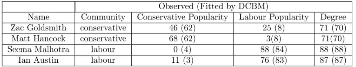
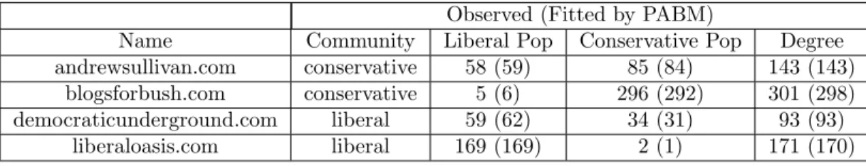
3.1 Illustrative nodes for political blogs, with popularities fit by DCBM

inside parantheses. . . 34 3.2 Illustrative nodes for British MPs. Identities were looked up using

tweeterid.com. . . 34 3.3 Community detection error rates (number of misclustered

nodes in brackets) . . . 53 3.4 Goodness of fit measures for node popularity . . . 53 3.5 Illustrative nodes for political blogs (regularized EP). . . 53 3.6 Illustrative nodes for British MPs. Identities of the nodes of this

network were looked up using tweeterid.com. Abbreviations: Comm

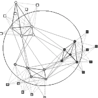
= community. . . 53 4.1 Top panel: the normalized MSEs for the bootstrap variance

esti-mators of nvar[median(x1,· · · , xn)] using (a) The grid based block

bootstrap (b) The dependent random weighting. The box for each row indicates the smallest normalized MSE among ln = 1,· · ·,10.

Bottom panel: the empirical coverage (in percent) for the bootstrap-based confidence intervals of the median using (a) and (b). The box for each row indicates the best coverage amongln = 1,· · ·,10

(Nom-inal level is 95%). . . 77 4.2 Top panel: the normalized MSEs for the bootstrap variance

estima-tors of nvar(¯xn) using (a) The dependent wild bootstrap (b) The

dependent random weighting (c) The grid based block bootstrap. The box for each row indicates the smallest normalized MSE among l= 1,· · ·,10. Bottom panel: the empirical coverage (in percent) for the bootstrap-based confidence intervals of the mean using (a), (b) and (c). The box for each row indicates the best coverage among

(10)

4.3 Top panel: the normalized MSEs for the bootstrap variance estima-tors of nvar(median(X1,· · · , Xn)) using (a) The grid based block

bootstrap (b) The dependent random weighting . The box for each row indicates the smallest normalized MSE among l = 1,· · ·,10. Bottom panel: the empirical coverage (in percent) for the bootstrap-based confidence intervals of the median using (a) and (b). The box for each row indicates the best coverage amongln = 1,· · ·,10

(Nom-inal level is 95%). 2D-case: n= 200,400, λn = 18,36 and ρ= 1 is

fixed. . . 79 4.4 Top panel: the normalized MSEs for the bootstrap variance

estima-tors of nvar(¯xn) using (a) The dependent wild bootstrap (b) The

dependent random weighting (c) The grid based block bootstrap. The box for each row indicates the smallest normalized MSE among l= 1,· · ·,10. Bottom panel: the empirical coverage (in percent) for the bootstrap-based confidence intervals of the mean using (a), (b) and (c). The box for each row indicates the best coverage among ln = 1,· · · ,10 (Nominal level is 95%). 2D-case: n = 200,400,

λn= 18,36 andρ= 1 is fixed. . . 80

5.1 Estimation time for different resampling methods . . . 88 6.1 Results for b=n0.8 _{after full run . . . 127}

6.2 Results for b =n0.7 after full run, with same (S,R) values

as in Table 2 . . . 128 6.3 Results for b=n0.7 _{after full run . . . 128}

(11)

LIST OF FIGURES

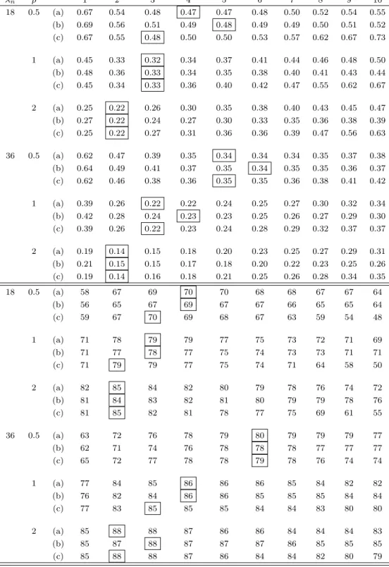
2.1 Sample heterogeneous network withT = 2, K = 3 andN = 30, with 5 type 1 nodes (circles) and 5 type 2 nodes (squares) in each block. Solid lines (black for intra-block, gray for inter-block) represent type 1-type 1 links, while dotted gray lines represent type 1-type 2 links. The homogeneous type

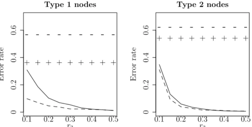
1-type 1 subnetwork is approximately enclosed in the circle. . 12 2.2 For simulation 1, Hom-SC errors are represented as ‘-’ forr1=r2=

0.1 and ‘+’ forr1 =r2 = 0.15, while Het-SC errors are represented by solid lines forr1 =r2= 0.1 and dashed lines for r1 =r2 = 0.15. For simulations 2 and 3, Hom-SC errors are represented as ‘-’ for r1 = 0.1 and ‘+’ forr1 = 0.15, while Het-SC errors are represented

by solid lines forr1= 0.1, and dashed lines forr1= 0.15. . . 24 2.3 For simulation 1, Hom-RSC errors are represented as ‘-’ forr1=r2=

0.1 and ‘+’ forr1=r2= 0.15, while Het-RSC errors are represented by solid lines forr1 =r2= 0.1 and dashed lines for r1 =r2 = 0.15. For simulations 2 and 3,r2= 0, and Hom-RSC errors are represented as ‘-’ for r1 = 0.1 and ‘+’ for r1 = 0.15, while Het-RSC errors are

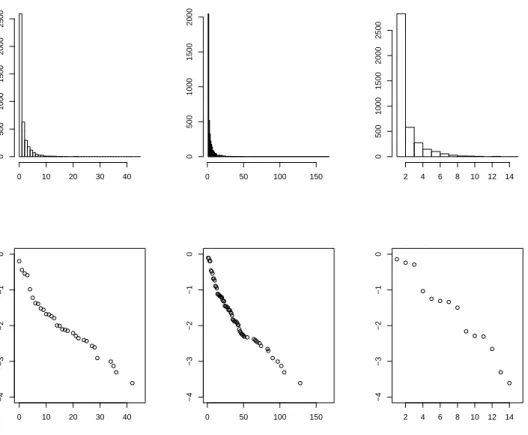
represented by solid lines forr1= 0.1, and dashed lines forr1= 0.15. . 25 2.4 DBLP author degree distribution of homogeneous author

collaboration network (left column), heterogeneous author-paper-conference network (middle column), and hetero-geneous author-conference network (right column). His-tograms (top row) of author node degrees have high fre-quency of low degrees, indicating that the author nodes are sparsely connected. The bottom row shows that the log empirical tail distributions log₁₀(1−Fˆ(x)) are roughly linear, suggesting power-law behavior of author node

(12)

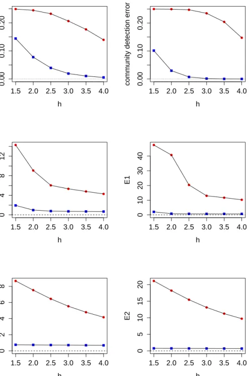
3.1 Community detection error and popularity estimation error plots from simulation study, where squares represent PABM errors and dots represent DCBM errors. The top row displays community de-tection errors measured byξnfrom (3.11), and the middle and bottom

rows display estimation errorsE1andE2from (3.13) and (3.14). We use sample sizes n = 400 (left) and n = 1000 (right). Homophily factor is increased fromh= 1.5 to h= 4 in increments of 0.5. The PABM modularity performs accurate community detection and

pop-ularity estimation, whereas results from DCBM are substantially poorer. 51 5.1 Time evolution of error rates for multiple linear regression

with d=100 (left column) and multiple logistic regression with d=10 (right column). Sample size n=100000, subset size is b = nγ _where _γ _{= 0}_._{6 (top row),} _γ _{= 0}_._{7 (middle}

row) and γ = 0.8 (bottom row). Bootstrap errors are rep-resented by solid lines, BLB errors by dashed lines, and SDB errors by dotted lines. Errors are averaged over 20

simulations. . . 95 5.2 AR(1) simulation results with_√ ξ = 95% quantile of Tn =

n(Mn−M), sample size n=100000, block length L=50,

autocorrelation ρ = -0.8 (top row), 0.5 (middle row), 0.9 (bottom row), and subset sizeb = 5000 (left column) ,10000 (right column). The plot displays the time evolution of error rates from 20 simulations when each method was al-lowed to run for 120 seconds. MBB errors are in solid lines,

BLB in dashed lines, and SDB in dottted lines. . . 102 5.3 AR(1) simulation results with_√ ξ = 5% quantile of Tn =

BLB in dashed lines, and SDB in dottted lines. . . 103 5.4 Time series regression simulation results with ξ = 95%

quantile of Tn =M SM/M SE, sample size n=100000,

di-mension d = 10, block length L=50, autocorrelation ρ = -0.8 (top row), 0.5 (middle row), 0.9 (bottom row), and subset size b = 5000 (left column) ,10000 (right column). The plot displays the time evolution of error rates from 20 simulations when each method was allowed to run for 60 seconds. MBB errors are in solid lines, BLB in dashed

(13)

5.5 Time evolution of ˆξfor CET dataset (measured in Celsius), whereξ = (q0.95−q0.05) is the width of the 90% confidence

interval forµbased onTn =

√

n( ¯X−µ). MBB was allowed to run for 600 seconds and BLB, SDB for 300 seconds. Block lengthL=50 (top row), 20 (middle row), 10 (bottom row), and subset size b= 5000 (left column) ,10000 (right column). MBB estimates are in solid lines, BLB in dashed

lines, and SDB in dottted lines. . . 105 5.6 AR(1) simulation results with_√ ξ = 95% quantile of Tn =

(14)

5.10 Time series regression simulation results with ξ = 95% quantile of Tn =M SM/M SE, sample size n=100000,

di-mension d = 10, block length L=10, autocorrelation ρ = -0.8 (top row), 0.5 (middle row), 0.9 (bottom row), and subset size b = 5000 (left column), 10000 (right column). The plot displays the time evolution of error rates from 20 simulations when each method was allowed to run for 150 seconds. MBB errors are in solid lines, BLB in dashed

lines, and SDB in dottted lines. . . 122 5.11 Time series regression simulation results with ξ = 95%

quantile of Tn =M SM/M SE, sample size n=100000,

di-mension d = 10, block length L=20, autocorrelation ρ = -0.8 (top row), 0.5 (middle row), 0.9 (bottom row), and subset size b = 5000 (left column), 10000 (right column). The plot displays the time evolution of error rates from 20 simulations when each method was allowed to run for 90 seconds. MBB errors are in solid lines, BLB in dashed

lines, and SDB in dottted lines. . . 123 6.1 Time evolution of error rates for multiple linear regression withd=100,

averaged over 50 simulations. Sample size n = 105_{, subset size is} b = n0.7 _{(top, middle),} _b ₌ _n0.8 _{(bottom). Bootstrap errors are in} solid red, SDB in solid blue, BLB in solid black, and ALB errors in dotted black. Forb =n0.7_{, we have} _S(R_{+ 1) = 500 in the top row,} S(R+ 1) = 200 in the middle row. For clarity we have only plotted

S= 1,2,3,4,5 for b=n0.7in the top row. . . 129 6.2 Time evolution of error rates. The red bar is the Normal

Approximation error, while the errors from residual boot-strap are in solid lines and errors from SRB are in dashed

(15)

CHAPTER 1 INTRODUCTION

1.1 Statistical analysis of networks with community

structure

Many complex systems in today’s world consist, at an abstract level, ofagents

whointeract with one another. This general agent-interaction framework de-scribes many interesting and important systems, such as social interpersonal systems (Milgram, 1967), protein interaction systems (Gavin et al., 2002), power grids (Watts and Strogatz, 1998), and the World Wide Web (Huber-man and Adamic, 1999), to name a few. Networks provide a convenient and unified way of representing such systems arising from diverse applications. It is therefore important to develop methodology for network data, and accord-ingly, the science of network data has received attention from scientists in various academic fields. A holistic introduction to the interdisciplinary study of networks can be found in Newman (2010). Statistically oriented overview of networks can be found in Goldenberg et al. (2010) and Kolaczyk (2009).

The early approach to network modeling, the random graph model by Erd¨os and R´enyi (1959), assumed that all agents behave in identical fash-ion. The observed dissimilarity in agent behavior was assigned to random fluctuations. This explanation might not always be appropriate, particularly when the network displays structured dissimilarities in agent behavior. At the other end of the modeling spectrum, one might wish to capture the ob-served variation in agent behavior by assigning a separate model to each individual agent. However, this might be impractical for networks beyond a certain size, and also unnecessary.

Real world networks often exhibit apatterned dissimilarity that lies some-where between completely identical agent behavior and completely unequal agent behavior. The agents are often found to cluster into groups or

(16)

commu-nities that display similar behavior, while agents from different commucommu-nities behave differently. The identification of this network structure, called com-munity detection, is an important problem in network analysis. Community detection has important real-world interpretation; these communities often turn out to be groups of agents which share common properties and/or play similar roles within the network. For example, in Jonsson et al. (2006), the communities in a protein interaction network turned out to be functional groups (proteins having the same or similar function) — this conclusion has important implications for cancer research. Fortunato (2010) provides a mul-tidisciplinary exposition on community detection in networks.

In Chapter 2, we consider heterogeneous networks which seems to have not been considered in the statistical community detection literaure. Many real-world systems consist of severaltypes of entities, and heterogeneous networks are required to represent such systems. However, the current statistical tool-box for network data can only deal with homogeneous networks, where all nodes are supposed to be of the same type. This article introduces a sta-tistical framework for community detection in heterogeneous networks. For modeling heterogeneous networks, we propose heterogeneous versions of both the classical stochastic blockmodel and the degree-corrected blockmodel. For community detection, we formulate heterogeneous versions of standard spec-tral clustering and regularized specspec-tral clustering. We also demonstrate the theoretical accuracy of the proposed heterogeneous methods for networks generated from the proposed heterogeneous models. Our simulations estab-lish the superiority of proposed heterogeneous methods over existing homoge-neous methods in finite networks generated from the models. An analysis of the DBLP four-area data demonstrates the improved accuracy of the hetero-geneous method over the homohetero-geneous method in identifying research areas for authors.

In ongoing work in Chapter 3, we consider the problem of modeling of popularity of nodes across communities, which is network feature closely as-sociated with community structure. In this chapter we introduce a new ran-dom graph model, called popularity-adjusted blockmodel (PABM, hereafter) for networks with community structure. Our model incorporates popularity parameters for each node that can take different values for different commu-nities. The profile likelihood for this model is formulated as a modularity function for community detection. We compare the methodology with

(17)

exist-ing methodology usexist-ing simulated and real networks.

1.2 Bootstrap methods for big data

Given a dataset, the primary task of data analysis is usually to perform some kind of statistical inference on this data. This inference task can be the es-timation of a parameter of interest, the test of a statistical hypothesis, and so on. A secondary task that is inextricably associated with any statistical inference method, is to assess the risk or precision associated with that in-ference. For example, suppose the goal of data analysis is the estimation of the population mean, and this primary task of estimation is performed using the sample mean. A natural next step would be the task of evaluating the degree of precision of the sample mean as an estimator of the population.

A measure of the precision of an inference method usually refers to the un-known sampling distribution of a statistic, the underlying distribution from which the observed sample mean can be visualized as a random draw. Often we have theoretical ideas about the sampling distributions in an asymptotic sense, but very little empirical information, since all we observe is a single random draw from this distribution. If it was possible to repeatedly draw random samples from this unknown distribution, we could have more empir-ical information on it. However, this is typempir-ically not feasible in practice. An approximate computational method is resample — consider the sample as a proxy for the population, and draw repeated resamples from the sample. Resampling methods provide a general and powerful method of evaluating the precision of a wide variety of statistical inference methods.

In chapter 4, we consider the problem of resampling for irregularly spaced dependent data. Traditional block-based resampling or subsampling schemes for stationary data are difficult to implement when the data are irregularly spaced, as it takes careful programming effort to partition the sampling re-gion into complete and incomplete blocks. We propose a new resampling method, the dependent random weighting, for both time series and random fields. The method is a generalization of the traditional random weighting in that the weights are made to be temporally or spatially dependent and are adaptive to the configuration of the data. Unlike the block-based bootstrap or subsampling methods, the dependent random weighting can be used for

(18)

irregularly spaced time series and spatial data without any implementational difficulty. Consistency of the distribution approximation is shown for both equally and unequally spaced time series. Simulation studies illustrate the finite sample performance of the dependent random weighting in comparison with the existing counterparts for both one dimensional and two dimensional irregularly spaced data.

In chapter 5, we consider the problem of resampling in massive data. The bootstrap is a popular and powerful method for estimating precision of es-timators and inferential methods. However, for massive datasets which are increasingly prevalent, the bootstrap becomes prohibitively costly in compu-tation and its feasibility is questionable even with modern parallel computing platforms. Recently Kleiner et al. (2014) proposed a method called BLB (Bag of Little Bootstraps) for massive data which is more computationally scalable with little sacrifice of statistical accuracy. Building on BLB and the idea of fast double bootstrap, we propose a new resampling method, the subsampled double bootstrap, for both independent data and time series data. In theory, we establish the consistency of our subsampled double bootstrap under mild conditions for both independent and dependent cases. Methodologically, the subsampled double bootstrap is superior to BLB in terms of running time, more sample coverage and automatic implementation with less tuning param-eters for a given time budget. Its advantage relative to BLB and bootstrap is also demonstrated in numerical experiments and data illustrations.

In chapter 6, we continue studying bootstrap methods for big data appli-cations. Extending the underlying idea of scaling down the effective sample size, we introduce two new resampling strategies for big data. The first strat-egy is called aggregation of little bootstraps or ALB, a generalized resampling technique that includes the SDB as a special case. Instead of taking the mean of estimates from different subsets (as in BLB), we aggregate all resampled roots{T∗∗,s,r

n }s=1,...,S,r=1,...,Rinto a single ensemble, and compute the precision

measure from the empirical cdf of this ensemble. The second strategy is called subsampled residual bootstrap or SRB, a fast version of residual bootstrap intended for massive regression models. Instead of a full-size resampling of regression residuals, we construct a subsample and use appropriate scaling adjustments to obtain a fast alternative to classical residual bootstrap. We study both methods through simulations.

(19)

CHAPTER 2 SPECTRAL CLUSTERING IN

HETEROGENEOUS NETWORKS

2.1 Introduction

Many complex systems in today’s world consist, at an abstract level, of agents

whointeract with one another. This general agent-interaction framework describes

many interesting and important systems, such as social interpersonal systems (Mil-gram, 1967), protein interaction systems (Gavin et al., 2002), power grids (Watts and Strogatz, 1998), and the World Wide Web (Huberman and Adamic, 1999), to name a few. Networks provide a convenient and unified way of representing such systems arising from diverse applications. It is therefore important to develop methodology for network data, and accordingly, the science of network data has received attention from scientists in various academic fields. A holistic introduc-tion to the interdisciplinary study of networks can be found in Newman (2010). Statistically oriented overview of networks can be found in Goldenberg et al. (2010) and Kolaczyk (2009).

The early approach to network modeling, the random graph model by Erd¨os and R´enyi (1959), assumed that all agents behave in identical fashion. The observed dissimilarity in agent behavior was assigned to random fluctuations. This expla-nation might not always be appropriate, particularly when the network displays structured dissimilarities in agent behavior. At the other end of the modeling spectrum, one might wish to capture the observed variation in agent behavior by assigning a separate model to each individual agent. However, this might be impractical for networks beyond a certain size, and also unnecessary.

Real world networks often exhibit apatterned dissimilarity that lies somewhere between completely identical agent behavior and completely unequal agent behav-ior. The agents are often found to cluster into groups or communities that display similar behavior, while agents from different communities behave differently. The identification of this network structure, called community detection, is an impor-tant problem in network analysis. Community detection has imporimpor-tant real-world

(20)

interpretation; these communities often turn out to be groups of agents which share common properties and/or play similar roles within the network. For example, in Jonsson et al. (2006), the communities in a protein interaction network turned out to be functional groups (proteins having the same or similar function) — this con-clusion has important implications for cancer research. Fortunato (2010) provides a multidisciplinary exposition on community detection in networks.

The currently available methodologies for network data usually consider net-works to be homogeneous, that is, the nodes in the network represent objects of the same type and all links in the network represent the same type of relation. For example, a friendship network, say Facebook, has nodes representing persons or users, and links representing friendship between users. However, many real-world systems are actually heterogeneous, in the sense that there are different types of agents, and various kinds of interactions in the system. Consequently, networks representing such systems are also heterogeneous, where several types of nodes and several types of links exist in the same network. Typically, for each node or link it is known what the type is, and a heterogeneous network contains this type infor-mation. For example, in Facebook, nodes can represent various types of entities like users, events, groups, celebrity pages, photos, and so on. Accordingly, there can be various types of links: friendship link between two users, membership link between users and groups, fan (or like) link between users and celebrities, atten-dance link between users and events, tag link between a photo and an user, and so on. The homogeneous ‘friendship network’ representation, that was mentioned earlier, effectively represents only a sub-system of this system, consisting only of ‘user’ nodes and ‘friendship’ links.

To analyze a heterogeneous network using the current toolbox of homogeneous methods and homogeneous models, there are two options — either consider a ho-mogeneous sub-network of the original network, or treat the heterogeneous network as a homogeneous network, suppressing the type information available in the data. In the first approach, there is loss of useful information. In the second approach the results might be meaningless as nodes of different types are grouped into the same community, or the procedure might not work well due to the presence of different types of nodes.

For example, consider a heterogeneous Facebook network consisting of two types of nodes — users and events, and two kinds of links: user-user or friendship links, and user-event orattendance links. Suppose network data in this form is available for users and events corresponding to 10 universities, and the problem of interest is to assign users to their universities using a clustering procedure. Using the

(21)

first option, one must carry out the analysis based on the user-user network only, dumping the event nodes and user-event links. In this context the dumped data can be quite important in predicting university affiliation. Using the second option, one treats the entire network as a homogeneous network and carries out a clustering of both users and events. However, users and events behave in very different ways, and the clustering algorithm might not work well since it is trying to cluster these different entities into the same clusters by comparing their behavior. Using K -means intuition, the ‘distance’ between an user and an event, both affiliated to the same university, might be too large.

Thus, community detection in heterogeneous network data cannot be satisfacto-rily carried out by applying homogeneous models and methodologies. A preferable approach is to have a procedure that uses the entire heterogeneous information, identifies the fact that users and events are different types of entities, and clusters nodes from different types separately but simultaneously into 10 user clusters and 10 event clusters. Since this procedure compares events to events and users to users, the clustering should work much better.

Heterogeneous networks have begun to receive attention from various scien-tific communities, particularly the computer science research community (Sun and Han, 2012). This chapter provides a statistical framework to deal with hetero-geneous network data by extending the existing homohetero-geneous framework. For modeling heterogeneous networks, we propose heterogeneous versions of the clas-sical stochastic blockmodel and the degree-corrected blockmodel recently proposed by Karrer and Newman (2011). For community detection in heterogeneous net-works, we formulate heterogeneous versions of standard spectral clustering and regularized spectral clustering. We also demonstrate the theoretical accuracy of the proposed heterogeneous methods for networks generated from the proposed heterogeneous models in the asymptotic framework of Qin and Rohe (2013).

As a real-world application of our methods, we implement our algorithm on a large bibliographical network from DBLP with the objective of identifying re-search area of authors. Under the existing homogeneous paradigm, the natural choice of network would be the co-authorship network with authors as nodes. We find that homogeneous clustering applied on the co-authorship network performs rather poorly, with an accuracy comparable to random assignment. However, in-terpreting the bibliographical network as a heterogeneous network (with authors, papers and conferences treated as different types of nodes), the heterogeneous clustering method performs quite accurate community detection.

(22)

theoretical notation that is used throughout the chapter. Section 2.3 reviews ex-isting homogeneous blockmodels and introduces heterogeneous versions of these models. Section 2.4 discusses the standard and regularized spectral clustering al-gorithms and presents modified versions of these alal-gorithms that are appropriate for heterogeneous networks. Section 2.5 provides a brief outline of the asymptotic framework of Qin and Rohe (2013), and demonstrates the asymptotic accuracy of the heterogeneous algorithms under the heterogeneous models, using this frame-work. Section 2.6 presents simulation studies demonstrating various circumstances under which the heterogeneous methods can provide significant improvements in clustering accuracy over the homogeneous methods. Section 2.7 presents a real-life example of the superiority of the heterogeneous method over the homogeneous method, using the DBLP four-area dataset. The chapter concludes with the dis-cussion in Section 3.7.

2.2 Graph Theoretic Notation

Mathematically a network is represented as a graph G= (V, E) consisting of two types of elements, namelynodes (orvertices) that comprise the setV, andlinks(or

edges) that make up the set E. Every link has two endpoints in the set of nodes,

and is said toconnect orjoin the two nodes. The two endpoints of a link are also said to be adjacent to each other, orneighbors. An unweighted, undirected graph containing no self-loops or multiple edges is called a simple graph. Thedegree dv

of a node v in a graphG is the number of nodes adjacent tov. A degree sequence

is a list of degrees of a graph in non-increasing order (e.g., d1 ≥d2≥ · · · ≥dn).

An adjacency matrix A is often used to represent a graph: for a graph with

N nodes, it is an N-by-N matrix whose (i, j)-th entry gives the number of links from thei-th node to the j-th node. This chapter covers simple graphs only, and hence the adjacency matrix is symmetric, consists only of 0’s and 1’s, and all its diagonal entries are zero.

The Graph Laplacian L is a matrix frequently used in network analysis. There

are several ways of defining the Laplacian; in this chapter it is defined as

L=D−12AD− 1

2, (2.1)

whereAis the adjacency matrix andDis the degree matrix (i.e., a diagonal matrix whoseith _{diagonal element is the degree of node} _i_{). This version of the Laplacian}

(23)

is often referred to as the symmetric normalised Laplacian, but this chapter will simply refer to this as the Laplacian.

2.3 Stochastic Blockmodel and Degree Corrected

Blockmodel for Heterogeneous Networks

Lorrain and White (1971) were the first to introduce blockmodels, in association with the deterministic concept of structural equivalence, where two nodes of a network are considered equivalent if they have the same set of neighbors. Holland et al. (1983) and Fienberg et al. (1985) generalized this equivalence concept to a probabilistic setting, calling it stochastic equivalence. In contrast to structural equivalence which is defined with respect to the observed network itself, stochastic equivalence is defined with respect to the conceptual model that generates the observed network.

Definition Two nodes in a network are said to be stochastically equivalent if the probability of any event pertaining to the network remains unchanged by exchanging the node labels.

For a homogeneous network, two nodes (say, 1 and 2) are stochastically equiv-alent according to this definition if they have the same probability of being linked toany third node (say 3).

2.3.1 Homogeneous model

Consider a simple graph G = (V, E) with N nodes, and let A be its adjacency matrix. Note that A is a symmetric 0-1 matrix, and its diagonal entries are all zero. Under the K-block stochastic blockmodel, there are K blocks, and each node belongs to one of these blocks. LetMdenote theN-by-K block membership matrix with M(i, k) = 1 if node iis in the kth block, andM(i, k) = 0 otherwise. Then for i < j, under the stochastic blockmodel (SBM) A(i, j) are Bernoulli random variables, with

E[A(i, j)|M] =M(i,·)PM(j,·)0, (2.2)

wherePis theK-by-K matrix of link probabilities, that is,P(a, b) represents the probability that a node in block ais linked to another node in blockb. Edges are conditionally independent given the membership matrix M.

(24)

Model (3.2) essentially means that if nodesi andi0 come from the same block, i.e., M(i,·) = M(i0,·), then they are stochastically equivalent; for anyj different from iand i0, the linksA(i, j) andA(i0, j) are exchangeable — hence, exchanging the node labels of iand i0 will make no difference to the probability of any event in the network.

Stochastic equivalence theorizes that two nodes in the same block have identical degree distributions. This can be an unrealistic assumption for many empirical networks. The degree-corrected blockmodel (DCBM) proposed by Karrer and Newman (2011) adds degree scaling parameters θi for each node to allow for a

broad degree distribution. Then for i < j, under the DCBMA(i, j) are Bernoulli random variables, with

E[A(i, j)|M] =Θ(i,·)MPM0Θ(·, j) (2.3)

whereΘis anN-by-N diagonal matrix withΘ(i, i) =θi, the degree parameter of

theith node, and all other parameters have the same meaning as (3.2).

Note that the SBM is a special case of the DCBM when all nodes in the same block have equal value of theθi, the degree parameter.

2.3.2 Heterogeneous model

A heterogeneous network has nodes of several different types. Nodes of different types are fundamentally different in their role in the network. Similarly, the links in the network are also of different kinds, depending upon the types of the nodes they link. Therefore, a blockmodel for heterogeneous networks should allow the link probabilities to change not only by block but also by node type. We propose the following model for accommodating this.

Consider a K-block heterogeneous network withN nodes of T different types. We divide each block intoT sub-blocks for different types of nodes such that each type-block combination is represented by a separate sub-block. Let M represent

theN-by-T Ksub-block membership matrix, withM(i, t×k) = 1 if nodeiis of the

tthtype and belongs to thekthblock, andM(i, t×k) = 0 otherwise, fort= 1, . . . , T and k= 1, . . . , K. Let P be theT K-by-T K matrix of link probabilities. ThenP has the following structure:

(25)

P=       P11 P12 . . . P1T P21 P22 . . . P2T . . . PT1 PT2 . . . PT T       ,

where Pst is the K-by-K matrix of probabilities for type s-type t links. Thus, Pst(a, b) represents the probability that a node of the sth type and belonging to

blocka is linked to another node of thetth type and belonging to block b. As before, for i < j,A(i, j) are Bernoulli random variables, with

E[A(i, j)|M] =M(i,·)PM(j,·)0 (2.4)

for the heterogeneous stochastic blockmodel (Het-SBM) and

E[A(i, j)|M] =Θ(i,·)MPM0Θ(·, j) (2.5)

for the heterogeneous degree-corrected blockmodel (Het-DCBM).

This complicated representation of link probabilities is necessary, because link probabilities vary not only by block, but also by type; Pst(a, b) varies not only

with aandb but also withsand t.

For illustration, consider a toy example for Het-SBM with number of types T = 2, the number of blocks K = 3 and the number of nodes N = 30, with 5 type 1 nodes and 5 type 2 nodes in each block, and the link probability matrix as follows: P=               0.75 0.25 0.25 0.90 0.00 0.00 0.25 0.75 0.25 0.00 0.90 0.00 0.25 0.25 0.75 0.00 0.00 0.90 0.90 0.00 0.00 0.00 0.00 0.00 0.00 0.90 0.00 0.00 0.00 0.00 0.00 0.00 0.90 0.00 0.00 0.00               .

Link probabilities vary prominently across blocks as well as types in this model. Type 1 nodes are strongly homophilic (intra-community links are much more likely than inter-community links), while type 2 nodes are not linked among themselves at all. The type 1-type 2 links have even stronger homophily; type 1 and type 2 nodes belonging to the same block are very likely to be connected, while inter-block, inter-type links are not present. This model is an exaggerated representation of the user-event heterogeneous Facebook system mentioned in the introduction.

(26)

In Figure 2.1, type 1 nodes and type 2 nodes are clearly different in their roles in the network, nevertheless they form close-knit communities. Visually, it appears that community structure is stronger in the entire network, compared to the ho-mogeneous type 1-type 1 subnetwork. This toy example gives a visual intuition of how community discovery might be more accurate in the presence of heterogeneous information.

Figure 2.1: Sample heterogeneous network with T = 2, K = 3 and N = 30, with 5 type 1 nodes (circles) and 5 type 2 nodes (squares) in each block. Solid lines (black for intra-block, gray for inter-block) represent type 1-type 1 links, while dotted gray lines represent type 1-type 2 links. The

homogeneous type 1-type 1 subnetwork is approximately enclosed in the circle.

2.4 Spectral Clustering and Regularized Spectral

Clustering

2.4.1 Homogeneous clustering

Consider a homogeneous network withN nodes and letAbe its adjacency matrix. Assuming a correctly specifiedK-block blockmodel structure for this network, the

(27)

standard spectral clustering algorithm assigns the N nodes to K clusters in the following steps.

Homogeneous Spectral Clustering Algorithm (Hom-SC)

1. Given the adjacency matrixA, calculate the graph Laplacian L by (2.1). 2. Find orthonormal eigenvectors X1, . . . ,XK corresponding to the K

eigen-values of L that are largest in absolute value. Put them into theN-by-K matrix X= [X1, . . . ,XK].

3. Carry out a K-means clustering with the N rows of matrix X, creating a K-partition of the index set{1, . . . , N}.

4. Assign the nodes to clusters in accordance to the clustering obtained in step 3, i.e., assign the ith node to thekth cluster if the ith row got assigned to thekth cluster in step 3.

Recent work by Amini et al. (2013) and Jin (2012) demonstrate that homoge-neous spectral clustering does not work very well in sparse homogehomoge-neous networks with wide degree distribution. Chaudhuri et al. (2012) proposed a regularized version of the graph Laplacian for sparse networks and it was shown by Qin and Rohe (2013) that a normalized variant of spectral clustering on this regularized Laplacian has superior theoretical properties under the degree corrected stochastic blockmodel. In this context we would also like to mention Joseph and Yu (2013) for their in-depth analysis of the performance of a slightly different version of regularized spectral clustering.

For a regularizerτ ≥0, define the regularized degree matrixDτ =D+τI and

the regularized graph Laplacian

Lτ =Dτ−1/2AD−τ1/2. (2.6)

Following the recommendation of Qin and Rohe (2013), in this paper we set τ equal to the average node degree of the network, in all applications of regularized spectral clustering (homogeneous and heterogeneous) for simulations as well as data analysis. The regularized spectral clustering algorithm assigns the N nodes toK clusters in the following steps.

Homogeneous Regularized Spectral Clustering Algorithm (Hom-RSC) 1. Given the adjacency matrix A and regularizer τ ≥ 0, calculate regularized graph LaplacianLτ by (2.6).

2. Find orthonormal eigenvectorsX1, . . . ,XK corresponding to theK

(28)

Xτ = [X1, . . . ,XK].

3. Normalize each row of Xτ to have unit norm, forming the N-by-K matrix X∗_τ given byX∗_τ(i, j) =Xτ(i, j)

.q P

jXτ(i, j)2.

4. Carry out a K-means clustering with the rows of matrix X∗_τ, creating a K-partition of the index set{1, . . . , N}.

5. Assign the nodes to clusters in accordance to the clustering obtained in step 4, i.e., assign the ith node to thekth cluster if the ith row got assigned to thekth cluster in step 4.

2.4.2 Heterogeneous clustering

For aT-type heterogeneous network, there areT Kclusters (since each type-block combination represents a cluster), but for each node, the type information is al-ready known. So essentially there are T cluster assignment problems — to assign then1 type 1 nodes intoK clusters, then2 type 2 nodes intoK separate clusters,

and so on. This can be achieved by carrying out T simultaneous but separate

K-means clustering procedures. We now present heterogeneous versions of the Hom-SC and Hom-RSC algorithms based on this idea.

Heterogeneous Spectral Clustering Algorithm (Het-SC)

1. Given the adjacency matrixA, calculate the graph Laplacian L by (2.1). 2. Find orthogonal eigenvectors X1, . . . ,XT K corresponding to the T K

eigen-values ofL that are largest in absolute value. Put them into theN-by-T Kmatrix X= [X1, . . . ,XT K].

3. For each t = 1, . . . , T, select the nt rows of X that correspond to nodes of

type t, and carry out separate K-means clustering for each selection, creating a T K-partition of the index set{1, . . . , N}.

4. Assign the nodes to clusters in accordance to the clustering obtained in step 3, i.e., assign the ith node to the rth cluster if the ith row got assigned to the rth cluster in step 3.

Heterogeneous Regularized Spectral Clustering Algorithm (Het-RSC) 1. Given the adjacency matrixAand regularizerτ ≥0, calculate the regularized graph LaplacianLτ by (2.6).

2. Find orthogonal eigenvectors X1, . . . ,XT K corresponding to the T K

eigen-values ofLτ that are largest in absolute value. Put them into theN-by-T Kmatrix Xτ = [X1, . . . ,XT K].

(29)

3. Normalize each row ofXτ to have unit norm, forming the N-by-T K matrix X∗_τ given byX∗_τ(i, j) =Xτ(i, j)

.q P

jXτ(i, j)2.

4. For eacht = 1, . . . , T, select the nt rows ofX∗τ that correspond to nodes of

type t, and carry out separate K-means clustering for each selection, creating a T K-partition of the index set{1, . . . , N}.

5. Assign the nodes to clusters in accordance to the clustering obtained in step 4, i.e., assign the ith node to the rth cluster if the ith row got assigned to the rth cluster in step 4.

In the next section we provide theoretical justification of why the Het-RSC algorithm works under the Het-DCBM model and the Het-SC algorithm works under the Het-SBM model.

2.5 Convergence of Heterogenous Spectral Clustering

This section outlines an asymptotic theory for the convergence of the Hom-RSC algorithm under the Hom-DCBM, and proposes a similar result for the Het-RSC algorithm under the Het-DCBM. Convergence of the Het-SC algorithm under the Het-SBM follows as a special case. The interested reader is directed to Qin and Rohe (2013) for technical details for the homogeneous case.

For the Hom-DCBM (3.3), define A = ΘMPM0Θ and let D be the diagonal matrix of expected degrees, i.e., D(i, i) =P

jA(i, j). DefineDτ =D+τI and let

L_τ =D−_τ1/2AD_τ−1/2 be the population version of the regularized graph Laplacian (2.6). Under a K-block Hom-DCBM, L_τ has exactly K non-zero eigenvalues. Let X_τ be the N-by-K matrix of the corresponding eigenvectors. Finally, X∗

τ is

the row-normalized version of X_τ. The main idea is to interpret the clustering algorithm as an estimation procedure for X∗ withX∗

τ as the parameter.

Let δ = mini=1,...,ND(i, i) be the minimum expected degree, and let λ be the

magnitude of the smallest non-zero eigenvalue of L_τ in magnitude. Let γ = mini=1,...,N{min{||Xτ(i,·)||2,||Xτ(i,·)||2} be the length of the shortest row in Xτ

andXτ, where||x||2 represents theL2 norm of the vectorx. Assume that for some

>0 and sufficiently largeN,

(A1)δ+τ >3 log(4N/) and (A2)λ≥8 r

3Klog(4N/) δ+τ .

(30)

Theorem 4.2 of Qin and Rohe (2013) states: when (A1) and (A2) hold, then ||Xτ − XτO||F ≤c0 1 λ r Klog(4N/) δ+τ (2.7) and ||X∗_τ− X_τ∗O||F ≤c0 1 γλ r Klog(4N/) δ+τ (2.8) for some constant c0 with probability at least 1−, where O represents an

or-thonormal rotation, and|| · ||F denotes the Frobenius norm of a matrix, defined as

||B||F = q P i P j|B(i, j)|2.

The next step is to translate this accuracy in estimation of X_τ∗ into accurate clustering of nodes. Lemma 3.3 of Qin and Rohe (2013) shows that X∗

τ can be

written as X∗

τ =MB, where B is a K-by-K non-singular matrix. Note that the

membership matrix M has exactly K unique rows. Hence, X∗

τ also has exactly

K unique rows. This implies that a K-means clustering applied on the rows of

X∗

τ would perfectly identify the block membership of all nodes in the network.

Given the asymptotic closeness between X∗_τ and X∗

τ from (2.8), one might expect

that the clustering output from X∗_τ also approaches the clustering output from

X∗

τ asymptotically. As discussed above, the clustering output from Xτ∗ is perfect;

hence, the clustering output fromX∗_τis expected to approach that perfect accuracy in an asymptotic sense.

To formalize this intuition, a mathematically tractable definition of miscluster-ing is required. In step 4 of the regularized spectral clustermiscluster-ing algorithm, the N rows of X∗_τ are subjected to a K-means clustering, which assigns each row to a cluster, and each cluster thus formed will have a centroid. Let Cbe the N-by-K matrix of cluster centroids, i.e., C(i,·) is the centroid corresponding to the ith row of X∗_τ. ThenX_τ∗(i,·) is the parameter centroid corresponding to the ithnode, while the estimated centroid is C(i,·). It is therefore reasonable to consider the ith node to be correctly clustered if the estimated centroid is closer to the correct parameter centroid than the remaining K−1 incorrect parameter centroids, and it is misclustered if the estimated centroid is closer to some incorrect parameter centroid than the correct parameter centroid.

Definition The set of misclustered nodesE is defined as

E={i:∃ j6=i s.t.||C(i,·)− X_τ∗(i,·)O||₂ >||C(i,·)− X_τ∗(j,·)O||₂}. (2.9)

(31)

hold. Then Theorem 4.4 of Qin and Rohe (2013) states that, with probability at least 1−,

|E| ≤c1

Klog(N/)

γ2_λ2₍_δ₊_τ₎ (2.10)

for some constantc1.

Next, we extend these ideas to the Het-DCBM and the Het-RSC algorithm. For theT-type, K-block Het-DCBM from Section 2.3.2,MhasT K unique rows, and P is T K-by-T K, since link probabilities are allowed to vary for each type-block combination. Note that this model is structurally equivalent to a Hom-DCBM (3.3) with T K blocks. The interpretation of sub-blocks in a T-type, K-block heterogeneous model is different from that of blocks in a T K-block homogeneous model, but both models have the same mathematical structure. Consequently, the convergence result for row-normalized eigenvectors in (2.8) can be directly applied to the heterogeneous model.

The translation of estimation accuracy to clustering accuracy, however, does not extend directly from the homogeneous version to the heterogeneous version. The upper bound in (2.10) for the homogeneous case is derived from the fact that the matrix of cluster centroids,C, is the minimizer of theK-means objective function

||X∗_τ −Y||_F, minimization being performed over the set of all N-by-K matrices Y having exactly K unique rows. The Het-RSC algorithm in Section 2.4.2 runs T separate K-means procedures on the T node types, thereby using a different objective function. Therefore, (2.10) does not apply directly to heterogeneous net-works. However, after considering the modified objective function being minimized in step 4 of the Het-RSC algorithm, we are able to prove the following theorem, which provides the heterogeneous version of (2.10).

Theorem 2.5.1 Consider a T-type, K-block Het-DCBM with nt nodes of type t,

and N =PT

t=1nt. For nodes of typet, define the set of misclustered nodes Et as

E_t={i∈type t:∃ j∈type t&j 6=i s.t.

||C(i,·)− X_τ∗(i,·)O||2 >||C(i,·)− Xτ∗(j,·)O||2}. (2.11)

Let γt= mini∈typet{min{||Xτ(i,·)||2,||Xτ(i,·)||2} be the length of the shortest row

of type t in Xτ andXτ, and λ, δ, τ be defined as before. For some >0 and

suffi-ciently large N, suppose Assumptions (A1)and (A2) hold. Then with probability

at least 1−, |Et| ≤c1 Klog(N/) γ2 tλ2(δ+τ) for t= 1, . . . , T, (2.12)

(32)

where c1 is some constant.

The proof of Theorem 1 is in the Appendix.

Remark 1Two main assumptions of Theorem 1 are (A1) and (A2). Assump-tion (A1) requires a lower bound on the smallest regularized expected degreeδ+τ. This emphasizes the importance of regularization, as it allows expected node de-grees to be low, as long as they are complemented by the regularizer. Assumption (A2) requires that the smallest non-zero eigenvalue of Lτ in magnitude does not

decay to zero too fast. The number of types,T, is arbitrary but fixed. The number of blocks, K, is allowed to increase with nt and N as long as Assumptions (A1)

and (A2) hold true — thus its allowable rate on increase depends on the large sample behavior of the quantities δ, τ,and λ.

Theorem 1 provides a separate bound for each node type. Under Assumptions (A1) and (A2), for a given type t and for sufficiently large N, the quantity on the right hand side of (2.12) is O(1/γ_t2). Therefore as nt → ∞, the asymptotic

bound on the number of misclustered nodes depends on the behavior ofγt. When

γt decays at a rate slower than p

1/nt, the bound in (2.12) implies that the error

rate |Et|/nt goes to zero. The bound deteriorates when γt decays to zero faster

thanp1/nt. Note that it is plausible that the bound goes to zero for certain node

types, but not for others — depending upon the behavior of γt for different node

types.

Remark 2 (Application to Het-SC under Het-SBM) The convergence of Hom-SC under Hom-SBM was first established by Rohe et al. (2011) under the assumptions of a dense network model. Their results can be extended from the homogeneous setting to the heterogeneous setting, but that would restrict the ap-plication to the dense network case. The framework of Qin and Rohe (2013) allows for sparse networks in a broader class of degree-corrected models, and although we have focussed on Het-RSC under Het-DCBM so far in this section, the results can be readily applied to Het-SC under Het-SBM as outlined below.

The main difference between the Het-SC algorithm and the Het-RSC algorithm is that the former does not have regularization or normalization steps. The Het-SBM is a special case of the Het-DCBM, when the degree parametersθi are equal.

In this special case, the model eigenvector matrix X_τ already has exactly T K distinct rows (applying Lemma 3.3 of Qin and Rohe (2013)) corresponding to the T K sub-blocks. Hence, row-normalization is not required — we can cluster the rows of Xτ directly and use the result in (2.7). Further, we can set the

(33)

regularization is lost, and the network model is required to satisfy the following restricted version of (A1) and (A2):

(A10)δ >3 log(4N/) and (A20)λ≥8 r

3Klog(4N/)

δ .

Hereλis the magnitude of the smallest non-zero eigenvalue ofL(the unregularized Laplacian) in magnitude. We obtain the following result for SC under the Het-SBM.

Theorem 2.5.2 Consider a T-type, K-block Het-SBM withnt nodes of typet, and

N =PT

t=1nt. LetCdenote the matrix of cluster centroids resulting from Het-SC,

and the set of misclustered nodes be defined as

Et={i∈type t:∃ j∈type t&j 6=i s.t.

||C(i,·)− X_τ₌₀(i,·)O||₂>||C(i,·)− X_τ₌₀(j,·)O||₂}. (2.13)

Let λ and δ be defined as before, and τ = 0. For some >0 and sufficiently large

N, suppose Assumptions(A10) and(A20) hold. Then with probability at least1−,

|Et| ≤c1

Klog(N/)

λ2₍_δ₊_τ₎ for t= 1, . . . , T, (2.14)

where c1 is some constant.

The proof for Theorem 2.5.2 is essentially similar to that for Theorem 2.5.1, the only difference being the use of the eigenvector matrix Xτ=0 instead of its

nor-malized version X_τ∗₌₀, and hence we skip the proof of Theorem 2.5.2 to avoid repetition.

2.6 Simulation Results

This section reports three simulation studies comparing the finite-sample perfor-mance of the homogeneous clustering algorithms with their heterogeneous coun-terparts in bi-type heterogeneous networks, i.e., T = 2. We study both Het-SBM and Het-DCBM in our simulation studies. Although Het-SBM is a special case of Het-DCBM, it is an important special case from a methodological perspective. Regularized spectral clustering adds two extra steps to standard spectral cluster-ing - regularization (step 1) and row-normalization (step 3). The former aims to

(34)

deal with sparsity (nodes with low expected degrees), while the latter aims to deal with non-uniformity in expected node degrees. In our simulations, both these fea-tures stem from degree parameters in Het-DCBM. For Het-SBM, the uniformity of expected node degrees makes both regularization and normalization unnecessary. Therefore, we study the performance of Het-SC vs Hom-SC under networks gen-erated from Het-SBM, and that of Het-RSC vs Hom-RSC in networks gengen-erated from Het-DCBM.

The class of Het-SBM models used for these simulations is B(K;s1, s2, p1, r1,

p2, r2, p3, r3) where K is the number of blocks, and s1 and s2 are the number of

type 1 and type 2 nodes per block, respectively. The probability matrix is given by P= P11 P12 P21 P22 ! ,where P11 = p11K10K+r1IK, P22 = p21K10K+r2IK, P12 = P21 = p31K10K+r3IK.

Here 1K is aK-vector of 1’s, and IK is theK-by-K identity matrix. Thus, in the

type 1-type 1 (type 2-type 2) homogeneous network, p1(p2) represents the

inter-block link probability while p1+r1 (p2 +r2) is the intra-block link probability.

The strength of homophily in the homogeneous networks is therefore determined by r1 and r2. For type 1-type 2 links, p3 represents the inter-block, inter-type

link probability and r3 represents the strength of inter-type homophily. For

Het-DCBM, we use the same values of P, K, s1,ands2. The degree parameters θi are

generated from the power law distribution

f(x) = β−1 xmin x xmin −β

withxmin = 1 and shape parameterβ= 3, and then scaled down so that the

aver-age ¯θ equals 1. For a given parameter combination, the Het-DCBM can therefore be interpreted as a ‘noisy’ version of the Het-SBM, or conversely the Het-SBM can be interpreted as an ‘averaged’ version of the Het-DCBM. For illustration, the model used in the example in Section 2.3.2 had K = 3, s1 = s2 = 5, p1 = 0.25,

r1= 0.50, p2 = r2 =p3 = 0, andr3 = 0.90.

Our main objective in these simulations is to study how the improved accuracy of heterogeneous clustering over homogeneous clustering depends on r3 for a fixed

(35)

more strongly homophilic, and therefore make heterogeneous community detection easier. Hence, we expect Het-SC and Het-RSC to be increasingly accurate with increasing r3, while Hom-SC and Hom-RSC are not affected byr3. However, the

actual improvement of heterogeneous clustering over homogeneous clustering will depend on other parameters as well, particularlyp1, r1, p2 and r2, which determine

the strength of homophily (and hence the ease of community detection) for the homogeneous networks.

To capture these dynamics, we fix K = 3, s1 = 100, s2 = 50, and p3 = 0.25.

Thus, we study networks having a total of N = 450 nodes, of which 300 are of type 1 and 150 are of type 2. The parameters p1, p2, r1, and r2 are set to various

combinations, to generate various kinds of homogeneous networks. For each such combination,r3is increased in a fixed grid, from 0.10 to 0.50 in increments of 0.05.

For each combination of parameters, error rates are estimated by averaging across 100 networks from Het-SBM and Het-DCBM.

It is important to note how clustering performance is measured in these simula-tions. Definitions (2.9), (2.11), and (2.13) introduced model-based quantification of misclustered nodes for the purpose of mathematical tractability, and the bounds (2.10), (2.12), and (2.14) were established under these definitions. However, these definitions require complete knowledge of the underlying model generating the net-work. For calculation of misclustering error in a real network, the true membership (ground truth) might be known (providing information about M), but the other model parameters will generally not be known, and hence these definitions can not be evaluated for real networks. Accordingly, the error rate used in these simula-tions is not the model-based quantity from Section 2.5, but rather it is the usual data-based error rate, defined below as the proportion of nodes that got assigned to wrong clusters.

For aK-block network model, thetruemembership (M) provides aK-partition, sayP, of the nodes. Suppose there are two competing clustering algorithms which also provide K-partitions, say P1 and P2 respectively. For each algorithm,

con-sider the K-by-K overlap table Ti such that Ti(k, l) is the number of nodes that

have been assigned to thekth _{block according to}_P_{and to the}_lth _{block according}

toP_i. ThenP

kTi(k, k) is the total number of correctly clustered nodes according

toP_i. However, due to potential identifiability issues with cluster labels,Ti should

not be used directly to compare the accuracy ofP₁ andP₂. For example, suppose P₁ gives the same partition asP, but with different cluster labels, whileP₂ is just a random partition. ThenP

kT1(k, k) = 0 and hencePkT2(k, k)>PkT1(k, k),

(36)

the columns of Ti to maximize PkTi(k, k). This is equivalent to relabeling the

clusters of Pi, and makes no change to the K-partition of the nodes. Now it is

reasonable to compare P1 and P2 on the basis of permutedT1 and T2. The

er-ror rate is defined as the sum of off-diagonal elements of Ti, divided by the total

number of nodes.

Thus, these simulations are not aimed at studying the finite-sample behavior of the quantities involved in the asymptotic theory, rather they are aimed at studying the relative accuracy of homogeneous and heterogeneous clustering methods in finite networks generated from Het-SBM and Het-DCBM.

2.6.1 Simulation 1

In this simulation we study homophilic networks where both types have similar inter-block and intra-block link probability. We use p1 = p2 = 0.25, and use

a single parameter, r1 = r2 = r, say, to govern the strength of homophily in

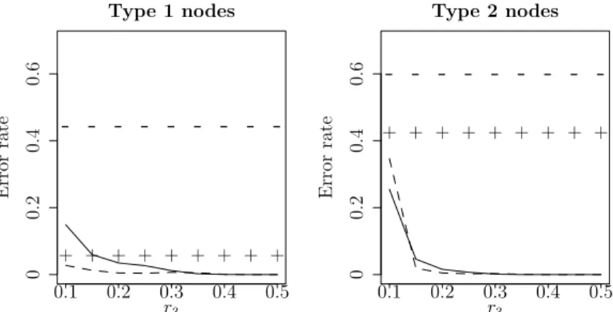
the homogeneous networks. Two values of r = 0.10,0.15 are used, to construct homogeneous networks of two different strengths. The error rates from Het-SBM and Het-DCBM are plotted in Figure 2.2(a) and Figure 2.3(a) respectively.

It is observed in both models that homogeneous error rates for type 1 nodes are substantially lower than type 2, implying the effect of sample size or block size on error rates. Homogeneous error rates also go down quite remarkably for both types asr is increased from 0.10 to 0.15, since the homogeneous network becomes more strongly homophilic, rendering community detection easier. This phenomenon is more prominent in Het-SBM (Figure 2.2(a)) than Het-DCBM (Figure 2.3(a)). However, the most striking observation in Figure 2.2(a) and Figure 2.3(a) is the improved accuracy of heterogeneous clustering over homogeneous clustering, for both types and both models. This comparative advantage increases with increasing r3, but it is significant even for smaller values of r3.

2.6.2 Simulation 2

A plausible scenario in heterogeneous networks is when the type 1-type 1 ho-mogeneous network is homophilic but the type 2-type 2 network does not have homophilic community structure. To model this, we use p1 = p2 = 0.25 as

be-fore, but set the type 2 homophily parameter r2 = 0 while the type 1 homophily

(37)

Figure 2.2(b) and Figure 2.3(b) show that the heterogeneous methods are much more accurate for both node types. The improved accuracy over the homogeneous method is particularly remarkable for type 2 nodes, because the homogeneous type 2-type 2 network does not have homophilic communities, and it would be quite difficult to assign communities to nodes on the basis of homogeneous information only. For example, consider a high school social network where students (type 1) form homophilic communities based on grades, but teachers (type 2) do not show homophily, rather they interact uniformly with other teachers. However, the heterogeneous student-teacher interaction is expected to be homophilic, as a student from a particular grade is expected to have more interaction with a teacher from the same grade, compared to a teacher from a different grade. In such a scenario, using a heterogeneous student-teacher network will most likely perform better community detection for both students and teachers, compared to clustering the homogeneous student-student network or the homogeneous teacher-teacher network, even though teacher-teachers do not interact in homophilic fashion.

2.6.3 Simulation 3

Another plausible situation is that type 1-type 1 interactions are homophilic but there is no type 2-type 2 interaction at all. We use p1 = 0.25 and increase r1

from 0.1 to 0.15 as before, but setp2=r2= 0, so that there are no links between

type 2 nodes. A motivation for this situation is the notional Facebook user-event heterogeneous network described in the introduction. While users (type 1) form a homophilic friendship network with universities as communities, there is no natural interaction between two events (type 2), implying a blank type 2-type 2 network. However, there is expected to be strong homophily in user-event interactions, and hence it is quite likely that the heterogeneous method will deliver a superior per-formance than the homogeneous method.

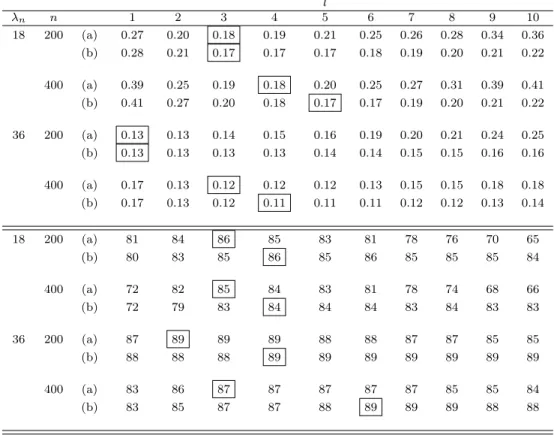
Figure 2.2(c) and Figure 2.3(c) show that the heterogeneous method is indeed significantly superior to the homogeneous method, for both types. In this case, it is theoretically impossible to implement homogeneous spectral clustering on the type 2-type 2 network, as the Laplacian for this network is a zero matrix, while the heterogeneous method delivers quite accurate clustering for type 2 nodes. For the sake of comparison, we have used a flat homogeneous error rate of 2/3 (random allocation with K= 3 clusters) for type 2 nodes.

(38)

0.1 0.2 0.3 0.4 0.5 0 0.2 0.4 0.6 Type 1 nodes r3 Error rate -+ -+ -+ -+ -+ -+ -+ -+ -+ 0.1 0.2 0.3 0.4 0.5 0 0.2 0.4 0.6 Type 2 nodes r3 Error rate -+ -+ -+ -+ -+ -+ -+ -+ -+

(a) Simulation 1: Both type 1-type 1 and type 2-type 2 networks are homophilic 0.1 0.2 0.3 0.4 0.5 0 0.2 0.4 0.6 Type 1 nodes r3 Error rate -+ -+ -+ -+ -+ -+ -+ -+ -+ 0.1 0.2 0.3 0.4 0.5 0 0.2 0.4 0.6 Type 2 nodes r3 Error rate -+ -+ -+ -+ -+ -+ -+ -+ -+

(b) Simulation 2: Type 1-type 1 networks have homophilic communities but type 2-type 2 networks do not have homophilic communities

0.1 0.2 0.3 0.4 0.5 0 0.2 0.4 0.6 Type 1 nodes r3 Error rate -+ -+ -+ -+ -+ -+ -+ -+ -+ 0.1 0.2 0.3 0.4 0.5 0 0.2 0.4 0.6 Type 2 nodes r3 Error rate -+ -+ -+ -+ -+ -+ -+ -+ -+

(c) Simulation 3: Homophilic type 1-type 1 networks and no type 2-type 2 links

Figure 2.2: For simulation 1, Hom-SC errors are represented as ‘-’ forr1=r2= 0.1 and ‘+’ forr1=r2= 0.15, while Het-SC errors are represented by solid lines for r1=r2= 0.1 and dashed lines forr1=r2= 0.15. For simulations 2 and 3, Hom-SC errors are represented as ‘-’ for r1= 0.1 and ‘+’ forr1= 0.15, while Het-SC errors are represented by solid lines forr1= 0.1, and dashed lines forr1= 0.15.