8181
2020
March 2020Diff-in-Diff in Death:
Estimating and Explaining
Artist-Specific Death Effects
Impressum:
CESifo Working Papers
ISSN 2364-1428 (electronic version)
Publisher and distributor: Munich Society for the Promotion of Economic Research - CESifo GmbH
The international platform of Ludwigs-Maximilians University’s Center for Economic Studies and the ifo Institute
Poschingerstr. 5, 81679 Munich, Germany
Telephone +49 (0)89 2180-2740, Telefax +49 (0)89 2180-17845, email [email protected] Editor: Clemens Fuest
https://www.cesifo.org/en/wp
An electronic version of the paper may be downloaded ·from the SSRN website: www.SSRN.com
·from the RePEc website: www.RePEc.org
CESifo Working Paper No. 8181
Diff-in-Diff in Death: Estimating and Explaining
Artist-Specific Death Effects
Abstract
We investigate how an artist’s death impacts on the price of her artwork by estimating individual death effects of a sample of famous visual artists who died between 1985 and 2010. Using data from art auctions that took place in a narrow window around the artists’ death, we apply various econometric methods, including regression discontinuity and differences-in-differences strategies. The heterogeneity in death effects across artists turns out to be substantial and can, in large part, be explained by age and reputation at death. This result is robust to various specifications and measures of reputation. We present as an exacting test the case of Keith Haring, whose terminal illness was communicated by him well in advance.
JEL-Codes: I200, J240, J310.
Keywords: art auction prices, death effect, reputation, differences in differences, regression discontinuity.
Heinrich W. Ursprung University of Konstanz / Germany [email protected]
Katarina Zigova
University of Konstanz / Germany [email protected]
March 30, 2020
We thank Kathryn Graddy, Arye Hillman, Tommy Krieger, Stefan Maurer, Jörn-Steffen Pischke, Guido Schwerdt and Tom Stanley for valued comments. We also thank Luc Renneboog for letting us discuss our project with him on the occasion of a visit to Tilburg University in December 2018. Helpful feedback was received from conference participants at the 20th International ACEI Conference on Cultural Economics in Melbourne 2018, the Ninth European Workshop on Applied Cultural Economics in Copenhagen 2019, and seminar participants at the University of Konstanz and Jadavpur University (Kolkata).
(B)y way of a preamble I want you to note that a great artist has never been acknowledged until after he was starved and dead. This has happened so often that I make bold to found a law upon it.” Mark Twain: Is he living or is he dead?
1.
Introduction
We define the death effect as the causal influence of an artist’s death on the price of her works of art. Given rational art market participants, the death effect works on impact, is discontinuous and need not be persistent. Economic theory can explain the death effect by pointing out that art works are durable goods produced under monopolistic competition. In such markets, the celebrated Coase conjecture (Coase 1972) predicts that the price will permanently settle at the competitive price level if the producer is unable to credibly commit to limiting total production. Since artists have no way to commit to a severely curtailed total oeuvre, supply-side induced changes in the price of their artwork will not occur as long as their creative powers and ambitions remain unimpaired. Only when an artist dies, the final size of her oeuvre is irrevocably determined and, because the grim reaper usually arrives more or less unsuspected, at a lower level than expected. It is this unexpected death-induced curtailment of an artist’s oeuvre, i.e. the difference between the expected and the actual final size of the oeuvre that causes a sudden increase in the price of her artwork.
In this study we estimate individual death effects of visual artists and explain why these artist-specific death effects differ across artists. In explaining the size of the death effects, we focus on two determinants: the artist’s age at death and her reputation in the art scene when she dies. The death effect is expected to vary negatively with the age at death because the older an artist is when she dies, the smaller is the unexpected death-induced decrease in the expected size of her oeuvre and thus the death effect.1 This asset pricing argument applies to all artists, be they eminent or not. Eminence plays, however, a role when a young artist dies. Expected future reputation may not materialize if a young artist’s career is curtailed by death and this frustrated
1 A potential demand side effect may amplify this supply side effect because an older artist has already satisfied a larger fraction of the stock demand than a younger artist has. For a theoretical study producing this result, even though in a somewhat more abstract setting, see Itaya and Ursprung (2016).
expectation will induce a fall in the price of her artwork. In this case, the net effect can be positive or negative. To test our hypotheses, we focus on a sample of famous visual artists whose artwork was sold at auctions sufficiently often to allow estimating individual death effects without resorting to data of an entire group of artists. Ready availability of auction data further restricted us to focus on artists who died between 1985 and 2010. Since art prices are, in the medium run, subject to non-observable changes in fads and tastes, we only use auction price data from a relatively narrow time widow around the respective artist’s year of death and use regression discontinuity (RD) and differences-in-differences (DD) strategies to estimate the individual death effects. In a second step, we then go on to test to what extent age at death and reputation (preferably also at death) determine the estimated artist-specific death effects. We conduct these test by regressing the individual death effects on those two explanatory variables and also by integrating those variables directly into the models that estimate the individual death effects.
We obtain results that are in agreement with our theoretical predictions: death effects of artists who enjoyed a full life are mostly positive and decrease with increasing age at death. For artists who died before their time, we find that the death effect can be negative if these artists did not already enjoy a firmly established reputation when they died. Moreover, we find for short-lived artists that the death effect increases with increasing reputation. We show that these results are robust to the applied estimation method and the employed measures of reputation.
Our baseline estimates presuppose that the death of an artist comes as a surprise for the art market. Technically speaking, we assume that an artist’s death changes the information set of the market participants – and this is, of course, exactly the kind of change that causes asset price to jump in a rational expectations environment. Death, however, does not always come as a surprise. If, for example, it is publicly known that an artist is terminally ill, her death can often be timed with great accuracy. These exceptional cases give rise to an additional test of our asset pricing approach to explaining the death effect. We therefore examine in some detail the case of Keith Haring who was diagnosed with AIDS in 1988 and whose death in early 1990 was therefore generally anticipated. Our results show that Haring’s publicizing his illness gave rise to a preponed death effect in 1989, thereby lending additional credibility to the Coase conjecture as applied to the art market.
Our study fits into the sizable literature on art price formation that is nicely surveyed in Ashenfelter and Graddy (2006). Ekelund et al. (2017) survey the empirical literature on the death effect. Our study is most closely related to the study by Ursprung and Wiermann (2011) whose dataset comprises, for the period 1980-2005, all auction sales of oil paintings, drawings, and prints reported in Hislop’s Art Sale Index, a dataset amounting to over 400,000 observations. The identification strategy employed by Ursprung and Wiermann is based on hedonic regressions that include artist and time fixed effects, a set of explanatory variables that are commonly used in hedonic art price regressions, and, for recently deceased artists, dummy variables that are interacted with the age at death. This specification allows estimating death effects that are contingent on the age at death. The results indeed reveal death effects in the sense of our definition, i.e. price jumps immediately after the death of the artists, and the estimated death effects are, moreover, shown to vary for older artists negatively with the age at death and for younger artists positively, i.e. the death effect curve is hump-shaped across age at death. Etro and Stepanova (2015) reproduced this result by exploiting a marvelous self-collected historic dataset of almost 90,000 Paris auction sales of paintings sold in the 75 years straddling the periods of Rococo (1720-1780), Neoclassicism (1770-1840), and Romanticism (1800-1850). Because of the long observation period, this study allows identifying sufficiently many repeat sales (about 1.5% of all recorded transactions) to conduct, apart from the usual hedonic regressions, also repeat sale regressions.
The inverted U-shaped pattern of the death effect can be explained if one assumes that an artist’s reputation increases with the size of her oeuvre and thus with (career) age. If an artist dies young, her reputation will never reach the level that the art market participants had good reason to expect. These frustrated expectations will have a negative price effect that may or may not be compensated by the positive effect associated with the death-induced reduction in the size of the oeuvre. The trouble with this argument put forward by Ursprung and Wiermann (2011) is that reputation is far from being perfectly correlated with age. Some artists enjoy already substantial reputation at an early age. Many of those artists are conceptual innovators (Galenson and Jensen 2001), i.e. artists who work deductively by applying methods that are suitable to immediately transform a given innovative idea into the preconceived artistic output. Since this method of operation does not require accumulating expertise by incremental experimentation, technical prowess is replaced by conceptual innovation with the consequence that artistic reputation can be achieved even by very young masters. The empirical studies by Galenson and Weinberg (2000
and 2001) indeed show that successful conceptual innovators produced their most valuable and important work much earlier than aesthetically-motivated experimentalists. These insights clearly show that career age is not an ideal measure for reputation. We therefore estimate in our study death effects without associating “age at death” with two potentially very different concepts, namely with an unrealized period of creative work and with unfulfilled reputation. This approach requires of course measures of artistic reputation that are independent of career age.
The remainder of the paper unfolds as follows. Section 2 describes the criteria for selecting the artists in our sample, presents the art auction data, and elaborates on our measures of artistic reputation. The empirical strategies are detailed in section 3 and the results are presented and discussed in section 4. Section 5 concludes.
2.
Data
Artists and Art Auction Data
We rely on art auction data reported by Hislop’s Art Sales Index and its successor, the Blouin Art Sales Index.2 These auction records are electronically available from 1980.
Our sample of deceased artists satisfies the following restrictions. First, we need a time window around each sampled artist’s year of death. A time window of eleven years, i.e. the artist’s year of death and the five years before and after her death, fits the requirements imposed by the employed econometric methods. We therefore restricted the sample to artists who died between 1985 and 2011. Our empirical methods furthermore require for each artist a sufficient number of observations. Of the artists who died between 1985 and 2011, we found 245 whose artwork (oil paintings, works on paper or prints) was auctioned at least 40 times. To estimate the death effect, we need however also sufficiently many auctions before and after the artist’s death. We therefore required in addition at least fifty sales in the 11-year window and at least twenty sales before and after the artists’ death.3 This last constraint reduced the sample size to 106 artists with a total
2 Hislop’s Art Sales Index, CD-ROM, 2005, edited by Duncan Hislop. Art Sales Index, Ltd., Egham, Surrey, England www.artbusiness.com/revs1205asi.html. Blouin Art Sales Index: www.blouinartsalesindex.com/search.action 3 In a few cases, we deviated from that rule to arrive at a larger number of artist who died before their time.
number of 22,447 auction sales between 1980-2016.4 Table 1 (to be found at the end of the paper) lists these 106 artists and provides some relevant descriptive statistics.
Table 1 provides a first impression of the death effect on art prices. The average auction prices do indeed increase after death; for 78 of the 106 artists in our sample the difference in the 5-year averages before and after death is positive. The size of this average price difference varies between 9 and 833622 US dollars, indicating already sizable differences across artists. To be sure, art prices are determined by a multitude of factors; before drawing conclusions we therefore need to account for these effects that include properties of the artwork, the auction house handling the sale, the year of sale, and, most importantly, the unobserved artistic quality of the artist.
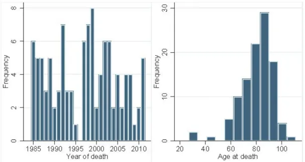
The distribution of the 106 sampled artist’s years of death (left panel) and their age at death (right panel) is shown in Figure 1. In the 24 years of our observation period 1985-2011, the number of cases of death varies between 0 and 8. The distribution of the age at death is more concentrated: the mean age at death is 80 and the median is 80.5.5
Figure 1: Distribution of death years and age at death for the 106 artists
4 We excluded 61 auction houses outside Europe and the US because they handled only very few sales of our sample artists’ work.
The left panel of Figure 2 shows that in our sample the number of auction sales increases after the artist’s death. This is the case for 75 of the 106 artists. The question therefore arises whether the artwork sold before and after the artists’ death differ.
Figure 2: Average number of artworks and mean auction price (corrected by the art index) around the year of death
Table 2 provides the descriptive statistics of the physical properties of the auctioned artwork, the auction houses handling the transactions, and the prices.
Table 1 Descriptive statistics of the 22,674 artworks of the 106 deceased artists
Mean Std. dev. Mean before Mean after Difference
Height (cm) 69.28 51.90 70.55 68.43 -2.12** Width (cm) 70.38 57.40 71.76 69.46 -2.30** Oil painting 0.45 0.47 0.44 -0.031*** Work on paper 0.42 0.43 0.42 -0.015** Print 0.13 0.10 0.14 0.048*** Signature 0.82 0.84 0.80 -0.03*** Christie’s 0.28 0.28 0.28 0.002 Sotheby’s 0.27 0.30 0.26 -0.04*** USA 0.48 0.50 0.47 -0.03*** Price (US $) 122,342 1,141,831 76,571 152,676 76,105***
In terms of dimension, the artwork is quite heterogeneous. The mean height and width amounting to about 70 cm are well in line with what most people are used to, but the standard deviation of more than 50 cm indicates a large variety of formats. 45% of the artwork in our sample are oil paintings, 42% are (unique) works on paper, the remaining 13% are prints. 82% of the artwork is
signed. The renowned auction houses Christie’s and Sotheby’s account for more than one half of all sales in our sample and almost one half of all auction sales were conducted in the United States, the other half in Europe. The differences in the reported means before and after the artists’ death are in eight of the nine reported characteristics statistically significant, but very small substantively. There is therefore no reason to suspect that the common trend assumption in differences-in-differences estimates is violated. The only before-and-after death difference that is statistically and substantively significant are the mean prices in US-dollars. They have doubled. The right panel of Figure 2 provides a more detailed picture of the price development around the year of death.
Measures of Artistic Reputation
We use the term artistic reputation in the sense of a quantitative measure of an artist’s acknowledged presence and notability in the art community. Measuring artistic reputation is not an easy task to begin with, but measuring artistic reputation at a specific point of time, in our case at the time immediately after the artist’s death, turns out to be a real challenge. Given these difficulties, we settled for employing a variety of measures based on different types of information, such as online sources, print media, and encyclopedias.
Online encyclopedias offer a readily available online source. We therefore collected from Wikipedia for each artist the number of languages in which they have entries. A second online-based measure of reputation we counted the number of books offered by amazon.com in the subcategories art history and biographies relating to the artists’ lives and artwork. Given that amazon is selling both new and used books, this measure includes books in stock as well as many out of print books.
The main problem with all online resources is that they do not lend themselves, at least not easily so, to measuring reputation at any given time in the past. Moreover, artists who died in the 1980s and 1990s may be less present in online fora and, since English is the predominant language of this medium, the online-based reputation measures of artists who have closer relations to the Anglo-Saxon world may be inflated. We therefore collected obituaries in general interest newspapers in different countries and base our preferred reputation measure on the number of
words in those obituaries.6 This measure is, in principle, well suited to measure the reputation of an artist at the time of death. We nevertheless acknowledge that this measure relies, for practical reasons, on a rather limited number of newspapers.
The standard measure of reputation used in the literature ranks the reputation of eminent persons by using word counts in entries of well-recognized, high-quality encyclopedias; Galenson (2006), for example, uses this method to rank artists, and Murray (2003) to rank extraordinary human accomplishments, in general. Those measures are highly objective because they reflect the so-called test of time; they do, however, not provide information about the reputation at the time of the persons’ death. In any event, we use for this purposes the Oxford Dictionary of Art and Artists (Chilvers 2017).7
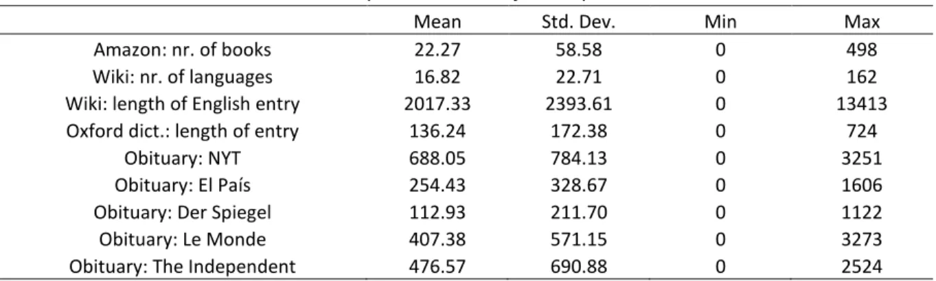
Table 3 reports some descriptive statistics for the nine reputation measures that we collected. The average number of amazon art books and biographies is 22 and the maximum number (Andy Warhol leads the pack) is almost 500 available books. For the average artist, Wikipedia provides information in about 17 different languages; in this contest Salvador Dalí wins with 162 different languages. Salvador Dalí also leads the field in the length of the English Wikipedia entry in all three languages that we considered. The longest obituaries commemorate Salvador Dalí, Marc Chagall, Willem de Kooning. The length of obituaries of the artists differ, mainly due to the preference for the “local” artists of the different newspapers.
Table 2: Descriptive statistics of our reputation measures
Mean Std. Dev. Min Max
Amazon: nr. of books 22.27 58.58 0 498
Wiki: nr. of languages 16.82 22.71 0 162
Wiki: length of English entry 2017.33 2393.61 0 13413
Oxford dict.: length of entry 136.24 172.38 0 724
Obituary: NYT 688.05 784.13 0 3251
Obituary: El País 254.43 328.67 0 1606
Obituary: Der Spiegel 112.93 211.70 0 1122
Obituary: Le Monde 407.38 571.15 0 3273
Obituary: The Independent 476.57 690.88 0 2524
6 The obituary measure is an arithmetic average of number of words in obituaries published in The New York Times, the German Der Spiegel, the Spanish El País, the French Le Monde, and the British The Independent.
7 We used the electronic version of this dictionary.
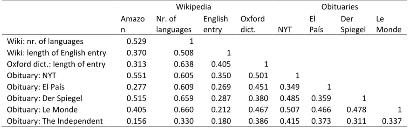
In most cases the correlation between our eight reputation measures is reasonably high (between 0.4 and 0.6, see Table 4). Exceptions are the measure based on the length obituaries in The Independent and the length of the English Wikipedia entry in some cases does not correlate well with the other measures. Nevertheless, the measure of inter-item similarity, Cronbach’s α, is quite high at 0.59. Similar correlations between different reputation measure have been found in Simonton (1984) for scientists. Simonton finds a reliability index of 0.78 based on 23 distinct measures of scientific reputation in a sample of over 2000 scientists spanning several centuries. This result should not be surprising given the study by Graddy (2013) who uses de famous Roger de Piles ranking to show that artists ranked by de Piles enjoy today a largely unchanged reputation – and that after three centuries.
Table 3: Correlations among the reputation measures
Wikipedia Obituaries
Amazon Nr. of languages English entry Oxford dict. NYT El País Der Spiegel Le Monde
Wiki: nr. of languages 0.529 1
Wiki: length of English entry 0.370 0.508 1
Oxford dict.: length of entry 0.313 0.638 0.405 1
Obituary: NYT 0.551 0.605 0.350 0.501 1
Obituary: El País 0.277 0.609 0.269 0.451 0.349 1
Obituary: Der Spiegel 0.515 0.659 0.287 0.380 0.485 0.359 1
Obituary: Le Monde 0.405 0.660 0.212 0.467 0.507 0.466 0.478 1
Obituary: The Independent 0.156 0.330 0.180 0.386 0.415 0.373 0.311 0.337
Note: Cronbach’s alpha is 0.59.
3.
Estimating the death effect
Empirical strategy
To estimate the causal effect of an artist’s death on the price of her artwork, we introduce the treatment variable
𝐷𝐷𝐸𝐸𝑖𝑖𝑖𝑖 = �
0 if age𝑖𝑖< death age𝑖𝑖 1 if age𝑖𝑖≥ death age𝑖𝑖
that indicates whether the creator 𝑚𝑚 of an artwork 𝑖𝑖 sold at auction was alive (𝐷𝐷𝐸𝐸𝑖𝑖𝑖𝑖 = 0) or dead
(𝐷𝐷𝐸𝐸𝑖𝑖𝑖𝑖 = 1) when the transaction took place. The treatment status, i.e. whether an artist is dead
or alive (𝐷𝐷𝐸𝐸), is thus a deterministic function of the artist’s age.
We consider two specifications for estimating the death effects. The first specification applies the regression discontinuity design (Angrist and Pischke 2014, ch. 4) and estimates the death effect for each artist individually:
ln𝑝𝑝̂𝑖𝑖 =𝛼𝛼0 +𝛾𝛾𝐷𝐷𝐸𝐸𝑖𝑖+𝑓𝑓(𝑎𝑎𝑖𝑖) +𝜀𝜀𝑖𝑖, where 𝑖𝑖= 1, … ,𝑛𝑛𝑖𝑖 (2)
In this specification, ln𝑝𝑝̂𝑖𝑖 is the log auction price (corrected for changes in an art price index and for hedonic characteristics of the sold artwork) of each of the pictures 𝑖𝑖 = 1, … ,𝑛𝑛𝑖𝑖created by artist 𝑚𝑚. In order to identify the parameter 𝛾𝛾, we control for the artist’s age with the help of function 𝑓𝑓(𝑎𝑎𝑖𝑖), where 𝑎𝑎 is the difference between the “running age” and the artist’s death age; 𝑎𝑎 is therefore negative as long as the artist is alive. We work with linear and quadratic functions
𝑓𝑓(𝑎𝑎𝑖𝑖) and also allow different 𝑓𝑓(𝑎𝑎𝑖𝑖)-coefficients on the both sides of the death threshold using an
interaction term 𝐷𝐷𝐸𝐸×𝑓𝑓(𝑎𝑎).
The second specification for estimating the death effect applies the difference-in-difference (DD) design (Angrist and Pischke 2014, ch. 5). In our DD approach we estimate the death effects using the entire panel of artists in our sample:
ln𝑝𝑝𝑖𝑖𝑖𝑖𝑖𝑖 = 𝛼𝛼0 + � 𝜇𝜇𝑖𝑖+ 68 𝑖𝑖=2 � 𝛾𝛾𝑖𝑖𝐷𝐷𝐸𝐸𝑖𝑖𝑖𝑖𝑖𝑖+� 𝛽𝛽𝑋𝑋𝑖𝑖𝑖𝑖𝑖𝑖𝑖𝑖 𝐾𝐾 𝑖𝑖=1 + 68 𝑖𝑖=2 � 𝛿𝛿𝑖𝑖𝑌𝑌𝑖𝑖+𝜀𝜀𝑖𝑖𝑖𝑖𝑖𝑖 2011 𝑖𝑖=1980 (3)
In this specification, the dependent variable ln𝑝𝑝𝑖𝑖𝑖𝑖𝑖𝑖 is the log hammer price of lot 𝑖𝑖 (sold in year
𝑡𝑡) of an artwork created by artist 𝑚𝑚. We regress these prices on 𝐾𝐾 hedonic characteristics included in matrix 𝑋𝑋. We also control for changes in general art market prices using the year dummies 𝑌𝑌𝑖𝑖 and include artist-specific linear time trends and artist fixed effects.
Estimation Results: Regression Discontinuity Design
In our regression discontinuity regressions, we use on the left hand side of equation (2) prices that are corrected for the hedonic characteristics of each item sold and for the general movements
of the art market. To arrive at these corrected or normalized prices, we estimated for each artist 𝑚𝑚 the following auxiliary regression:
ln𝑝𝑝�𝑖𝑖 = 𝛽𝛽0+𝜷𝜷𝑿𝑿𝑖𝑖 +𝜀𝜀𝑖𝑖 𝑤𝑤ℎ𝑒𝑒𝑒𝑒𝑒𝑒𝑖𝑖 = 1, … ,𝑛𝑛𝑖𝑖 (4)
where 𝑝𝑝�𝑖𝑖 is already the hammer price corrected for general price movements in the art market. To correct for these general price movements, we constructed a price index that is based on our entire price dataset of 20th century artists. Many studies of art price formation correct the art prices only for inflation. We do not favor this approach because it clearly ignores the specific price development of the art market. The dependent variable (ln𝑝𝑝�𝑖𝑖) in equation (4) is thus the auction hammer price divided by our own art price index.
The constant 𝛽𝛽0 is the artist-specific base price level and 𝜷𝜷 is a 𝑘𝑘× 1 vector of parameters measuring the influence of the hedonic characteristics on the hammer price of artwork 𝑖𝑖. The
𝑘𝑘×𝑛𝑛𝑖𝑖 matrix 𝑿𝑿 comprises the following variables: the log of the painting’s size (height width),
a signature dummy, medium dummies (oil, work on paper, print), dummies for the auction houses Sotheby’s and Christie’s (i.e. proxies for the quality of the artwork), and a dummy for European auction houses (the reference group being US based auction houses).
The corrected prices 𝑝𝑝̂𝑖𝑖 that we use in equation (2) are thus the residuals of the hedonic regressions (4). In Figure 3, we plot for our sample of 106 artists an average of the corrected prices against the normalized year of sale (defined as years before and after the respective artists’ death, i.e. the artist died in the normalized year of sale 0). The average that we use for this figure is the mean across all 106 artists of the mean corrected price for each individual artist. Figure 3 reveals an economically significant discontinuity in auction prices in the death year; the price increase amounts to more than 15%. This kind of averaging blurs, of course, individual heterogeneity in death effects. We depict therefore the individual corrected prices for twelve artists in Figure 4 (to be found at the end of the paper). The selection is meant to demonstrate the heterogeneity in death effects. A visual inspection of the twelve panels reveals that the corrected prices jump in the death year for some artists and remain constant for others.8 Economically
8The trend lines are not influenced by the observations in the death year (i.e. year zero), as for most of the artists
we do not have enough observations before and after death in the death year. The observations in the death year are, however, used in the regressions.
significant price increases appear to be associated with artists who died at a relatively young age. This is of course in line with our hypothesis derived from the Coase conjecture.
Figure 3: Average corrected auction prices across all artists against relative years of sale
One important lesson to be learned from Figures 3 and 4 is that the price trend over the normalized year of sale (i.e. our “running age” in equation 2) can be different on the two sides of the threshold. We thus consider in addition to specification (2) a specification that can accommodate different time trends before and after the artist’s death, i.e. a specification with an appropriate interaction term (Angrist and Pischke 2014):
ln𝑝𝑝̂𝑖𝑖 = 𝛼𝛼0 +𝛾𝛾𝐷𝐷𝐸𝐸𝑖𝑖+𝑓𝑓(𝑎𝑎𝑖𝑖) +𝛿𝛿[𝑓𝑓(𝑎𝑎𝑖𝑖)𝐷𝐷𝐸𝐸𝑖𝑖] +𝜀𝜀𝑖𝑖, where 𝑖𝑖 = 1, … ,𝑛𝑛𝑖𝑖 (5)
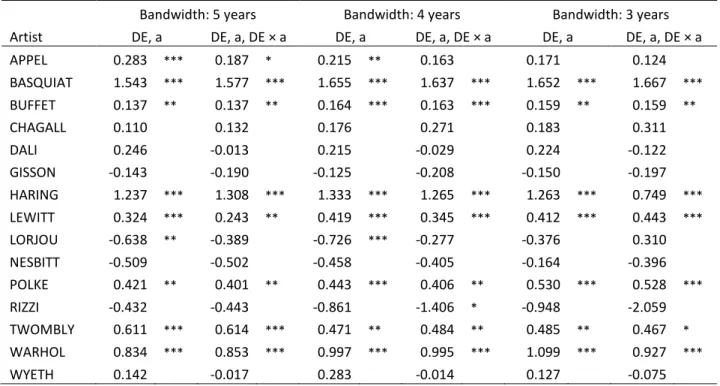
The results of the regression discontinuity regressions of specification (2) and (5) are reported for the twelve showcased artists in Table 5. We show results for three different bandwidths. The estimated death effects 𝛾𝛾, of specification (2), range from -0.64 to 1.54, indicating that the downward jump in auction prices can be about 64%, while the upward jump could reach more than 150%. However, for a large portion of the artists (31) we estimate statistically insignificant death effects in all specifications. Among the artist whose death has not induced a marked price
change we find also superstars such as Salvador Dali and Roy Lichtenstein. We discuss the potential determinants of these differences in death effects in Section 4.
Table 4: Regression discontinuity estimations of the death effect for 15 selected artists
Bandwidth: 5 years Bandwidth: 4 years Bandwidth: 3 years
Artist DE, a DE, a, DE × a DE, a DE, a, DE × a DE, a DE, a, DE × a
APPEL 0.283 *** 0.187 * 0.215 ** 0.163 0.171 0.124 BASQUIAT 1.543 *** 1.577 *** 1.655 *** 1.637 *** 1.652 *** 1.667 *** BUFFET 0.137 ** 0.137 ** 0.164 *** 0.163 *** 0.159 ** 0.159 ** CHAGALL 0.110 0.132 0.176 0.271 0.183 0.311 DALI 0.246 -0.013 0.215 -0.029 0.224 -0.122 GISSON -0.143 -0.190 -0.125 -0.208 -0.150 -0.197 HARING 1.237 *** 1.308 *** 1.333 *** 1.265 *** 1.263 *** 0.749 *** LEWITT 0.324 *** 0.243 ** 0.419 *** 0.345 *** 0.412 *** 0.443 *** LORJOU -0.638 ** -0.389 -0.726 *** -0.277 -0.376 0.310 NESBITT -0.509 -0.502 -0.458 -0.405 -0.164 -0.396 POLKE 0.421 ** 0.401 ** 0.443 *** 0.406 ** 0.530 *** 0.528 *** RIZZI -0.432 -0.443 -0.861 -1.406 * -0.948 -2.059 TWOMBLY 0.611 *** 0.614 *** 0.471 ** 0.484 ** 0.485 ** 0.467 * WARHOL 0.834 *** 0.853 *** 0.997 *** 0.995 *** 1.099 *** 0.927 *** WYETH 0.142 -0.017 0.283 -0.014 0.127 -0.075
The (DE, a) columns report estimates the DE from specification (2) and the (DE, a, DE × a) columns from
specification (5) that includes an interaction term of running age and death dummy. Full list of results is available on request. * p<0.10, ** p<0.05, *** p<0.01
Estimation Results: Difference-in-Difference Design
The second method that we employ to estimate individual death effects is the difference-in-difference (DD) estimator. Unlike RD, DD estimates the treatment effect not by directly exploiting the exogenous discontinuity caused by the artists’ death but by comparing the prices of the artwork of treated, i.e. deceased, artists with the prices of artwork created by artists who are still alive and thus can serve as a control group. This approach does not give rise to any objections if the assignment to the treatment and control groups is random because in this case the prices move in parallel, at least for sufficiently large treatment and control groups. Death is, of course, to a large extent a random event, but because expected mortality varies positively with age we need to establish that the pre-treatment price paths, i.e. the price paths of the artwork of living and deceased artists, do indeed move in parallel. Only if the pre-treatment time paths move
in parallel can we remove doubts about whether post-treatment differences in the two time paths indicate the treatment or death effect.
We estimate the death effect in the pseudo panel setting in which the control group consists of all auction sales of artwork created by the sample artists who are still alive. Since all of our sample artists die in the observation period and we only consider sales in the eleven-years of the time window around each artist’s death, the control group observations are taken from an ever changing and shrinking selection of living artist. In one of our robustness tests we therefore run the DD regression with other artists who were alive throughout the considered period.
The dependent variable in regression equation (3) is the raw log hammer prices of artist 𝑚𝑚’s artwork 𝑖𝑖 sold at auction in year 𝑡𝑡, ln𝑝𝑝𝑖𝑖𝑖𝑖𝑖𝑖. We use in this regression the raw prices because we control on the right hand side for art market idiosyncracies with time the fixed effects 𝑌𝑌𝑖𝑖, hedonic characteristics 𝑋𝑋𝑖𝑖𝑖𝑖𝑖𝑖𝑖𝑖 of the auctioned artwork, and with artist-specific fixed effects µ𝑖𝑖. The variables of interest are the artist-specific death dummies 𝐷𝐷𝐸𝐸𝑖𝑖𝑖𝑖𝑖𝑖. In line with Angrist and Pischke (2014), we refer to this setting as our multi-artist DD regression setup. Apart from using a different control group of artists, we can test the robustness of the estimated death effects by allowing for nonparallel trends in auction prices across artists. To do so, we amend equation (3) with artist specific linear time trends 𝜃𝜃𝑖𝑖𝑡𝑡:
ln𝑝𝑝𝑖𝑖𝑖𝑖𝑖𝑖 =𝛼𝛼0+ � 𝜇𝜇𝑖𝑖+ 106 𝑖𝑖=2 � 𝛾𝛾𝑖𝑖𝐷𝐷𝐸𝐸𝑖𝑖𝑖𝑖𝑖𝑖 +� 𝛽𝛽𝑋𝑋𝑖𝑖𝑖𝑖𝑖𝑖𝑖𝑖 𝐾𝐾 𝑖𝑖=1 + 106 𝑖𝑖=1 � 𝛿𝛿𝑖𝑖𝑌𝑌𝑖𝑖+ � 𝜃𝜃𝑖𝑖𝑡𝑡+ 106 𝑖𝑖=2 𝜀𝜀𝑖𝑖𝑖𝑖𝑖𝑖 2016 𝑖𝑖=1980 (6)
Using specification (6) also allows us to compare the DD with the RD estimates, as the RD specification (2) contains by construction a running variable.
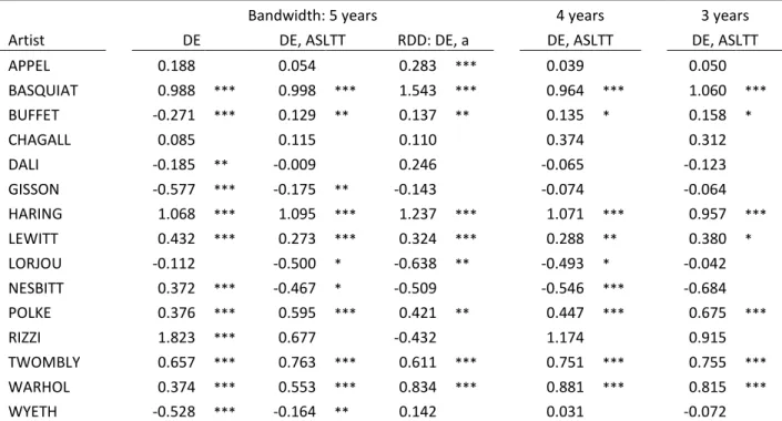
The results of our DD regressions are reported in Table 6. Comparing the first two columns, one can see that the estimates resulting from specifications (3) and (6) differ significantly for many artists. Moreover, many estimates in the first column imply sizable death effects which vanish when including artist-specific linear time trends (column 2). Our preferred specification is specification (6). In columns 4 and 6 we report the estimates of specification (6) for smaller bandwidths. Those estimates are largely in line with our preferred specification with a bandwidth
of 5 years (column 2). The estimates of our preferred specification (column 2) indicate statistically significant death effects 𝛾𝛾𝑖𝑖 ranging from -0.5 to 1.1, indicating price changes on impact between -50% and +110%. We conclude that the death effect is statistically significant for only about one half of our sample artists when considering specifications that include artist-specific linear time trends. This result is in line with our RD results. The death effects estimated with the RD method are also similar to those estimated with the DD method, however somewhat larger. The measure of similarity of all RD and DD estimates, Cronbach’s 𝛼𝛼, amounts to 0.94.
Table 5: Diff-in-diff estimations of the death effect for 15 selected artists
Bandwidth: 5 years 4 years 3 years
Artist DE DE, ASLTT RDD: DE, a DE, ASLTT DE, ASLTT
APPEL 0.188 0.054 0.283 *** 0.039 0.050 BASQUIAT 0.988 *** 0.998 *** 1.543 *** 0.964 *** 1.060 *** BUFFET -0.271 *** 0.129 ** 0.137 ** 0.135 * 0.158 * CHAGALL 0.085 0.115 0.110 0.374 0.312 DALI -0.185 ** -0.009 0.246 -0.065 -0.123 GISSON -0.577 *** -0.175 ** -0.143 -0.074 -0.064 HARING 1.068 *** 1.095 *** 1.237 *** 1.071 *** 0.957 *** LEWITT 0.432 *** 0.273 *** 0.324 *** 0.288 ** 0.380 * LORJOU -0.112 -0.500 * -0.638 ** -0.493 * -0.042 NESBITT 0.372 *** -0.467 * -0.509 -0.546 *** -0.684 POLKE 0.376 *** 0.595 *** 0.421 ** 0.447 *** 0.675 *** RIZZI 1.823 *** 0.677 -0.432 1.174 0.915 TWOMBLY 0.657 *** 0.763 *** 0.611 *** 0.751 *** 0.755 *** WARHOL 0.374 *** 0.553 *** 0.834 *** 0.881 *** 0.815 *** WYETH -0.528 *** -0.164 ** 0.142 0.031 -0.072
The DE column reports estimates of the DE from specification (3) and the DE, ASLTT columns from specification (6) that includes artist specific linear time trends (ASLTT). The RDD column duplicates the regression discontinuity results with bandwidth 5 years from Table 5. Full list of results is available on request. * p<0.10, ** p<0.05, *** p<0.01
Before testing in the next section whether the estimated artist-specific death effects follow the pattern predicted by microeconomic theory, we first turn to the interesting case of Keith Haring and acknowledge here that we did, so far, not reveal all pertinent facts when presenting the data and regression results relating to this famous artist who sadly died at a very young age.
Placebo estimates: The case of Keith Haring
Regression discontinuity and difference-in-differences designs go a long way towards establishing causal effects; in our case a causal effect of an artist’s death on the price change in her artwork. An even more exacting test of the underlying economic theory would be to show that when a case of death is “announced” for the near future, the market reacts in advance, i.e. at the time of the announcement and not after the fact. Given informed and rational market participants, this is what one would expect to happen because expected changes in fundamentals of asset pricing are priced in at once.
It does not happen very often that a case of death is “announced” for the near future. But in the case of Keith Haring this is exactly what happened. Haring rose to fame in the 1980s when he was in his twenties. He was diagnosed with AIDS in 1988, announced his affliction, and established his foundation to provide financial support for AIDS-related education, prevention, and care. He also used his art in the fight against AIDS. Since in the late 1980s no effective medical treatment against the immune deficiency was available, it was clear that Haring did not have long to live. With Haring’s announcement of his HIV-positive status, all actors in the art market knew that his life’s work would be smaller than hitherto expected. From a theoretical perspective, one would therefore expect that the announcement of his health status would have led to an immediate increase in the prices of his artwork. Given his reputation and his young age, Haring was not yet 32 years old when he died, one would furthermore expect this death effect to be extraordinarily large. This is exactly what happened: the prices of Haring’s pictures did not rise after his death in 1990, but already after the announcement of his incurable illness two years before. The death or in this case rather announcement effect illustrated in Figure 5 amounts to about 130% (see Table 5, column 2). Notice that in Haring’s case, the normalized year 0 in Figure 5 does not indicate his year of death (1990) but the year in which he made the announcement of his health status (1988).
To corroborate this finding, we employ the border-falsification strategy proposed by Becker et al. (2016) which, in turn, is derived from the regression discontinuity design (Imbens and Lemieux 2008). The basic idea of this strategy is not to consider time windows (or in the original context: geographical bands) that include the border line (in our case the border-line year) that is claimed to give rise to the discontinuity, because otherwise the placebo estimates would be flawed by the effects deriving from the border-line (in our case the announcement of Haring’s terminal illness).
Our time windows include 3 years before the announcement and 3 years after the announcement, i.e. we take our shortest time windows to test as close as possible to the true announcement year. In order not to cross the true announcement year, we test for the existence of the death effect in three consecutive years, namely 1993, 1994, and 1995. We could not test for the artificial death effect before the announcement year, because assuming a time window of three years, we would have to assume fictitious time windows that include the year 1985 and earlier years, i.e. years in which only very few pictures by Haring were sold at auctions (in 1985 Haring was, after all, only 27 years old).
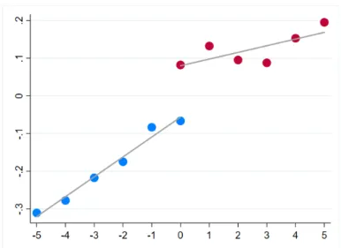
Figure 5 plots four death effects for Keith Haring. The first effect is the effect following the actual announcement in 1988, the three other effects assume, counterfactually, that the announcement had been made in 1993, 1994, and 1995. The true announcement effect indicates a statistically significant price increase of about 75% (see Table 5, column 6), the placebo death effects are very small and statistically not significant.
Figure 5: Estimates of Placebo Death Effects for Keith Haring
4.
Explaining the Death Effect: Reputation and Age at Death
The Coase conjecture and general asset pricing considerations give rise to two hypotheses that guided our attempts to explain the estimated heterogeneity in death effects across artists. The first
hypothesis maintains that that the death effect varies, ceteris paribus, negatively with the artist’s age at death and disappears for artists who die at a very high age. The ceteris paribus clause is important because the death of an aspiring young or middle-aged artist who is still little known by the general public, but who some insiders believe to be likely to make it big, may have a significant negative effect on the prices of her artwork because her death nips those hopes of becoming eminent in the bud and thus frustrates the expectations of the early collectors. For young and middle-aged artists who do not yet enjoy a generally acknowledged reputation in the art world, the positive death effect associated with the death-induced curtailment of their oeuvre is diminished by a negative effect associated with frustrated expectations of reputation. We thus hypothesize that the death effect of artists who die before their time is smaller, perhaps even negative, for less reputed artists than for truly eminent ones.
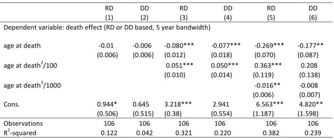
As an initial test of the first hypothesis we regress the estimated death effects of our sample artist on a polynomial of the respective artist’s age at death. We have two dependent variables: the death effects estimated with the regression discontinuity (RD) method and those estimated with the difference-in-difference (DD) method. In both cases we use the estimates obtained from the regressions based on the bandwidth of five years. Table 7 reports the results.
Table 6: The death effect as a function of age at death
RD DD RD DD RD DD
(1) (2) (3) (4) (5) (6)
Dependent variable: death effect (RD or DD based, 5 year bandwidth)
age at death -0.01 -0.006 -0.080*** -0.077*** -0.269*** -0.177** (0.006) (0.006) (0.012) (0.018) (0.070) (0.087) age at death2/100 0.051*** 0.050*** 0.363*** 0.208 (0.010) (0.014) (0.119) (0.138) age at death3/1000 -0.016** -0.008 (0.006) (0.007) Cons. 0.944* 0.645 3.218*** 2.941 6.563*** 4.820** (0.506) (0.515) (0.38) (0.554) (1.187) (1.598) Observations 106 106 106 106 106 106 R2-squared 0.122 0.042 0.321 0.220 0.382 0.239
All rows are based on the weighted least squares regression, with the underlying squared precisions as analytical weights. The RD columns use as dependent variable the death effects estimated from the Regression Discontinuity specification (2) with a 5-year bandwidth, i.e. Table 5, column 2. The DD columns use as dependent variable the death effects estimated from the Difference-in-Difference specification (6) with a 5-year bandwidth, i.e. Table 6, column 2. Robust standard errors in the parentheses.
The model fit is much better when using the death effects estimated with the RD method than when using the DD estimates. Given the significance of the all three powers of age at death in the regression reported in column (5), and also because the cubic functional form is less restricting that the quadratic specification, we proceed with this specification. The relationship between age at death and the death effect is illustrated in Figure 7 that plots the graphs of the preferred specification (cubic RD) and the cubic DD specification reported in Table 7. Both graphs have the shape predicted by our first hypothesis: the death effect is largest for artists who die at a young age and decreases with increasing age at death. The death effect remains positive for all artists who died before 60 and then disappears for artists who died after the age of 60.
Figure 7: Death effect as a cubic function of age at death Note: RD, Table 7, column 5; DD, Table 7, column 6
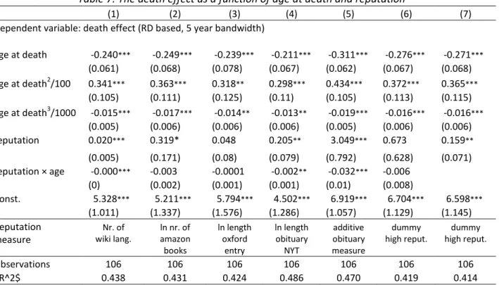
The storyline that relates the price jump following the death of young artists to the surprising and large curtailment of their oeuvre now needs to be enriched by the role of reputation. After all, the regression results reported in Table 7 lump together artists who enjoyed at the time of death different levels of reputation.9 To do so, we amend specification (5) in Table 7 with the measures of reputation discussed in Section 2. To capture the moderating effect of reputation predicted by our second hypothesis, we interact the variables REPUTATION and AGE-AT-DEATH. We report the results in Table 8. The effect of reputation is for all reputation measures positive,
9 The reason why we obtain in our estimates reported in Table 7 and plotted in Figure 7 a death effect that decreases with age at death whereas Ursprung and Wiermann (2011) and Etro and Stepanova (2015) obtained a hump-shaped curve can be attributed to the differences in the employed samples. Both Ursprung and Wiermann (2011) and Etro and Stepanova (2015) worked with very large samples which included a large number of artists with little or no reputation to speak of. Our sample, however, only includes artist whose work has been sold many times in a relatively short period which implies that all of our sample artists enjoy a substantial reputation.
however not significant for all measures. More importantly, because this lends empirical support to our second hypothesis, the estimated coefficient of the interaction term is negative, i.e. the effect of reputation decreases with age at death.
Table 7: The death effect as a function of age at death and reputation
(1) (2) (3) (4) (5) (6) (7)
Dependent variable: death effect (RD based, 5 year bandwidth)
age at death -0.240*** -0.249*** -0.239*** -0.211*** -0.311*** -0.276*** -0.271*** (0.061) (0.068) (0.078) (0.067) (0.062) (0.067) (0.068) age at death2/100 0.341*** 0.363*** 0.318** 0.298*** 0.434*** 0.372*** 0.365*** (0.105) (0.111) (0.125) (0.11) (0.105) (0.113) (0.115) age at death3/1000 -0.015*** -0.017*** -0.014** -0.013** -0.019*** -0.016*** -0.016*** (0.005) (0.006) (0.006) (0.006) (0.005) (0.006) (0.006) reputation 0.020*** 0.319* 0.048 0.205** 3.049*** 0.673 0.159** (0.005) (0.171) (0.08) (0.079) (0.792) (0.628) (0.071) reputation × age -0.000*** -0.003 -0.0001 -0.002** -0.032*** -0.006 (0) (0.002) (0.001) (0.001) (0.01) (0.008) Const. 5.328*** 5.211*** 5.794*** 4.502*** 6.919*** 6.704*** 6.598*** (1.011) (1.337) (1.576) (1.286) (1.057) (1.129) (1.145)
Reputation Nr. of ln nr. of ln length ln length additive dummy dummy
measure wiki lang. amazon
books oxford entry obituary NYT measure obituary high reput. high reput.
Observations 106 106 106 106 106 106 106
$R^2$ 0.438 0.431 0.424 0.486 0.470 0.419 0.414
All rows are based on the weighted least squares regression. The dependent variable is the death effects estimated from the Regression Discontinuity specification (2) with a 5-year bandwidth (see Table 5, column 2). The underlying squared precisions are used as analytical weights. The additive obituary measure is calculated as sum of relative obituaries lengths across all five magazines. The high reputation dummy is one if the obituaries were of exceptional lengths. * p<0.10, ** p<0.05, *** p<0.01
Using, for example, the reputation measure based on the number of books available on the amazon website (column 3), a 1% increase in the number of books dealing with the respective artist’s life or work, increases the death effect by 60%. If, however, such an eminent artist dies at the age of 85, this effect is reduced by about 62%. We illustrate the relationship between age at death and reputation in Figure 8, where we plot the graph of the function estimated in column (7) of Table 8. The reputation measure in this specification is a dummy variable derived from the number of words in our obituaries measure. We indicated 25 artists who had exceptionally long obituaries (longer than 450 words) as highly eminent at the time of their death, i.e. the dummy equals one for these 25 artists. For the remaining artists the high reputation dummy equals zero. In Figure 8, the age at death curve for highly eminent artist is above the curve for the less
eminent artists. Moreover, the death effect for the highly eminent artists becomes zero about 15 years later than for the less eminent artists.
Figure 8: Relationship between the death effect and age at death for highly reputed and reputed artists
5.
Conclusion
Empirical studies measuring and explaining death effects in the visual art market have hitherto used panel data to estimate average death effects, i.e. death effects that could not be associated with specific individual artists. In this study we estimate individual death effects for a sample of artists whose work has been sold at auctions sufficiently often to allow estimating artist-specific death effects with the help of regression discontinuity and difference-in-differences techniques. In our sample of 106 artists we find artists with statistically positive and negative death effects, as well as artists whose death caused no statistically significant death effect.
We explain this heterogeneity in death effects by applying the famous Coase (1972) conjecture to the art market. In the art market context, the Coase conjecture gives rise to two hypotheses that we test with our data. The first hypothesis maintains that death effects are negatively related to the deceased artists’ age at death and disappear when an artist dies at a high age. The second hypothesis predicts that for artists who die before their time, the death effects varies positively with the deceased artist’s reputation at the time of death.
Our results support all of these predictions. To test our hypotheses, we collected a variety of potential measures of artistic reputation. Our results turn out to be quite robust with respect to the
reputation measures used in explaining the variance in the observed individual death effects. The main conclusion that we draw from our results is that the basic predictions of asset pricing theory can be used to interpret art price formation; in other words, pieces of visual art exhibit fundamental characteristics of financial assets.
As compared to previous studies on the death effect, we disentangling for the first time the two of the main determinants of the death effect, to wit, age and artistic reputation at death. So far, empirical estimates of the relationship between the death effect and age and death has been confounded with influences arising from artistic reputation which, of course, to some extent correlated with age: young artists are less likely to be eminent than older ones. Since dying young, with little reputation but perhaps well-deserved hopes of eventually becoming an eminent artist, sets the stage for a negative death effects, the estimated relationship between the death effect and age at death turns out to be hump-shaped if one does not explicitly correct for reputation. When taking reputation into account, as we do in this study, the hump-shaped relationship between the death effect and age and death gives way to a negative relationship for young and middle-aged artists and vanishing death effects for older artist.
Notice, finally, that dying young increases, at impact, the market value of the deceased artist’s work only if the deceased young artist already enjoyed a great deal of reputation. If nobody has noticed her qualities, perhaps because there were none to be found, the price of her artwork does not change at all, and if some early collectors made a perhaps well-informed wager and bought some of her artwork at increasing prices, they will have a lot to regret. What this shows is that you cannot trust wordsmiths with economic matters. In short, Mark Twain in his story that prompted the preamble of this working paper, got it all wrong. Making money from an artist’s death is not easy. It may even involve murder, at least if you want to believe economist-turned-mystery-writer Marshall Jevons (2014).
References
Angrist, J. D. and J.-S. Pischke (2014). Mastering metrics: The path from cause to effect. Princeton University Press.
Ashenfelter, O. and K. Graddy (2006). Art auctions. Handbook of the Economics of Art and Culture 1, 909–945.
Becker, S. O., Boeckh, K., Hainz, C., & Woessmann, L. (2016). The empire is dead, long live the empire! Long‐run persistence of trust and corruption in the bureaucracy. The Economic Journal 126(590), 40-74.
Canudas-Romo, V. (2010). Three measures of longevity: Time trends and record values. Demography 47(2), 299–312.
Chilvers, I. (2017). The Oxford dictionary of art and artists (5 ed.). Oxford University Press. Coase, R. H. (1972). Durability and monopoly. The Journal of Law and Economics 15(1), 143–
149.
Ekelund, R. B., J. D. Jackson, and R. D. Tollison (2017). The economics of American art: Issues, artists and market institutions. Oxford University Press.
Etro, F. and E. Stepanova (2015). The market for paintings in Paris between rococo and roman- ticism. Kyklos 68(1), 28–50.
Galenson, D. W. (2006). Artistic capital. Routledge.
Galenson, D. W. and R. Jensen (2001). Young geniuses and old masters: The life cycles of great artists from Masaccio to Jasper Johns. Technical report, National Bureau of Economic Research.
Galenson, D. W. and B. A. Weinberg (2000). Age and the quality of work: The case of modern American painters. Journal of Political Economy 108(4), 761–777.
Galenson, D. W. and B. A. Weinberg (2001). Creating modern art: The changing careers of painters in France from impressionism to cubism. American Economic Review 91(4), 1063– 1071.
Graddy, K. (2013). Taste endures! the rankings of Roger de Piles († 1709) and three centuries of art prices. The Journal of Economic History 73(3), 766–791.
Imbens, G. and Lemieux, T. (2008). Regression discontinuity designs: a guide to practice, Journal of Econometric 142(2), 615–35.
Itaya, J. and H. W. Ursprung (2016). Price and death: modeling the death effect in art price formation. Research in Economics 70(3), 431–445.
Jevons, M. (2014). The mystery of the invisible hand. Princeton, Princeton University Press. Murray, C. (2003). Human accomplishment: The pursuit of excellence in the arts and sciences,
800 BC to 1950. Harper Collins.
Simonton, D. (1984). Scientific eminence historical and contemporary: A measurement assessment. Scientometrics 6(3), 169–182.
Ursprung, H. (2015). Zum Todeseffekt im Kunstmarkt (the death effect in the art market). In H. Bündge and J. Holten (eds.), Nach dem frühen Tod (after an early death), [bilingual], Staatliche Kunsthalle Baden-Baden, Walther König, Köln,104-113.
Ursprung, H. and C. Wiermann (2011). Reputation, price, and death: An empirical analysis of art price formation. Economic Inquiry 49(3), 697–715.
Table 8: Descriptive statistics of auctions by artist
Age at Nr. of auctions Average hammer price (US $)
Artist Death date death before after diff before after diff
APPEL, Karel 5/3/2006 85 347 662 315 37338 65067 27729
ARMAN, Fernandez 10/22/2005 77 134 318 184 12994 26259 13265
BACON, Francis 4/28/1992 82 11 30 19 2300000 640601 -1615245
BASQUIAT, Jean Michel 8/12/1988 27 67 241 174 13314 70586 57272
BERMUDEZ, Cundo 10/30/2008 94 34 33 -1 21301 53901 32600 BERNSTEIN, Theresa F 2/12/2002 111 22 50 28 3734 3946 212 BEUYS, Joseph 1/23/1986 64 11 46 35 5392 22710 17319 BOHROD, Aaron 4/3/1992 84 37 32 -5 2486 3000 514 BRATBY, John 7/20/1992 64 28 23 -5 1528 2297 768 BUFFET, Bernard 10/4/1999 71 386 352 -34 33978 26663 -7315 BURRI, Alberto 2/13/1995 79 21 44 23 76764 182489 105725 CADMUS, Paul 12/12/1999 94 56 52 -4 6685 15339 8655 CARRENO, Mario 12/20/1999 86 98 32 -66 55713 35329 -20384 CASCELLA, Michele 8/31/1989 96 57 62 5 3865 8210 4345 CESAR, Baldaccini 12/6/1998 77 33 53 20 2947 3035 87 CHAGALL, Marc 3/28/1985 97 144 346 202 91973 450482 358509 CHILLIDA, Eduardo 8/19/2002 78 31 124 93 14974 21115 6141 CLAVE, Antoni 9/1/2005 92 175 160 -15 28876 35852 6975 DALI, Salvador 1/23/1989 84 84 114 30 52566 75450 22883 DORAZIO, Piero 5/17/2005 77 234 408 174 9295 32964 23669 DUBUFFET, Jean 5/12/1985 83 166 423 257 29048 224160 195112 DYF, Marcel 9/15/1985 85 26 74 48 1704 5743 4039 DZUBAS, Friedel 12/10/1994 79 35 27 -8 12553 5143 -7410 EGGENHOFER, Nick 3/1/1985 87 53 13 -40 3747 7008 3261 EISENDIECK, Suzanne 6/15/1998 90 45 20 -25 2189 2355 166 ELLINGER, David 3/24/2003 90 44 60 16 1544 2689 1145
ERTE, Romain de Tirtoff 4/21/1990 98 68 66 -2 5167 4332 -835
FRANCIS, Sam 11/4/1994 71 240 293 53 102061 51142 -50919 FRANKENTHALER, Helen 12/27/2011 83 164 325 161 107644 132084 24440 FREUD, Lucian 7/20/2011 88 162 244 82 1000000 849150 -193375 FRINK, Elizabeth 4/18/1993 62 60 81 21 3229 3433 204 FROST, Terry 9/1/2003 87 107 293 186 5756 23564 17808 GALL, Francois 12/9/1987 75 70 144 74 2124 5285 3160 GISSON, Andre 7/28/2003 75 127 175 48 2216 2471 255 GRAVES, Morris 5/5/2001 90 35 28 -7 10934 22552 11618 GUAYASAMIN, Oswaldo 3/10/1999 79 38 31 -7 21746 26691 4944 GUTTUSO, Renato 1/18/1987 75 90 135 45 9559 18293 8734 HAMBOURG, Andre 12/4/1999 90 143 124 -19 6883 8097 1214 HAMILTON, Richard 9/13/2011 89 149 181 32 32885 28941 -3944 HARING, Keith 2/16/1990 32 56 200 144 4528 20248 15720 HARTUNG, Hans 12/8/1989 85 242 210 -32 38074 60436 22362
HAYTER, Stanley William 5/4/1988 86 27 40 13 3479 9048 5570
HELD, Al 7/27/2005 77 16 28 12 12350 39776 27426
HERON, Patrick 3/20/1999 79 18 52 34 5550 43807 38258
HIRSCHFELD, Al 1/20/2003 99 17 99 82 4356 6849 2493
IMMENDORF, Jorg 5/28/2007 61 97 129 32 19780 49179 29399
KINGMAN, Dong 5/12/2000 89 46 21 -25 2276 4093 1817 KIPPENBERGER, Martin 3/7/1997 43 5 67 62 3370 36737 33367 KITAJ, R. B. 10/21/2007 74 20 34 14 93738 65817 -27921 KLUGE, Constantine 1/9/2003 91 40 61 21 5201 4694 -508 KOONING, Willem de 3/19/1997 92 79 156 77 373222 350655 -22567 LE PHO 12/12/2001 94 78 94 16 7275 19980 12704 LEVIER, Charles 9/3/2003 83 64 52 -12 1231 1350 119 LEWITT, Sol 4/8/2007 79 205 399 194 13567 26281 12714 LICHTENSTEIN, Roy 9/29/1997 73 151 556 405 171558 95532 -76026 LORJOU, Bernard 1/26/1986 77 23 72 49 1547 5913 4365 LOVELL, Tom 6/29/1997 88 17 89 72 4500 13339 8839 LUCEBERT 5/10/1994 69 130 163 33 9200 6200 -3000 MANESSIER, Alfred 8/1/1993 81 79 53 -26 34798 9948 -24850 MARCA-RELLI, Conrad 8/29/2000 87 26 36 10 9378 19436 10057 MARTIN, Agnes 12/16/2004 92 48 37 -11 317036 1200000 833622 MASSON, Andre 10/28/1987 91 113 135 22 14737 58683 43947 MATTA, Roberto 11/23/2002 91 213 290 77 53287 73669 20382 MENKES, Zygmunt 8/20/1986 90 14 29 15 3679 3688 9 MITCHELL, Joan 10/30/1992 67 48 52 4 118490 102658 -15832 MOORE, Henry O M 8/31/1986 88 98 110 12 25750 34864 9114 MOTHERWELL, Robert 7/16/1991 76 99 80 -19 78949 42362 -36587 MUHL, Roger 4/4/2008 79 63 112 49 3983 4629 646 NESBITT, Lowell 7/8/1993 59 51 35 -16 2635 2123 -512 NOLAN, Sidney 11/28/1992 75 14 15 1 2603 47951 45348 NOLAND, Kenneth 1/5/2010 85 86 166 80 82795 156951 74156 OLITSKI, Jules 2/4/2007 85 23 84 61 33849 48596 14747
PAIK, Nam June 1/29/2006 73 12 34 22 10845 7362 -3483
PASMORE, Victor 1/23/1998 89 12 23 11 56256 19647 -36610 PIPER, John 6/28/1992 88 50 108 58 8945 6249 -2696 POLKE, Sigmar 6/10/2010 69 299 417 118 122813 474742 351929 PORTOCARRERO, Rene 4/27/1985 73 49 50 1 2460 5408 2948 RAUSCHENBERG, Robert 5/12/2008 83 174 143 -31 254506 556251 301745 RIOPELLE, Jean-Paul 3/12/2002 78 89 178 89 42304 136515 94211 RIVERS, Larry 8/14/2002 78 64 75 11 14473 40516 26042 RIZZI, James 12/26/2011 61 16 82 66 1571 1800 229 ROTH, Dieter 6/5/1998 68 37 90 53 3464 5001 1537
SAINT PHALLE, Niki de 5/21/2002 71 26 49 23 7421 7404 -17
SAURA, Antonio 7/22/1998 67 107 151 44 26266 34672 8406 SCANAVINO, Emilio 11/28/1986 64 11 81 70 1253 6659 5406 SCOTT, William 12/28/1989 76 31 22 -9 7142 15851 8709 SEBIRE, Gaston 12/13/2001 81 35 22 -13 2115 2327 212 SHEETS, Millard 3/31/1989 81 16 43 27 4294 6329 2035 SLOANE, Eric 3/5/1985 80 33 61 28 2294 4109 1815 SOYER, Raphael 11/4/1987 87 112 122 10 6103 6240 136 STAMOS, Theodoros 2/2/1997 74 74 62 -12 7439 7281 -158 STEINBERG, Saul 5/12/1999 84 67 49 -18 10736 12273 1537 TAMAYO, Rufino 6/24/1991 91 127 128 1 112195 226798 114603 TINGUELY, Jean 8/30/1991 66 42 86 44 10749 8637 -2112 TWOMBLY, Cy 7/5/2011 83 192 322 130 481648 1800000 1347472 VASARELY, Victor 3/15/1997 90 188 243 55 9707 9805 98
VENARD, Claude 1999 86 95 58 -37 1804 2675 871 VOSTELL, Wolf 4/3/1998 65 13 26 13 3394 3008 -386 WARHOL, Andy 2/22/1987 58 98 535 437 26686 117579 90893 WESSELMANN, Tom 12/17/2004 73 408 342 -66 33222 282873 249650 WIEGHORST, Olaf 4/27/1988 88 24 44 20 7341 13656 6315 WOLVECAMP, Theo 10/11/1992 67 17 67 50 6970 4653 -2317 WYETH, Andrew 1/16/2009 92 69 133 64 401728 222784 -178943 ZORNES, Milford 2/24/2008 100 92 50 -42 3317 2018 -1299 ZUNIGA, Francisco 8/9/1998 86 113 55 -58 6365 6700 335