Variable Selection in Mixture Models with an Uncertainty Component

Micha Schneider, Wolfgang Pößnecker, Gerhard Tutz

Variable Selection in Mixture Models with

an Uncertainty Component

Technical Report Number 225, 2019 Department of Statistics

University of Munich

Variable Selection in Mixture Models with an

Uncertainty Component

Micha Schneider, Wolfgang P¨oßnecker, Gerhard Tutz

Ludwig-Maximilians-Universit¨at M¨unchen Akademiestraße 1, 80799 M¨unchen

August 6, 2019

Abstract

Mixture Models as CUB and CUP models provide the opportunity to mo-del discrete human choices as a combination of a preference and an uncer-tainty structure. In CUB models the preference is represented by shifted binomial random variables and the uncertainty by a discrete uniform distri-bution. CUP models extend this concept by using ordinal response models as the cumulative model for the preference structure. To reduce model complexity we propose variable selection via group lasso regularization. The approach is developed for CUB and CUP models and compared to a stepwise selection. Both simulated data and survey data are used to inves-tigate the performance of the selection procedures. It is demonstrated that variable selection by regularization yields stable parameter estimates and easy-to-interpret results in both model components and provides a data-driven method for model selection in mixture models with an uncertainty component.

Keywords: Mixture Models; Variable Selection; lasso, CUB model; CUP model

1 Introduction

Mixture models are widely used to model heterogeneity in populations. D’Elia and Piccolo (2005) proposed a mixture type model for ordinal responses that accounts for the psychological process of human choices. The model has been investigated and extended in a series of papers for example by Piccolo and D’Elia (2008), Iannario and Piccolo (2012b) and Iannario and Piccolo (2012a). The ba-sic concept of the so-called CUB model is that the choice of a response category is determined by a mixture of feeling and uncertainty. Feeling refers to the de-liberate choice of a response category determined by the preferences of a person

while uncertainty refers to the inherent individual’s indecision. The first com-ponent is modelled by a binomial distribution, the latter by a discrete uniform distribution across response categories. An introduction and overview is given in Piccolo and Simone (2019). The CUP model described in Tutz et al. (2017) and further developed by Tutz and Schneider (2019) extends this concept by using any ordinal model as the cumulative model for the preference structure.

In this type of models the right choice of covariates is essential to get sensible models. Even for a moderate number of covariates simple methods as all-subset selection are too time consuming so that other techniques are in demand. Using penalization techniques as lasso by Tibshirani (1996) can overcome this issue. Previous work on variable selection in mixtures focused on mixtures of normal densities and mixtures where the weights do not depend on covariates. Khalili and Chen (2007) used the lasso approach for mixture models and chose a penalty function which is proportional to the mixture weight. Further work was done by Luo et al. (2008) who propose to penalize the coefficients within and between Gaussian components and St¨adler et al. (2010) focus on high dimensional settings wherep >> n. But regularization has not been used to investigate the structure of CUB and CUP models with a specific discrete component and weights that depend on individual-specific covariates. In the following we show how to adopt the lasso framework to CUB and CUP models and compare the approach to a forward selection procedure.

The article is organized as follows. First, in section 2 the models are briefly described. In section 3 we discuss variable selection by a step procedure and the proposed lasso method, followed by section 4 about computational aspects of estimation, initialization and convergence. In section 5 we provide results of a simulation study and in section 6 we use the SHIW and ALLBUS survey to show the applicability of the methods on two real data problems. Finally the results are summarized.

2 Model Class

Let the probability that an individual i chooses the category r from ordered categories {1, . . . , k} given explanatory variableszi,xi be composed of the

indi-vidual’s propensity towards uncertainty and preference structure. The mixture distribution has the general form

P(Ri =r|xi) =πiPM(Yi =r|xi) + (1−πi)PU(Ui =r), (1)

where πi is the propensity or mixture weight, PM(Yi = r|xi) is a model for

the preference, and the uncertainty component PU(Ui = r) is determined by

a uniform distribution with probability 1/k for each response category. The uncertainty is assumed to include all kinds of indecision related to the nature of human choices like willingness to respond, lack of time, partial understanding

etc. The probability πi is assumed to be linked to covariates by the logit model

logit (πi) = zTi β, i= 1,2, . . . , n . (2)

The CUB and CUP models, used in this article, only vary in the choice of the preference component. The preference structure in CUB models (combination of uncertainty and binomial) is modelled by a shifted binomial distributionbr(.)

with parameterξ, that is,

br(ξi) = k−1 r₋1 ξ_ik−r(1−ξi)r−1, r ∈ {1, . . . , k},

whereξi is linked to the covariates xTi by

logit (ξi) = γ0+xiTγ, i= 1,2, . . . , n . (3)

The so called CUP model (combination of uncertainty and preference), descri-bed in Tutz et al. (2017), uses any ordinal model. A traditional model is the cumulative logit model

log P(Yi ≤r|xi) P(Yi > r|xi) =γ0r+xTi γ, r = 1, . . . , k−1.

(see Agresti, 2013; Tutz, 2012). The CUP models are more flexible and can handle complex ordinal data structures. However, the intercept parameters depend on the number of categories k so that more parameters have to be estimated. Both models use covariates to model the preference structure and the weights. In general the covariateszi andxi may be identical, completely different or overlap.

It should be mentioned that the omission of the uncertainty component typically yields biased parameter estimates.

3 Variable Selection

Since there are two sets of covariates, variable selection is an major issue in mixture models. Let _X contain all possible variables which can be selected for the two independent sets ofz and x, which are linked to the parametersβ and

γ, respectively. It is typically not known which variables are relevant for the weights (z) and which for the preference structure (x) so that variable selection has to handle two separate effect structures. We propose a variable selection based on penalty terms that are tailored to the problem of selecting variables in two components and compare it with a stepwise procedure.

3.1 Stepwise Variable Selection

Two traditional methods are the forward and backward selection. The latter allows that all available explanatory variables are included in both components and the model complexity is reduced stepwise. Especially in mixture models too many possibly correlated covariates can lead to model degeneracy and conver-gence problems so that the estimates in the fit are hardly trustworthy or the complete model can not be fitted.

Alternatively, one might use a forward search procedure. Here the selection pro-cess starts with a basic model as the intercept model. In the first step all models with one covariate in any part of the model are fitted. Then the model with the strongest improvement in terms of a specific criterion is selected. In the next step the procedure continues with this selected model and all remaining covari-ates are evaluated. The procedure continues until no improvement is detected. In each step a covariate is assigned to only one of the two variable setsz and x. If a covariate is selected for one of the two sets, it is still possible that the same covariate is selected for the other variable set later. Several criteria can be used:

AIC(βˆ,γˆ) = −2l(βˆ,γˆ) + 2df(βˆ,γˆ), BIC(βˆ,γˆ) = ₋2l(βˆ,γˆ) +log(n)df(βˆ,γˆ),

or the likelihood-ratio test with

lq =−2[l0(βˆ,γˆ)−l(βˆ,γˆ)]

a

∼χ2(|df(βˆ,ˆγ)−df0(βˆ,γˆ)|),

where the likelihood of the previous model is compared to the likelihood of the enlarged model. Since the likelihood-ratio test uses the difference of deviances we refer to it also as “deviance” criterion. That variable is selected that yields the largest improvement in AIC or BIC or the smallest p-value of the likelihood-ratio test. If there are several p-values that are numerically close to zero, the model with the largest deviance difference is selected. When the AIC/BIC does not improve or the p-value of the likelihood-ratio test is larger than 0.05 the forward selection is terminated. The estimation of these models is performed as described in Section 4.1. The initializations and convergence checks are described in detail in section 4.2.

Backward/forward strategies have the disadvantage that they are rather variable. The instability of stepwise regression models was demonstrated, for example, by Breiman (1996). Moreover, the standard errors computed for the final model are not trustworthy because they simply ignore the model search. The larger the available number of variables the more models have to be estimated so that these techniques may not work well for very large data sets.

3.2 Variable Selection by Penalization

We propose to use a version of the lasso (Tibshirani, 1996) that is adapted to the mixture models to obtain a procedure that is not limited by the number of variables and produces stable results. The penalized log-likelihood that is to be maximized is given by

lp(β,γ) =l(β,γ)−J_λ(β,γ),

where l(β,γ) denotes the un-penalized log-likelihood and J_λ(β,γ) is a specific penalty term that enforces the selection of variables in both model components. Let the vectors zi and xi be partitioned into zTi = (zTi1, . . . ,zTig) and xTi =

(xT

i1, . . . ,xTih) such that each components refer to a single variable. For example,

the vector zij can represent all the dummy variables that are linked to the j-th

variable, or represent the power functions of thej-th variable if one includes poly-nomial terms. The corresponding predictors arezT

i βandxTi γwith corresponding

partitioning of the parameter vectors,βT = (βT₁, . . . ,βT_g) andγT _{= (γ}T

1, . . . ,γTh),

respectively. Then the proposed penalty has the form

J_λ(β,γ) = λβ g X j=1 q df_β jkβjk2+λγ h X j=1 q dfγjkγjk2, (4) whereλβ and λγ are the tuning parameters for the selection ofxand zvariables,

respectively. The weightsdf_β

j are defined as the number of parameters collected in the corresponding parameter vectorβ_j, the weightsdf_γjare defined in the same way. kk2 is the unsquared L2-Norm so that the penalty enforces the selection of

variables in the spirit of the group lasso (Yuan and Lin, 2006) rather than selection of single parameters.

All covariables have to be standardized to ensure that the selection of variables does not depend on their scale. Categorical variables have to be orthonormalized. The parameters λβ, λγ can be used to enforce specific selection properties. If

λβ → ∞ no explanatory variables are included in the mixture component and

selection is restricted to the effect of explanatory variables on the structured response. If λγ → ∞ no explanatory variables are included in the structured

response part and selection is confined to the mixture component. If no specific structure is pre-specified λβ, λγ can take any value and can be chosen in a data

driven way. A simplification that is tempting is to set λβ = λγ. It might be

sufficient in some applications but it should be used with care.

To select a certain model the use of a selection criterion is needed. In mixture models cross validation can be very time consuming so that we propose the use of AIC or BIC,

AIC(βˆ,γˆ) =₋2l(βˆ,γˆ) + 2edf(βˆ,γˆ), BIC(βˆ,γˆ) =₋2l(βˆ,γˆ) +log(n)edf(βˆ,γˆ),

whereedf(βˆ,ˆγ) is the effective degrees of freedoms of the mixture model. For each parameter setβˆandγˆ the effective degrees of freedoms are calculated separately by

edf(βˆ,γˆ) =edf(βˆ) +edf(γˆ) = 1 + g X j=1 edf(βˆj) +I+ h X j=1 edf(γˆj),

where 1 refers to the interceptβ0 andI to the number of interceptsγ0. The

CUB-model consist of 1 + 1-intercepts and the CUP-CUB-model of 1 + (k ₋1)-intercepts.

g and h denote the number of the penalized variables. Following Yuan and Lin (2006) the effective degrees of freedom of each variable are computed by

edf(βˆj) =1(kβˆjk2 >0) + (df_β j −1) kβˆjk2 kβˆM L j k2 , edf(ˆγj) =1(kγˆjk2 >0) + (dfγ_j −1) k ˆ γjk2 kγˆM L j k2 .

If a variable is not penalized theedf are identical to df_β

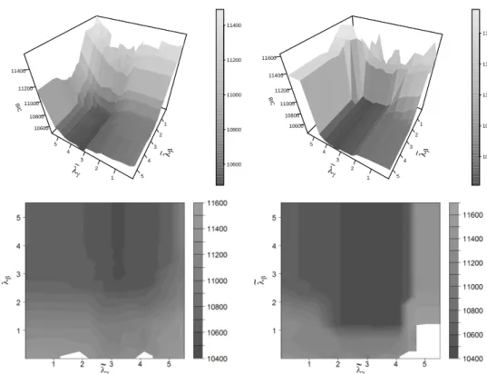
j and dfγj, respectively. To find the best model the procedure has to be optimized with reference to all sensible combinations of the tuning parametersλβ and λγ. We focus on the BIC

criterion to find the best model with the lowest BIC value. A two-dimensional grid of λ-values is investigated and parallelized in the following way. One di-mension is kept fixed while the other didi-mension is varied. By repeating this line search all combinations of tuning parameters are covered. For example, using a 15_×15 grid results in a 15 times 1_×15 line. The advantage of this approach is that we can use parallized computing architecture but also include the results of the previous model for the initialisation of the current model. This saves com-puting time and leads to non-degenerated results because the fit of the current model should be close to the fit of the previous model with a slightly different tuning parameter. Nevertheless we still use several random initialisations which are described in Section 4.2 to ensure that the fit is not conditioned on the pre-vious results.

Using a complete random choice of tuning parameter combinations can be pa-rallelized even better, but previous knowledge about model results can not be included easily. Another promising approach is the use of model based optimiza-tion as described in Bischl et al. (2017) to replace the more time consuming grid search.

4 Computational Aspects

4.1 Estimation with the EM-Algorithm

The mixture models considered in the previous sections can be estimated by an adapted version of the EM algorithm proposed by Dempster et al. (1977). Given the observed category yi the likelihood contribution of observation i is

P r(yi|zi,xi) = πiPM(yi|xi) + (1−πi)PU(yi) yi ∈ {1, . . . , k} (5)

yielding the log-likelihood

li(β,γ) = {log(πi) + log(PM(yi|xi))}+{log(1−πi) + log(1/k)}

The corresponding penalized log-likelihood is obtained by including the proposed penalty term yielding

li(β,γ) = {log(πi) + log(PM(yi|xi))}+{log(1−πi) + log(1/k)}

−λβ g X j=1 q df_β jkβjk2−λγ h X j=1 q dfγjkγjk2, and for all observations

lc(β,γ) = n X

i=1

[{log(πi) + log(PM(yi|xi))}+{log(1−πi) + log(1/k)}]

−λβ g X j=1 q df_β jkβjk2−λγ h X j=1 q dfγjkγjk2.

The EM algorithm uses the complete likelihood treating the membership to the uncertainty or structure component as missing data. Let z∗_i take the value 1 if observationibelongs to the structure component and zero if observationibelongs to the uncertainty component. Then the complete penalized log-likelihood is given by

lp(β,γ) = n X

I=1

z_i∗{log(πi) + log(PM(yi|xi))}+ (1−zi∗){log(1−πi) + log(1/k)}

−λβ g X j=1 q df_β jkβjk2−λγ h X j=1 q df_γjkγ_jk2,

where the probabilityπi depends on the individual characteristics by

πi = 1/(1 +e−z

T iβ).

Within the EM algorithm the log-likelihood is iteratively maximized by using an expectation and a maximization step. During the E-step the conditional

expectation of the complete log-likelihood given the observed data y and the current estimate θ(s) _{= (β}(s)_,γ(s)_),

M(θ_|θ(s)) = E(lp(θ)|y,θ(s))

has to be computed. Because lp(θ) is linear in the unobservable data z∗i, it

is only necessary to estimate the current conditional expectation of z∗

i. From

Bayes’s theorem follows

E(z∗i|y,θ) = P(zi∗ = 1|yi,xi,θ)

=P(yi|zi∗ = 1,xi,θ)P(zi∗ = 1|xi,θ)/P(yi|xi,θ)

=πiPM(yi|xi,θ)/(πiPM(yi|xi) + (1−πi)1/k) = ˆzi∗.

This is the posterior probability that the observationyi belongs to the structure

component of the mixture. For the s-th iteration one obtains

M(θ_|θ(s)) = n X i=1 n ˆ z∗(s) i log(πi) + (1−zˆ∗ (s) i ) log(1−πi) o −λβ g X j=1 q df_β jkβjk2 | {z } M1 + n X i=1 n ˆ z∗(s) i log(PM(yi|xi) + (1−zˆ∗ (s) i ) log(1/k) o −λγ h X j=1 q dfγjkγjk2 | {z } M2

M1 andM2 can be estimated independently from each other but most traditional

methods, such as Fisher-Scoring, can not be used because the derivatives do not exist. This problem can be solved with the fast iterative shrinkage-thresholding algorithm (FISTA) of Beck and Teboulle (2009) which is implemented in the MRSP package by P¨oßnecker (2019) and is used for the maximisation problem of β and γ, which can be formulated generally as

ˆ θ= argmax θ∈Rd lp(β,γ) = −argmin θ∈Rd lp(β,γ) = argmin θ∈Rd − l(β,γ) +J_λ(β,γ). (6) FISTA belongs to the class of proximal gradient methods in which only the unpe-nalized log-likelihood and its gradient is necessary. The solution for the unknown parametersθ of the unpenalized log-likelihood in iteration t+ 1 is given by:

ˆ

θ(t+1) = ˆθ(t)+ 1

ν∇l( ˆθ

(t)_),

where ν > 0 is the inverse stepsize parameter. This estimator converges to the ML estimator so that each update of ˆθ(t) _{can be considered as an one-step}

used to define a searchpoint u. To motivate the procedure with penalty the equation (6) is reformulated by Lagrange duality to

ˆ

θ = argmin

θ∈C

(₋l(θ)),

where C = {θ ∈ Rd_|J

λ(β,γ) ≤ λ} is the constraint region corresponding to

J_λ(β,γ). Given u, the proximal operator associated with the penalty J_λ(θ) is then defined by P(u) = argmin θ∈Rd 1 2kθ−uk 2_+J λ(θ) and leads to ˆ θ(t+1) =_Pλ ν( ˆθ (t)₊ 1 ν∇l( ˆθ (t)_).

In a first step the penalty is ignored and a step toward the ML estimator via first-order methods creates a search point. Then this search point is projected onto the constraint region C to account for the penalty term. A detailed description is given in Tutz et al. (2015).

For given θ(s) _{one computes in the E-step the weights ˆz∗}(s)

i and in the M-step

maximizesM(θ|θ(s)_{) (or ratherM}

1 and M2), which yields the new estimates

β(s+1) = argmaxβ n X i=1 n ˆ z∗(s) i log(πi) + (1−zˆ∗ (s) i ) log(1−πi) o −λβ g X j=1 q df_β jkβjk2 γ(s+1) = argmax_γ n X i=1 ˆ z∗(s) i log(PM(yi|xi))−λγ h X j=1 q df_γjkγ_jk2.

The E- and M-steps are repeated alternatingly until the difference lp(θ(s+1))−

lp(θ(s)) is small enough to assume convergence. To account for different sizes of

the log-likelihood we define

lp(θ (s+1)_)−l p(θ(s)) rel.tol/10 +_|lp(θ(s+1))| < rel.tol

as stopping criteria. rel.tol is the relative tolerance which has to below a certain value, such as 1e−6, to assume convergence. λβ and λγ span a two-dimensional

grid of tuning parameter space. Dempster et al. (1977) showed that under weak conditions the EM algorithm finds (only) a local maximum of the likelihood function. Hence it is sensible to use meaningful start values to find a good solution of the maximization problem, which is described in the next section 4.2.

4.2 Initialization and Convergence

Using meaningful starting values is a crucial point in mixture models. Misspeci-fied starting values can lead to degenerated results, can be time consuming and can lead to poor estimation results. In the literature several methods were propo-sed as described in Baudry and Celeux (2015) and Karlis and Xekalaki (2003). In the random setting several random start values are chosen and all models are run until convergence. Then the best fit is selected. In the small EM strategy a large number of short runs are evaluated which do not have to converge completely. Only the model with the best fit is run until full convergence.

We use a special version of the small EM that refers to the model class con-sidered here so that we use several different configurations. The mixture model components are restricted to two components so that for every observation only

πi and its complement 1−πi need to be chosen which has to sum up to 1. From

experience we know that the mean weight for the uncertainty component (1₋π¯) is in most cases between 0.1 and 0.4. By using this information we are able to create meaningful scenarios which are more likely to be close to a realistic so-lution. The first strategy is to use a fixed weight for all πi, i = 1, . . . , n. Here

we chose πi = 0.9 and πi = 0.7 which correspond with a realistic weight for the

uncertainty component (1₋πi) of 0.1 and 0.3, respectively.

The second strategy is drawing the weightsπi so that they are not constant for

all observations. For example if we choose the value 0.7 and its complement 0.3 we assign randomly one of this two values toπi. Because of the randomness we repeat

the sample strategy at least two times for the chosen value resulting in two weight vectorsπ1,π2. To ensure that we have obtained different realizations we calculate

for each observation the quadratic difference between π1 and π2 and compute

the sum over all observations. If π1 and π2 are identical the computed sum is

zero so thatπ2 would be replaced by a new random sample. As a rule of thumb

the overall sum has to be larger than 0.1_·n to acceptπ2 as a valid initialization.

Thus, the sample strategy produce several weight vectors for one chosen value. Here we used 0.9 as well as 0.7 leading to four different initializations. Together with the two constant initializations we obtain at least six configurations which are run until small convergence defined as rel.tol < 0.01 or until the maximal numbers of em-iterations equal to 60 depending on which criteria is reached first. The one with the best result is selected and is run until complete convergence (rel.tol<1e₋6 or maximal numbers of em-iterations equal to 200). One E- and one M-step is defined as one em-iteration.

Every time the model is called we use at least these six configurations re-gardless if we use the stepwise selection or the penalization. In the latter we may also include another weight initialization. As described in section 3.2 we use a line search to find the best tuning parameter combination. Thus from the second position onwards we can use the computed weights of the previous tuning parameter combination as initialization for the current weights. Since at the

be-ginning of each line search less information about a realistic model is available, we use more configurations for initialization. It consists of the constant choice and two samples of the values 0.6,0.7,0.8 and 0.9.

Dempster et al. (1977) showed that the EM-algorithm converges to a local maximum which is measured in this models by a small difference in the (penali-zed) Likelihood. A priori we have little information about the exact geometrical shape of the likelihood so that in practice several problems may be occur.

It is well known that the speed of convergence is slow near to the maximum. If the density close to the maximum is very flat we experienced that the difference criterion in the (penalized) likelihood may be too strong. So the rule of likelihood difference is supplemented by a maximum number of em-iterations which can be used. Since the number of em-iterations is in most cases a backstop rule, we usually use a higher number of possible em-iterations which we think should usually not be reached. An exception is the initialization part of the algorithm where the algorithm should not run until complete convergence.

In some cases the (penalized) likelihood may jump between several values without approaching a maximum. This can be solved by adjusting the step-size or, if necessary, taking the best values even if the criterion of small differences in likelihood is not completely reached.

If the starting values are too close to the maximum it may happen that the algorithm diverges from the maximum or a good solution. For this case we implemented some checks to ensure that the best composition is used instead of using a solution which is worse but satisfying the criterion of small difference in (penalized) likelihood. During the EM-algorithm we keep the last ten results to be able to jump back to a previous solution. If this problem occurs between different starting values we select the next best solution. On the other hand we also want to allow the algorithm to search for a better solution. So we allow the algorithm to carry on after a dis-improvement of the likelihood in the first six em-iterations. If the algorithm still does not detect a better likelihood we jump back to the best solution found so far.

On rare occasions the parameters found may be close to the edge of the parameter space. Especially if almost all estimated mixture weights are close to zero or one. In this case we imposed a threshold of 1e₋06 to prevent the weights of being exact zero or exact one. Nevertheless if all mixture weights are close to one for one of the two components a mixture model may be questionable. In case of doubt we recommend to have a look at the estimated mixture weights.

The difference in the (penalized) likelihood is the main criteria of convergence. Only in the case of non-regular behaviour other criteria may be used. Different starting values not only help to find the best maximum but also help to avoid degenerated results.

5 Simulation

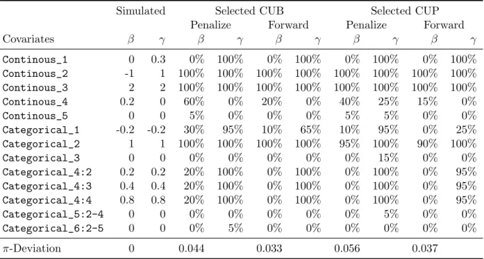
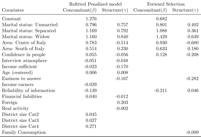
To illustrate whether the two selection methods are able to select the “true” covariates we use simulated data with effects and white noise variables with no effects. Forn= 3000 observations and k = 5 response categories we generate five metric covariates from a standard normal distribution (N(0,1)) and six categori-cal covariates. We use the same 11 covariates for xand z, but the effects differ. The first two columns of Table 1 contain the exact values forβ andγ used in the simulation. We want to use almost all possible combinations so that some effects of β and γ are identical and some differ. Also the covariates with no effect are sometimes identical (e.g. Continous_5) and in other cases there is an effect for only one of the parameters β and γ (e.g. Continous_1+4). In both parameter sets there are two continuous and three categorical covariates with no effects.

We use also relative small parameter values to create a realistic setting and to examine whether the size of the effect may have an impact on the different selection methods. The effects of the continuous covariates are 0.2, 0.3, 1, −1 and 2. Three categorical covariates are binary with the effect strength ₋0.2, 1 and 0. The other three categorical covariates consist of four, four and five categories. Only for the first of them we use effect sizes different from zero namely 0.2, 0.4 and 0.8. The other multi-categorical variables are white noise. The constants in the CUP model are ₋2.391,₋1.221,₋0.259,1.023 and in the CUB model₋1.5.

We generate S = 20 samples from the CUP- and CUB-model each following the described structure and selected variables with the penalization approach and forward selection. For the CUB and CUP model we present in Table 1 the number of times the covariate was selected depending on the used selection technique and the model. The last row includes theπ-deviations, which measure the difference between the estimated individual mixture weightsπ and the true values, defined by π-Deviation = 1 S S X j=1 1 n n X i=1 |πij −πˆij| ! ,

where S is the number of simulated data sets, n the number of observations in each data set, πij is the true mixture weight of the i-th observation in the j-th

simulation, and ˆπij is the corresponding estimated mixture weight. We compute

the absolute differences on each individual mixture weight and use the average over all observations and all samples as a measurement of discrepancy.

Both the penalization and forward selection technique show good results. Both techniques selected covariates with clear effects (−1,1 and 2) in almost 100% and show worse performance with smaller effect size of the parameters. But the penalization technique selected more often covariates with smaller effect size than the forward selection. For example looking at Categorical_1 the penalization technique selected these covariates in 30% and 95% of the cases in the CUB mo-del compared with only 10% or 65% of the cases using forward selection. The

Table 1: Result of simulated data

Simulated Selected CUB Selected CUP

Penalize Forward Penalize Forward

Covariates β γ β γ β γ β γ β γ Continous_1 0 0.3 0% 100% 0% 100% 0% 100% 0% 100% Continous_2 -1 1 100% 100% 100% 100% 100% 100% 100% 100% Continous_3 2 2 100% 100% 100% 100% 100% 100% 100% 100% Continous_4 0.2 0 60% 0% 20% 0% 40% 25% 15% 0% Continous_5 0 0 5% 0% 0% 0% 5% 5% 0% 0% Categorical_1 -0.2 -0.2 30% 95% 10% 65% 10% 95% 0% 25% Categorical_2 1 1 100% 100% 100% 100% 95% 100% 90% 100% Categorical_3 0 0 0% 0% 0% 0% 0% 15% 0% 0% Categorical_4:2 0.2 0.2 20% 100% 0% 100% 0% 100% 0% 95% Categorical_4:3 0.4 0.4 20% 100% 0% 100% 0% 100% 0% 95% Categorical_4:4 0.8 0.8 20% 100% 0% 100% 0% 100% 0% 95% Categorical_5:2-4 0 0 0% 0% 0% 0% 0% 5% 0% 0% Categorical_6:2-5 0 0 0% 5% 0% 0% 0% 0% 0% 0% π-Deviation 0 0.044 0.033 0.056 0.037

same behaviour applies for the CUP model. The selection of the β-parameters, which are linked to the mixture weights, seem to be more difficult for both se-lection techniques than the sese-lection of theγ-parameters. TheContinous_1and

Continous_4are characterized by nearly the same effect size (0.3 and 0.2), but differ very much in their selection frequency. While Continous_1 was selected for γ in 100% correctly, the covariate Continous_4 was only selected in 60% at the most correctly for theβ-parameter. Similar consequences can be drawn from the covariateCategorical_4. The covariate was selected in almost 100% of the cases for γ, but very rarely forβ.

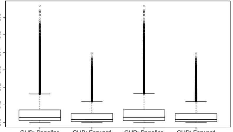
Table 2 summarizes the results of Table 1 by investigating how often effects that are zero and effects that are different from zero are detected correctly by the two selection methods. The forward selection technique never selected covariates with a true effect of zero while the penalization approach shows small false positive rates. However, the penalization approach performs distinctly better in detecting variables that have a non-zero effect. Both methods show lower rates in detecting effects for β than for γ.

The computed π-deviations displayed in Table 1 are very small for both se-lection methods given the average size of the simulatedπ = 0.8011 and that both selection methods are not always able to select all covariates correctly. Figure 1 displays the original deviations for all samples resulting in 60,000 observations in each boxplot. Most of them are very close to zero. The penalty approach shows