Solutions of Seventh Order Boundary Value Problems Using Ninth Degree Spline Functions and Comparison with Eighth Degree Spline Solutions

http://dx.doi.org/10.4236/jamp.2016.42032

Solutions of Seventh Order Boundary

Value Problems Using Ninth Degree Spline

Functions and Comparison with Eighth

Degree Spline Solutions

Parcha Kalyani, Mihretu Nigatu Lemma

School of Mathematical & Statistical Sciences, Hawassa University, Hawassa, Ethiopia

Received 10 June 2015; accepted 19 February 2016; published 22 February 2016

Copyright © 2016 by authors and Scientific Research Publishing Inc.

This work is licensed under the Creative Commons Attribution International License (CC BY).

http://creativecommons.org/licenses/by/4.0/

Abstract

In this article, we develop numerical method by constructing ninth degree spline function using extended cubic spline Bickley’s method to find the approximate solution of seventh order linear boundary value problems at different step lengths. The approximate solution is compared with the solution obtained by eighth degree splines and exact solution. It has been observed that the approximate solution is an excellent agreement with exact solution. Low absolute error indicates that our numerical method is effective for solving high order linear boundary value problems.

Keywords

Seventh Order Boundary Value Problem, Boundary Value Problem, Ninth Degree Spline Function, Absolute Error

1. Introduction

Consider the linear seventh order differential equation

( )7

_{( )}

_{( ) ( ) ( )}

y x + f x y x =r x

with the boundary conditions

( )

0 ,

( )

n ,

( )

0 ,

( )

n ,

( )

0 ,

( )

n ,

( )

0 .

y′′ x =α′′ y′′ x =β′′ y′′′ x =α′′′

Generally, this problem is difficult to solve analytically. Several numerical and semi-analytical methods have been developed for solving high order boundary value problems. For instance, a different approach of solving linear two-point boundary value problem has first been suggested by Bickley in 1968 [1]. He used cubic spline interpolation to model the solution curve and applied the differential equation as well as the boundary conditions to solve for the unknown constants. As a result, a set of equations can be produced approximating the analytical solution. Numerical methods based on spline functions generate solutions of ordinary and partial differential equations of high accuracy. The first place that the word “spline” is used in connection with smooth, piecewise polynomial approximation with mathematical reference has been made in the year 1946 by Schoenberg [2]. In late 1960’s, there were no handful of articles mentioning spline functions. Maclaren [3], Rubin and Khosla [4], Sastry [5], Schoenberg [6] made great contributions in the development of splines. Convergence properties of the cubic spline method have been discussed by Ahlberg and Nilson [7]. Univariate splines have been studied intensely in 60’s. By the mid 70’s, splines were well understood to permit a fairly comprehensive treatment in the form of books. Some of the books which discuss splines include Ahlberg et al. [8], deBoor [9], Prenter [10], Schumaker [11], Shikin and Plis [12], Spath [13]. The earlier studies [14]-[16] employed spline functions for the smooth approximate solution of ordinary and partial differential equations. Spline functions of various degrees have been demonstrated by them using approximate methods of solving second, third, fourth and fifth order li-near boundary value problems. There are number of research articles published on this subject, yet it remains an active research area. Techniques such as quadratic, cubic, quartic, quintic, sextic, septic and higher degree splines are used to discuss the numerical solution of linear and nonlinear BVPs. Kumar and Srivastava [17] have given a survey on recent spline techniques for solving boundary value problems in ordinary differential equa-tions using cubic, quintic and sextic polynomial and non-polynomial splines. Thomas [18] presents extensive use of splines for Boeing.

In the present paper, the seventh order boundary value problems are solved using ninth degree spline ap-proximation and compared with the solution obtained by eighth degree spline solution [19].

2. Construction of Ninth Degree Spline

We divide the interval

[

x x0, n

]

into n subintervals with grid points x x x x0, 1, 2, 3,,xn, starting at x0, the func-tion y(x) in the interval

[

x x0, 1

]

is represented by ninth degree spline S(x), which is an approximate solution of

y(x).

( )

(

) (

)

(

)

(

)

(

)

(

)

(

)

(

)

(

)

2 3 4 5

0 0 0 0 0

6 7 8 9

0 0 0 0 0

– – – – –

– – – –

S x a b x x c x x d x x e x x g x x h x x j x x k x x l x x

= + + + + +

+ + + +

proceeding to the next interval

[

x x1, 2

]

, we add a term

(

)

9 1 – 1

l x x , proceeding in to the next interval

[

x x2, 3

]

we add another term l2

(

x–x2

)

9 and so on until we reach xn. Thus the function y(x) is represented in the form

( )

(

) (

)

(

)

(

)

(

)

(

)

(

)

(

)

(

)

2 3 4 5

0 0 0 0 0

1

6 7 8 9

0 0 0

0

– – – – –

– – – –

n

i i

i

S x a b x x c x x d x x e x x g x x h x x j x x k x x l x x

−

=

= + + + + +

+ + + +

_∑

(1)

It can be shown that S(x) and its first six derivatives are continuous across nodes.

Method of Obtaining the Solution of Seventh Order Boundary Value Problems Using Ninth Degree Spline Function

Consider the linear seventh order differential equation

( )7

_{( )}

_{( ) ( )}

y x + f x y x =rx (2)

( )

( )

( )

( )

( )

( )

( )

0 0 0 0 , , , , , , . n n n

y x y x y x y x y x y x y x

α β α β

α β α

′ ′ ′ ′

= = = =

′′ = ′′ ′′ = ′′ ′′′ = ′′′ (3)

From (3), and taking spline approximation in (2) at x=xi for i=0,1, 2, 3, 4,,n, we get (n + 8) equations in (n + 9) unknowns a b c d e g h j k, , , , , , , , , l l l0, , ,1 2,ln−1. To have the solution for the unknowns one more

eq-uation is required. So we assume that ln−1=ln−2, after determining these unknowns we substitute them in (1) and

thus we get ninth degree spline approximation of y x

( )

. Putting x=x x x1, 2, 3,,xn in the spline function thus determined we get the solution at the grid points. The system of equations to be satisfied by the coefficients

, , , , , , , , ,

a b c d e g h j k l l l₀, , ,_{1 2},l_n−1 is derived below. From Equation (1) we get

( )

7

5040 40320

s x = j+

( )

(

)

1

(

)

2

7

0 0

5040 40320 181440 ni i i

s x = j+ x−x +

∑

₌−l x−x (4)

Substituting (1) and (4) in the differential Equation (2) at x=xm we get

(

)

(

)

(

)

(

)

(

)

(

)

(

)

(

)

(

)

(

)

(

)

2 3 4 5

0 0 0 0 0

6 7 8

0 0 0 0

9 1

0 0

0

5040 40320

181440 , 0,1, 2, ,

m m m m m m m m m m m m

m m m m m m m m

n

i m m m m

i

S af bf x x cf x x df x x ef x x gf x x

hf x x j f x x k f x x x x r

l f x x x x r m n

− = = + − + − + − + − + −     + − + _ − + _+ _ − + − _   +

∑

_ − + − _ = _ (5)

where fm= f x

( )

m ,rm=r x

( )

m and sm =S x

( )

m .

Since S(x) approximates y x

( )

, from (1) and from the boundary conditions (3) we obtain

,

a=α (6)

(

) (

)

(

)

(

)

(

)

(

)

(

)

(

)

(

)

2 3 4 5

0 0 0 0 0

1

6 7 8 9

0 0 0

0 – – – – – – – – – n i i i

a b x x c x x d x x e x x g x x h x x j x x k x x l x x β

−

=

+ + + + +

+ + + +

∑

= (7)

,

b=α′ (8)

(

)

(

)

(

)

(

)

(

)

(

)

(

)

(

)

2 3 4 5

0 0 0 0 0

1

6 7 8

0 0

0

2 3 4 5 6

7 8 9

n

i i

i

b c x x d x x e x x g x x h x x j x x k x x l x x β

−

=

+ − + − + − + − + −

′

+ − + − +

∑

− = (9)

2c=α′′ (10)

(

)

(

)

(

)

(

)

(

)

(

)

(

)

2 3 4

0 0 0 0

1

5 6 7

0 0

0

2 6 12 20 30

42 56 72

n

i i

i

c d x x e x x g x x h x x j x x k x x l x x β

− = + + − + − + − + − ′′

+ − + −

∑

− = (11)

6d=α′′′ (12) From (5)-(12) we have (n + 8) equations, if these equations are taken in the order (7), (9), and (11) with

, 1, , 0

m=n n−  , (12), (10), (8) and (6) the coefficient matrix of the unknowns, l ln,?n−1 l l1 0, k, j, h, g, e, d, c,

b, a will be an upper triangular matrix with two lower sub diagonals. The forward elimination is then simple with only two multipliers at each step, and back substitution is correspondingly easy.

3. Numerical Illustrations

3.1. Example 1

Consider the linear non homogeneous seventh order boundary value problem with constant coefficients.

( )

( )

(

)

7 2

ex 35 12 2 , 0 1

u x = −u x − x+ x+ x ≤ ≤x (13)

With the boundary conditions

( )

( )

( )

( )

( )

( )

( )

2 3

2

0 0, 0 1, 0 0, 0 3

1 0, 1 e, 1 4e

u u u u

u u u

′

= = = = −

′

= = − = − (14)

The exact solution is

( ) (

1

)

e .x u x =x −x

We find the solution of (13)-(14) by taking step lengths h = 0.2 and h = 0.1 at equal subintervals.

Solution with h = 0.2

The ninth degree spline S(x) which approximates y(x) is given by

( )

(

) (

)

(

)

(

)

(

)

(

)

(

)

(

)

(

)

2 3 4 5

0 0 0 0 0

6 7 8 4 9

0 0 0 i0i i

S x a b x x c x x d x x e x x g x x h x x j x x k x x ₌l x x

= + − + − + − + − + −

+ − + − + − +

∑

− (15)

where x0=0, x1=0.2, x2 =0.4, x3=0.6, x4=0.8, x5=1.

We have 13 unknowns a b c d e g h j k l l l l l, , , , , , , , , , , , ,0 1 2 3 4 and the conditions to be satisfied by these unknowns

are

( )

( )

( )

( )

( )2

_{( )}

( )2

_{( )}

( )3

_{( )}

0 5 0 5

0 0, 5 0, 1, e, 0, 4e, 0 3

S x = S x = S x′ = S x′ = − S x = S x = − S x = −

( )

( )

(

)

7 2

exi 35 12 2 , for 0,1, 2, 3, 4.

i i i i i

s x = −S x − x + x + x i= (16)

Since S x

( )

0 =0, S x′

( )

0 =1, S′′

( )

x0 =0,

( )3

_{( )}

0 3

S x = − , it follows that a = 0, b = 1, c = 0 and d = −0.5, hence the spline S(x) reduces to the form

( ) (

)

(

)

(

)

(

)

(

)

(

)

(

)

(

)

3 4 5 6

0 0 0 0 0

7 8 4 9

0 0 0

0.5

i i

i

S x x x x x e x x g x x h x x j x x k x x ₌l x x

= − − − + − + − + −

+ − + − +

∑

− (17)

Differentiating (17)

( )

(

)

(

)

(

)

(

)

(

)

(

)

(

)

2 3 4 5

0 0 0 0

6 7 4 8

0 0 0

1 1.5 4 5 6

7 8 9 _{i i}

i

S x x x e x x g x x h x x j x x x x ₌l x x

′ = − − + − + − + −

+ − + − +

∑

− (18)

( )

(

)

(

)

(

)

(

)

(

)

(

)

(

)

2 3 4

0 0 0 0

5 6 4 7

0 0 0

3 12 20 30

42 56 72 _{i i}

i

S x x x e x x g x x h x x j x x k x x ₌l x x

′′ = − − + − + − + −

+ − + − +

∑

− (19)

( )

(

)

(

)

(

)

(

)

(

)

(

)

2 3

0 0 0

4 5 4

0

6

0 0

3 24 60 120

210 336 504 _i

i i

S x e x x g x x h x x j x x k x x ₌l x x

′′′ = − + − + − + −

+ − + − +

∑

− (20)

and the seventh derivative is

( )

(

)

(

)

2

7

0

4 0

5040 40320 181440

i i i

s x = j+ k x−x +

∑

₌l x−x (21) Solving set of equations obtained from (16) we get the following values,

0.333336938451

e= − , k= −0.001189612320, l3= −0.000104846937

0.124993192353

0.033335683705

h= − , l1= −0.000069129326

0.006944444444

j= − , l2= −0.000059468625

Substituting these values in Equation (15) we get the spline approximation S x

( )

of u x

( )

.

[image:5.595.99.503.115.568.2] [image:5.595.138.486.312.571.2]

The values of S x

( )

, u x

( )

and the corresponding absolute errors at x x x x1, 2, 3, 4 have been given in the

Table 1 and the comparison has been shown inFigure 1.

Solution with h = 0.1

Since h = 0.1 we suppose the grid points x0, x1, x2, x3, x4, x5, x6, x7, x8, x9, x10, where, x0 = 0, x1 = 0.1, x2 = 0.2, x3 = 0.3, x4 = 0.4, x5 = 0.5, x6 = 0.6, x7 = 0.7, x8 = 0.8, x9 = 0.9, x10 = 1.

From Equation (1) ninth degree spline S(x) which approximate s u(x) becomes

( )

(

) (

)

(

)

(

)

(

)

(

)

(

)

(

)

(

)

2 3 4 5

0 0 0 0 0

6 7 8

0

9

0 0 0

9

i i i

S x a b x x c x x d x x e x x g x x h x x j x x k x x ₌l x x

= + − + − + − + − + −

+ − + − + − +

∑

− (22)

From Equation (22) and the boundary conditions we get the following values

0.333329053989

e= − , l0= −0.002337817833, l5 =0.004265136252

0.125006230461

g= − , l1=0.004280966493, l6= −0.004351989532

0.033377848548

h= − , l2= −0.004334132039, l7=0.003471663012

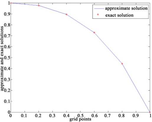
[image:5.595.89.537.609.721.2]

Figure 1. Comparison of approximate solution and exact solution for example 1 with h = 0.2.

Table 1. Numerical solution S x

( )

, exact solution u x

( )

and absolute error of example 1with h = 0.2.

x S(x) u(x) Absolute Error

0.0 0.00000000000 0.000000000000 0.000000000

0.2 0.19542437561 0.195424441305 3.74400E−09

0.4 0.35803789382 0.358037927433 3.36110E−08

0.6 0.437308436394 0.437308512093 7.56990E−08

0.8 0.356086488213 0.356086548558 6.03450E−08

0.006944444444

j= − , l3=0.004274000045, l8 = −0.001235877131

0.000219994881

k= − , l4= −0.004341991663, l9= −0.001235877131

Substituting these values in Equation (22) we get the spline approximation S x

( )

of u x

( )

. The values of

( )

[image:6.595.135.496.225.484.2]

S x , u x

( )

and the corresponding absolute errors at x1, x2, x3, x4, x5, x6, x7, x8, x9, x10 have been given in the

Table 2and the comparison has been shown inFigure 2.

3.2. Example 2

Consider non-homogeneous linear seventh order boundary value problem with variable coefficients

( )

( )

(

)

7 2

ex 2 6 , 0 1

[image:6.595.87.538.514.721.2]

u x =xu x + x − x− ≤ ≤x (23)

Figure 2. Comparison of S x

( )

and u x

( )

for example1 with h = 0.1.

Table 2. Numerical solution S x

( )

, exact solution u x

( )

and absolute error of example 1 with h = 0.1.

x S(x) u(x) Absolute Error

0.0 0.000000000000 0.000000000000 0.00000000

0.1 0.099465382958 0.099465382626 −3.3200E−10

0.2 0.195424444859 0.195424441305 −3.5540E−09

0.3 0.283470361956 0.283470349590 −1.2366E−08

0.4 0.358037954657 0.358037927400 −2.7224E−08

0.5 0.412180361425 0.412180317675 −4.3750E−08

0.6 0.437308566741 0.437308512093 −5.4648E−08

0.7 0.428881204050 0.42888068568 −5.1837E−08

0.8 0.356086581653 0.356086548558 −3.3095E−08

0.9 0.221364288517 0.221364280004 −8.5130E−09

Subject to the boundary conditions

( )

( )

( )

( )

( )

( )

( )

0 1, 0 0, 0 1, 0 3

1 0, 1 e, 1 2e

u u u u

u u u

′ ′′ ′′′

= = = − = −

′ ′′

= = − = − (24)

The exact solution is

( ) (

1

)

e .x u x = −x

We find the solution of (23)-(24) by taking the step lengths h = 0.2 and h = 0.1 at equal sub intervals.

Solution when h = 0.2

Since h = 0.2 we suppose the grid points x0 =0, x1=0.2, x2=0.4, x3=0.6, x4 =0.8, x5 =1

From Equation (1) ninth degree spline S(x) which approximates u(x).

( )

(

) (

)

(

)

(

)

(

)

(

)

(

)

(

)

(

)

2 3 4 5

0 0 0 0 0

6 7 8

0

9

0 0 0

4

i i i

S x a b x x c x x d x x e x x g x x h x x j x x k x x ₌l x x

= + − + − + − + − + −

+ − + − + − +

∑

− (25)

From S(x) and boundary conditions we get the following values.

a = 1, b = 0, c = −0.5, d = −0.333333 Equation (25) reduces to the form

( )

(

)

(

)

(

)

(

)

(

)

(

)

(

)

(

)

2 3 4 5

0 0 0

4 0

0

6 7 8 9

0 0 0

1 0.5 0.333333

i i i

S x x x x x e x x g x x h x x j x x k x x ₌l x x

= − − − − + − + −

+ − + − + − +

∑

− (26)

From equation

( )

( )

0

(

)

7

0 0 0

2 0

0 e 2 6

x

s x −x u x = x − x −

we get j = −0.00119047619047 and from the remaining conditions we have the following values 0.125011015552

e= − , j= −0.001190476190, l1= −0.000004737182, l4= −0.000004658016

0.033311297448

g= − , k= −0.000173008441, l2= −0.000003893449

0.006956208579

h= − , l0= −0.000024317513, l3= −0.000004658016

[image:7.595.185.443.496.703.2]

Substituting these values in Equation (25) we get the spline approximation S(x) of u(x). The values of S(x), u(x) and the corresponding absolute errors at x1, x2, x3 and x4 has been given inTable 3 and the comparison has been shown in Figure 3.

[image:8.595.88.541.99.221.2]

Table 3. Numerical solution S(x), exact solution u(x) and absolute error of example 2 with h = 0.2.

x S(x) u(x) Absolute Error

0.0 1.000000000000 1.000000000000 0.00000000

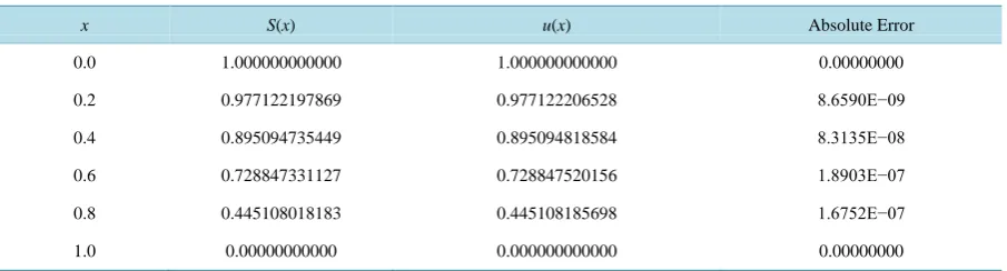
0.2 0.977122197869 0.977122206528 8.6590E−09

0.4 0.895094735449 0.895094818584 8.3135E−08

0.6 0.728847331127 0.728847520156 1.8903E−07

0.8 0.445108018183 0.445108185698 1.6752E−07

1.0 0.00000000000 0.000000000000 0.00000000

Solution when h =0.1

Since h = 0.1 we suppose the grid points x0, x1, x2, x3, x4, x5, x6, x7, x8, x9, x10 where

x0 = 0, x1 = 0.1, x2 = 0.2, x3 = 0.3, x4 = 0.4, x5=0.5, x6 = 0.6, x7 = 0.7, x8 = 0.8, x9 = 0.9, x10 = 1 From Equation (1) ninth degree spline S(x) which approximates u(x) becomes

( )

(

) (

)

(

)

(

)

(

)

(

)

(

)

(

)

(

)

2 3 4 5

0 0 0 0 0

6 7 8

0

9

0 0 0

9

i i i

S x a b x x c x x d x x e x x g x x h x x j x x k x x ₌l x x

= + − + − + − + − + −

+ − + − + − +

∑

− (27)

From S(x) and boundary conditions we get the following values.

a = 1, b = 0, c= −0.5, d = −0.333333, with these values (27) reduces to the form

( )

(

)

(

)

(

)

(

)

(

)

(

)

(

)

(

)

2 3 4 5

0 0 0

9 0

0

6 7 8 9

0 0 0

1 0.5 0.333333

i i i

S x x x x x e x x g x x h x x j x x k x x ₌l x x

= − − − − + − + −

+ − + − + − +

∑

− (28)

proceeding as in the above, we get the following values

0.125049990637813

e= − , l0= −0.000025112018076, l5= −0.000000909345915

0.033253352807342

g= − , l1=0.000000834757197, l6= −0.000007629408480

0.006977804974566

h= − , l2= −0.000006702827825, l7= −0.000003171741363

0.001190476190

j= − , l3=0.000000146740426, l8= −0.000008022104888

0.000172613927990

k= − , l4= −0.000007470638178, l9= −0.000008022104888

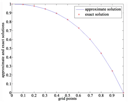
The values of S(x), u(x) and the corresponding absolute errors at x1, x2, 𝑥𝑥3, x4, x5, x6, x7, x8, x9, x10 has been given in Table 4 and the comparison has been shown inFigure 4.

3.3. Example 3

Consider the linear non-homogeneous seventh order boundary value problem with constant coefficients.

( ) ( )

7

7e , 0x 1

u x =u x − ≤ ≤x

subject to the boundary conditions

( )

0 1,

( )

0 0,

( )

0 2,

( )

1 0,

( )

1 e,

( )

1 2e

u = u′ = u′′ = − u = u′ = − u′′ = − (29)

The exact solution is

( ) (

1

)

e .x u x = −x

We find the solution of (29) by taking the step lengths h = 0.2 and h = 0.1 at equal sub intervals.

[image:9.595.185.450.82.286.2] [image:9.595.188.440.310.486.2]

Figure 4. Comparison of approximate solution and exact solution of example 2 with h = 0.1.

Figure 5. Comparison of approximate solution and exact solution of example 3 with h = 0.2.

[image:9.595.185.444.511.704.2]

[image:10.595.85.539.101.289.2]

Table 4. Numerical solution S(x), exact solution u(x) and absolute error of example 2 with h = 0.2.

x S(x) u(x) Absolute Error

0.0 1.000000000000 1.000000000000 0.000000000

0.1 0.994653825368 0.994653826268 9.00000E−10

0.2 0.977122206669 0.977122206528 2.98590E−10

0.3 0.944901160432 0.944901165303 4.87100E−09

0.4 0.895094814647 0.895094818584 3.93700E−09

0.5 0.824360636278 0.824360635350 −9.28000E−10

0.6 0.728847525865 0.728847520156 −5.70900E−09

0.7 0.604125874632 0.604125812241 −6.23910E−08

0.8 0.445108198680 0.445108185698 −1.29820E−08

0.9 0.245960300626 0.245960311115 1.04890E−08

[image:10.595.88.533.316.429.2]

1.0 0.000000000000 0.000000000000 0.000000000

Table 5. Numerical solution S(x), exact solution u(x), absolute error of example 3 with h = 0.2.

x S(x) u(x) Absolute Error

0.0 1.000000000000 1.000000000000 0.000000000

0.2 0.977122202945 0.977122206528 3.58300E−09

0.4 0.895094784979 0.895094818584 3.36050E−08

0.6 0.728847097431 0.728847520156 4.22725E−07

0.8 0.44510798551 0.445108185698 1.71470E−07

[image:10.595.87.538.450.643.2]

1.0 0.00000000000 0.000000000000 0.000000000

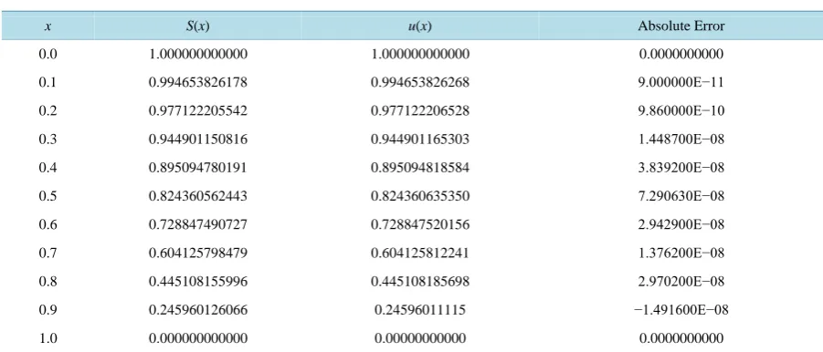
Table 6. Numerical solution S(x), exact solution u(x) and absolute error of example 3 with h = 0.1.

x S(x) u(x) Absolute Error

0.0 1.000000000000 1.000000000000 0.0000000000

0.1 0.994653826178 0.994653826268 9.000000E−11

0.2 0.977122205542 0.977122206528 9.860000E−10

0.3 0.944901150816 0.944901165303 1.448700E−08

0.4 0.895094780191 0.895094818584 3.839200E−08

0.5 0.824360562443 0.824360635350 7.290630E−08

0.6 0.728847490727 0.728847520156 2.942900E−08

0.7 0.604125798479 0.604125812241 1.376200E−08

0.8 0.445108155996 0.445108185698 2.970200E−08

0.9 0.245960126066 0.24596011115 −1.491600E−08

1.0 0.000000000000 0.00000000000 0.0000000000

4. Comparative Study of Eighth Degree Spline and Ninth Degree

Spline Approximation

[image:11.595.200.430.89.266.2] [image:11.595.201.432.305.475.2]

Figure 7. Comparison of the absolute error [11] and ninth degree spline ap-proximation for example 1 at h = 0.1.

Figure 8. Comparison for absolute error of [11] and ninth degree spline ap-proximation for example 2 at h = 0.1.

[image:11.595.193.438.508.695.2]

[image:12.595.87.536.101.291.2]

Table 7. Comparison of absolute errors [11] and absolute errors obtained by our method for example 1 at h = 0.1.

x Exact Solution Absolute Error [11] for 9th _{Degree Absolute Error}

0.0 0.0000000 0.00000000 0.00000000

0.1 0.09946538 7.9999E−08 −3.3200E−10

0.2 0.19542444 9.8000E−07 −3.5540E−09

0.3 0.28387034 2.3654E−05 −1.2366E−08

0.4 0.35803792 7.4400E−06 −2.7224E−08

0.5 0.41218031 1.1289E−05 −4.3750E−08

0.6 0.43730851 1.3459E−05 −5.4648E−08

0.7 0.42288806 1.4430E−05 −5.1837E−08

0.8 0.35608654 2.0369E−05 −3.3095E−08

0.9 0.22136428 4.7770E−05 −8.5130E−09

[image:12.595.89.531.315.507.2]

1.0 0.00000000 0.00000000 0.00000000

Table 8. Comparison of absolute error [11] and absolute error obtained by our method for example 2 at h = 0.1.

x Exact Solution Absolute Error [11] for 9th _{Degree Absolute Error}

0.0 1.0000000000 0.00000000 0.00000000

0.1 0.994653826 −7.9999E−09 9.0000E−10

0.2 0.9771222065 −7.8799E−08 −1.4100E−10

0.3 0.8950948185 −2.32699E07 4.8710E−09

0.4 0.8950948185 −3.85500E07 3.9370E−09

0.5 0.8243606350 −4.1000E−07 −9.2800E−10

0.6 0.7288475201 −1.3900E−07 −5.7090E−09

0.7 0.6041258122 3.87499E−07 −6.2391E−08

0.8 0.4451081856 8.12699E−07 −1.29820E08

0.9 0.2459603111 7.56099E−07 1.04890E−08

1.0 0.0000000000 0.000000000 0.000000000

Table 9. Comparison of absolute error [11] and absolute error obtained by our method for example 3 at h= 0.1.

x Exact Solution Absolute Error [11] for 9th Degree Absolute Error

0.0 1.00000000000 0.0000000000 0.0000000

0.1 0.99465382627 −3.048609E−09 9.000E−11

0.2 0.97712220653 −2.273750E−08 9.860E−10

0.3 0.94490116530 −7.243841E−08 1.449E−08

0.4 0.89509481858 −1.655640E−08 3.839E−08

0.5 0.82436063535 −3.192236E−07 7.291E−08

0..6 0.72884752016 −5.570166E−07 2.943E−08

0.7 0.60412581224 −9.098626E−07 1.376E−08

0.8 0.44510818570 −1.413797E−06 2.970E−08

0.9 0.24596011120 −2.103475E−06 −1.492E−08

[image:12.595.89.536.532.720.2]

5. Conclusion

A ninth degree spline solution has been employed of example 1, 2 and 3 at step lengths h = 0.2 and h = 0.1. Numerical solutions are summarized in the tables and the comparison has been shown in figures. The maximum absolute errors at the given step length are −2.90100 × 10−9

and 7.2899 × 10−10, 8.6950 × 10−9, 9.00000 × 10−10, 2.2970 × 10−9 and 9.0000 × 10−11 respectively. These values show that the agreement between approximate so-lution and exact soso-lution is good. It is observed that the soso-lution is more accurate when step length is small. We also compare our results with the results obtained using eighth degree spline solution [11]. From the tables and graphs, we conclude that the ninth degree spline solutions are more accurate (10 - 11) than the solutions ob-tained by using eighth degree spline functions.

References

[1] Bickely, W.G. (1968) Piecewise Cubic Interpolation and Two-Point Boundary Value Problem. Computer Journal, 11, 202-208.

[2] Schoenberg, J. (1946) Contributions to the Problems of Approximation of Equidistant Data by Analytic Functions, Quart. Applied Mathematics, 4, 45-99.

[3] Maclaren, D.H. (1958) Formula for Fitting a Spline Curve through a Set of Points, Boeing. Applied Mathematics.

[4] Rubin, S.G. and Khosla, P.K. (1976) Higher Order Numerical Solutions Using Cubic Splines, AIAAJ, 14, 851-858. http://dx.doi.org/10.2514/3.61427

[5] Sastry, S.S. (1976) Finite-Difference Approximations Toone Dimensional Parabolic Equations Using Cubic Spline Technique. Journal of Computational and Applied Mathematics, 2, 23-26.

http://dx.doi.org/10.1016/0771-050X(76)90035-8

[6] Schoenberg, J. (1958) Spline Functions, Convex Curves and Mechanical Quadrature. Bulletin of the American Mathe-matical Society, 64, 352-357. http://dx.doi.org/10.1090/S0002-9904-1958-10227-X

[7] Ahlberg, J.H. and Nilson, E.N. (1963) Convergence Properties of the Spline Fit. SIAM Journal, 11, 95-104. http://dx.doi.org/10.1137/0111007

[8] Ahlberg, J.H., Nilson, E.N. and Walsh, J.L. (1967) The Theory of Splines and Their Application. Academic Press Inc., New York.

[9] De Boor, C. (2001) A Practical Guide to Splines. Springer-Verlag, New York.

[10] Prenter, P.M. (1975) Splines and Variational Methods. Wiley, New York.

[11] Schumaker, L.L. (1981) Spline Functions: Basic Theory. John Wiley and Son, New York.

[12] Shikin, E.V. and Plis, A.I. (1995) Handbook on Splines for the User. CRC Press.

[13] Spath, H. (1995) One Dimensional Spline Interpolation Algorithm. A.K. Peters.

[14] Chawla, M.M. (1978) A Fourth Order Tridiagonal Finite Difference Method for General Two Point Boundary Value Problems with Mixed Boundary Conditions. Journal of the Institute of Mathematics and Its Applications, 21, 83-93. http://dx.doi.org/10.1093/imamat/21.1.83

[15] Karageorghis, A., Phillips, T.N. and Davies, A.R. (1988) Spectral Collocation Methods for the Primary Two-Point Boundary-Value Problem in Modeling Viscoelastic Flows. International Journal for Numerical Methods in Engineer-ing, 26, 805-813. http://dx.doi.org/10.1002/nme.1620260404

[16] Kasi Viswanadham, K.N.S. and Murali Krishna, P. (2010) Quintic B-Splines Galerkin Method for Fifth Order Boun-dary Value Problems. ARPN Journal of Engineering and Applied Sciences, 5.

[17] Kumar, M. and Srivastava, P. K. (2009) Computational Techniques for Solving Differentia Equations by Cubic, Quin-tic, and Sextic Spline. Computational Methods in Engg—Mechanical Engineering, 10, 108-115.

[18] Grandine, T.A. (2005) The Extensive Use of Splines at Boeing. SIAM News, 38.

[19] Mihretu, N.L. and Kalyani, P. (2015) Eighth Degree Spline Solution for Seventh Order Boundary Value Problem.