Published Online February 2014 (http://www.scirp.org/journal/ica) http://dx.doi.org/10.4236/ica.2014.51003
General Integral Control Design via Feedback
Linearization
Baishun Liu, Jianhui Li, Xiangqian Luo
Academe of Naval Submarine, Qingdao, ChinaEmail: [email protected], [email protected], [email protected]
Received July 10, 2013; revised August 10, 2013; accepted August 17, 2014
Copyright © 2014 Baishun Liu et al. This is an open access article distributed under the Creative Commons Attribution License, which permits unrestricted use, distribution, and reproduction in any medium, provided the original work is properly cited. In accor-dance of the Creative Commons Attribution License all Copyrights © 2014 are reserved for SCIRP and the owner of the intellectual property Baishun Liu et al. All Copyright © 2014 are guarded by law and by SCIRP as a guardian.
ABSTRACT
Based on the feedback linearization technique, we present a systematic design method for the General Integral Control and a new integral control strategy along with a class of fire-new integrator. By using the linear system theory and Lyapunov method along with LaSalle’s invariance principle, the conditions on the control gains to ensure regionally as well as semi-globally asymptotic stability are provided. Theoretical analysis and simulation results demonstrated that: by using this design method, General Integral Control can deal with nonlinearity and uncertainties of dynamics more effectively; the optimum response can be achieved in the whole control domain, even under uncertain payload and varying-time disturbances. This means that General Integral Control has strong robustness, fast convergence, good flexibility, and then makes the engineers design a high performance controller more easily.
KEYWORDS
General Integral Control; Nonlinear Control; Robust Control; Nonlinear Integrator; Feedback Linearization; Output Regulation
1. Introduction
Integral control [1] plays an important role in control system design because it ensures asymptotic tracking and disturbance rejection. In the presence of the parametric uncertainties and unknown constant disturbances, inte- gral control can still preserve the stability of the closed- loop system and create an equilibrium point at which the tracking error is zero. The main task of the integral con-troller is to stabilize this point, which is challenging be-cause it depends on uncertain parameters and unknown disturbances.
The design of integral control for general linear sys- tems was done in the 1970’s in the work of Davision, Francis, and others [2,3]. In the early 1990’s, Isidori and Byrnes [4] extended integral control to nonlinear systems. Their results, however, were local. Regional and semi- global results for integral control appeared later in the work of Khalil [1,5]. These papers dealt with minimum- phase input-output linearizable systems and designed output feedback control using high-gain observers and
the tool of saturating the control outside a compact re-gion of interest. All these design methods above for integral control are achieved by using a conventional integrator
σ
= −y r, where y is the controlled output and r is a constant reference. In 2009, we originated General Integral Control in [6], which presented a unified framework for General Integral Control, some general in- tegrator, and the necessary conditions and basic prin- ciples for designing a general integrator. Based on linear system theory, we presented a systematic design method for General Integral Control [7] with a linear integrator in 2012. The results, however, were local. In 2012, regional and semi-global results were proposed in [8], which pre-sented a nonlinear integrator shaped by sliding mode manifold. And then, General Integral Control design was achieved by sliding mode technique and linear system theory.A new integral control strategy along with a class of fire- new integrator is proposed; 2) By using linear system theory and Lyapunov method along with LaSalle’s inva- riance principle, the conditions on the control gains to ensure regionally as well as semi-globally asymptotic stability are provided.
Throughout this paper, we use the notation λm
( )
A and λm( )
A to indicate the smallest and largest eigen- values, respectively, of a symmetric positive define bounded matrix A x( )
, for any x∈Rn. The norm of vector x is defined as x = x xT , and that of matrixA is defined as the corresponding induced norm
( )
T MA =
λ
A A .The remainder of the paper is organized as follows. Section 2 describes the system under consideration, as- sumptions, and General Integral Control law proposed here. Section 3 addresses the systematic design method of General Integral Control. Example and simulation are provided in Sections 4. Conclusions are presented in Section 5.
2. Problem Formulation
Consider the feedback linearizable system,
(
,)
(
,)
x= f x w +g x w u (1) where x∈Rn is the state, u∈Rm is the control input,
l
w∈R is a vector of unknown constant parameters and disturbances. The function f x w
(
,)
and g x w(
,)
are continuous in(
x w,)
on a domain, n lx w
D ×D ⊂R ×R . The inequality, g x w
(
,)
>g0 >0 holds for all x∈Dx and w∈Dw.Assumption 1: Suppose that there is a unique pair
(
0,u0)
that satisfies the equation,(
)
(
)
00= f 0,w +g 0,w u (2) so that u0 is the steady-state control that is needed to maintain equilibrium at the origin.
Assumption 2: Suppose that there is a diffeomorphism
: x n
T D →R such that Dz =T D
( )
x contains the origin and T x( )
satisfies the partial differential equations,(
)
( )
( ) ( )
(
)
(
)
( )
(
)
, ,
, ,
f
g
T
f x w AT x B x x x w
x T
g x w B x x w
x
γ α
γ ∂
= − + ∆
∂ ∂
= + ∆
∂
(3)
where
(
A B,)
is controllable, α( )
x and γ( )
x are all known nonlinear functions, γ( )
x is nonsingular for allx
x∈D , ∆f
(
x w,)
and ∆g(
x w,)
are the uncertainterms of the system (1), which arises from several prac-
tical reasons such as model simplification, parameter uncertainty, computational errors.
The change of variables z=T x
( )
transforms the sys- tem (1) into the form,( )
(
( )
)
f(
,)
g(
,)
z=Az+Bγ x u−α x + ∆ x w + ∆ x w u (4) For stabilizing the system (4), we need to include “integral action” in the control law u. Therefore, Gen- eral Integral Controller is proposed as follows,( )
1( )(
)
z
u x x K z
K zσ
α γ σ
σ
−
= − +
=
(5)
where Kz and Kσ are all positive define matrices. Thus, substituting (5) into (4) to obtain the augmented system,
(
)
(
) ( )
(
) ( )(
1)
, ,
,
z f g
g z
z Az BK z B x w x w x
x w x K z
K zσ
σ
α
γ
σ
σ
−
= − − + ∆ + ∆
− ∆ +
=
(6)
By setting z=0, z=0 and x=0 in (6), we ob- tain,
(
)
(
) ( )
(
) ( )
0
1 0
0, 0, 0
0, 0
f g
g
B w w
w
σ α
γ− σ
= ∆ + ∆
− ∆ (7)
By Assumption 1 and choosing Kσ nonsingular to counteract the constant uncertainties, we ensure that there is a unique solution, σ0, and then
(
0,σ0)
is a unique equilibrium point of the closed-loop system (6) in a domain of interest. At the equilibrium point, z=0, irrespective of the value of w.Remark 1: From the control law (5), it is not hard to see that the integrator to be shaped by diffeomorphism
( )
T x is a fire new integrator. And then, it resulted in a class of fire-new general integral controller and design method.
Now, the design task is to provide the conditions on the gain matrices Kz and Kσ such that
(
0,σ0)
is anasymptotically stable equilibrium point of the closed- loop system (6) in the control domain of interest, which is not a trivial task because the closed-loop system (6) depends on the unknown vector w, the uncertain terms
(
,)
f x w
∆ and ∆g
(
x w,)
. In the next section, we will propose a systematic design method to this dilemma.3. Design Method
For analyzing the stability of the closed-loop system (6), we substitute (7) into (6) and obtain,
(
z)
(
0) (
, , , 0)
z A BK z B z x
K zσ
σ σ δ σ σ
σ
= − − − +
=
where
(
)
(
)
(
)
(
) ( )
(
) ( )
(
) ( )
(
) ( )(
)
(
) ( )
(
) ( )
(
)
0 1 1 0 1 1 0, , , , 0,
, 0, 0
,
,
, 0, 0
f f
g g
g z
g
g g
z x x w w
x w x w
x w x K z
x w x
x w x w
δ σ σ
α α
γ
γ σ σ
γ γ σ
− − − − = ∆ − ∆ +∆ − ∆ −∆ −∆ − − ∆ − ∆
For stabilizing the system (8), we need to know some bound information on δ
(
z x, , ,σ σ0)
. This results in the following assumptions.Assumption 3: By Assumption 2 and the function
(
,)
f x w and g x w
(
,)
are continuous in(
x w,)
on a domain, Dx×Dw⊂Rn×Rl and x=T−1( )
z , it is rea- sonable to suppose that the following inequalities hold,(
,)
(
0,)
f x w f w κf z
∆ − ∆ ≤ (9)
(
,) ( )
(
0,) ( )
0g x w α x g w α κgα z
∆ − ∆ ≤ (10)
(
,) ( )
1 maxg x w γ x K zz κgγ Kz z
−
∆ ≤ (11)
(
) ( )(
1)
max0 0
,
g x w γ x σ σ κgγ σ σ
−
∆ − ≤ − (12)
(
) ( )
(
) ( )
(
1 1)
0
0
, 0, 0
g g
g
x w x w
z
γ
γ γ σ
κ σ
− −
∆ − ∆
≤ (13)
Thus, by the definition of δ
(
z x, , ,σ σ0)
and (9)~(13), we obtain,(
)
(
0 max)
0 max
0
, , ,
f g g z g g
z x
K z
α γ γ
γ
δ σ σ
κ κ κ κ σ
κ σ σ
≤ + + +
+ −
(14)
where
κ
f,κ
gα, κgmaxγ , andκ
gγ are all positive con- stants.Setting δ
(
z x, , ,σ σ0)
=0, the Equation (8) can be re- written as,η
= Λη
(15)where
[
0]
T
z
η= σ σ− and
0
z
A BK B
Kσ
− −
Λ =
Based on linear system theory [5], we can choose
z
K and Kσ such that Λ is Hurwitz, and then for any given positive define symmetric matrix Q there exists a unique positive define symmetric matrix P that satis- fied Lyapunov Equation (16). Consequently, there exists a quadratic Lyapunov function, V
( )
η =η ηTP .T
PΛ + Λ P= −Q (16)
We use V
( )
η =η ηTP as a Lyapunov function can- didate. Obviously, V( )
η =η ηTP is positive define. Therefore, our task is to show that its time derivative along the trajectories of the closed-loop system (8) is negative define, which is given by,( )
( )
(
0)
(
)
0
, , ,
, , , 0 0
T T T T
T
V P P
P P
z x
P z x P
η η η η η
η η η η
δ σ σ
η δ σ σ η
= +
= Λ + Λ
+ + (17)
Now, by definition of η, we have σ σ− 0 ≤ η and z ≤ η , and then inequality (14) can be rewritten as,
(
z x, , , 0)
δ σ σ ≤κ η (18)
where κ κ= f +κgα+κgmaxγ Kz +κ σgγ 0 +κgmaxγ . Substituting (18) into (17) and taking Q=I, we ob-tain,
( )
(
)
2 2 2 21 2 0
V P
P
η η κ η
κ η
≤ − +
= − − ≤
(19)
Using the fact that Lyapunov function V
( )
η =η ηTP is a positive define function and its time derivative is a negative define function if the inequality (19) holds, we conclude that the closed-loop system (8) is stable. In fact,0
V= means z=0 and σ σ= 0. By invoking the LaSalle’s invariance principle[5], it is easy to know that the closed-loop system (8) is asymptotically stable in the control domain of interest. This established the following theorem.
Theorem 1: Let
(
0,σ0)
be a unique equilibrium point for the closed-loop system (8). If Assumptions 1 ~ 3 hold and there exist the gain matrices Kz and Kσ such that the inequality (19) holds, and then the closed- loop system (8) is asymptotically stable in the domainx w
D ×D . Moreover, if all assumptions hold globally, and then it is globally asymptotically stable.
Remark 2: From the analysis procedure above, it is obvious that the distinct feature of this design method is: 1) Just the integrator is taken as, σ = K zσ , we can easi- ly use linear system theory to analyze the stability of the closed-loop system; 2) Just the integral control action is introduced, we can use the linear growth bound to esti- mate the impact of the uncertain term, δ
(
z x, , ,σ σ0)
on the system stability. All of them provide an ingenious solution for designing a stable general integral controller.trol design proposed by [7,8], it is easy to see that: 1) The design method proposed here can cancel the central non- linear action via feedback linearization; 2) When the bound of the system uncertainty is fairly estimated we can design a stable general integral controller with the lesser conservativeness. All those mean that general integral control design method proposed here can more effectively deal with nonlinearity and uncertainty of dy- namics, and then makes the engineers more easily design a stable controller.
4. Example and Simulation
Consider the pendulum system [5] described by, sin
a b cT
θ= − θ− θ+
where a=g l>0, b=k m>0, c=1ml2>0, θ is the angle subtended by the rod and the vertical axis, and
T is the torque applied to the pendulum. View T as the control input and suppose we want to regulate θ to
δ. Taking x1= −θ δ, x2=θ, we can write the pen- dulum system as,
(
)
1 2
2 sin 1 2
x x
x a x δ bx cu
=
= − + − +
(20)
It can be easily seen that the system (20) is feedback linearizable with z=T x
( )
=x. Thus, general integral controller can be taken as,(
)
(
1 1 1 2 2)
1 2
1 2
ˆsin ˆ
u a x k x k x c
k xσ k xσ
δ σ
σ
= + − − −
= +
(21)
where aˆ and cˆ are the nominal values of a and c. Substituting (21) into (20), we obtain,
(
)
(
)
(
)
1 2
2 1 1 2 2 0 0
1 2
1 2
, ,
x x
x k x b k x x
k xσ k xσ
σ σ δ σ σ
σ
=
= − − + − − +
= +
(22)
where
(
) (
)
(
(
)
( )
)
(
)(
)
(
)(
)
0 1
1 1 2 2 0
ˆ ˆ ˆ
, , sin sin
ˆ ˆ ˆ ˆ
x ca ac x c
k x k x c c c c c c
δ σ σ δ δ
σ σ
= − + −
− + − − − − .
For the closed-loop system (22), taking aˆ= =cˆ 10 as the nominal values of a and c, and using the design method proposed here, general integral controller can be taken as,
(
1)
1 21 2
sin 8 4
8 4
u x x x
x x
δ σ
σ
= + − − −
= +
[image:4.595.354.493.85.184.2]Thus, regulation will be achieved for all δ∈ −
[
π π,]
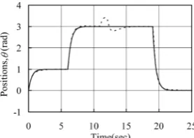
. In simulation, the normal parameters are a= =c 10 and b=1. In the perturbed case, b and c are reducedFigure 1. System output under normal (solid line) and per- turbed case (dashed line).
to 0.5 and 5, respectively, corresponding to doubling of the mass. Moreover, we consider an additive impulse- like disturbance d t
( )
of magnitude 30 acting on the system input between 11 s and 12 s.Figure 1 showed the simulation results under normal (solid line) and perturbed (dashed line) cases. The fol- lowing observations can be made: under normal and per-turbed cases, the optimum response in the whole domain of interest can all be achieved by a set of the same con-trol gains, even under the case that the payload is changed abruptly. This demonstrates that general inte- gral control proposed here has strong robustness, fast convergence and good flexibility, and then can more ef-fectively deal with unknown exogenous disturbances, nonlinearity and uncertainties of dynamics and makes the engineers more easily design a high performance con- troller.
5. Conclusions
Based on the feedback linearization technique, we present a systematic design method for General Integral Control. The main contributions are as follows: 1) A new integral control strategy along with a class of fire-new integrator is proposed; 2) By using the linear system theory and Lyapunov method along with LaSalle’s inva-riance principle, the conditions on the control gains to ensure regionally as well as semi-globally asymptotic stability are provided.
In this paper, only one design method for General Integral Control was presented. It is clear that we cannot expect one particular procedure to apply to all system. Therefore, new design techniques for General Integral Control are needed to solve wider theoretical and prac-tical problems.
REFERENCES
[1] H. K. Khalil, “Universal Integral Controllers for Mini- mum-Phase Nonlinear Systems,” IEEE Transactions on Automatic Control, Vol. 45, No. 3, 2000, pp. 490-494. http://dx.doi.org/10.1109/9.847730
ism Problem for Linear Time-Invariant Multivariable Systems,” IEEE Transactions on Automatic Control, Vol. 21, No. 1, 1976, pp. 25-34.
http://dx.doi.org/10.1109/TAC.1976.1101137
[3] B. A. Francis, “The Linear Multivariable Regulator Prob- lem,” SIAM Journal on Control and Optimization, Vol.15, No. 3, 1977, pp. 486-505.
http://dx.doi.org/10.1137/0315033
[4] A. Isidori and C. I. Byrnes, “Output Regulation of Non- linear Systems,” IEEE Transactions on Automatic Con- trol, Vol. 35, No. 2, 1990, pp. 131-140.
http://dx.doi.org/10.1109/9.45168
[5] H. K. Khalil, “Nonlinear Systems,” Electronics Industry Publishing, Beijing, 2007.
[6] B. S. Liu and B. L. Tian, “General Integral Control,” Pro- ceedings of the International Conference on Advanced Computer Control, Singapore City, 22-24 January 2009, pp. 136-143. http://dx.doi.org/10.1109/ICACC.2009.30
[7] B. S. Liu, and B. L. Tian, “General Integral Control De- sign Based on Linear System Theory,” Proceedings of the 3rd International Conference on Mechanic Automation and Control Engineering, Baotou, Vol. 5, 2012, pp. 3174- 3177.