Munich Personal RePEc Archive
Modeling extreme but plausible losses for
credit risk: a stress testing framework for
the Argentine Financial System
Gutierrez Girault, Matias Alfredo
Banco Central de la Republica Argentina
June 2008
Online at
https://mpra.ub.uni-muenchen.de/16378/
Modeling Extreme but Plausible Losses for Credit Risk
A Stress Testing Framework for the Argentine Financial System
Matías Alfredo Gutiérrez Girault1, Central Bank of Argentina
June 2008
Abstract
While not being widespread, stress tests of credit risk are not new in the Argentine financial system, neither for financial intermediaries nor for the Central Bank. However, they are more often based on rule-of-thumb approaches than on systematic, model based methodologies. The objective of this paper is to fill this gap. With a database that covers the 1994-2006 period we implement a three staged approach. First, we use bank balance sheet data to estimate a dynamic panel data model, with different statistical methodologies, to explain bank losses for credit risk with bank-specific and macroeconomic variables. In a second step, the macroeconomic drivers of bank losses, real GDP growth and cost of short term credit, are modeled with a Vector Autoregression (VAR). The VAR shows the effect of the variables (i.e. risk factors) that we find dominate the domestic business cycle: the price of commodities, the sovereign risk and the federal funds rate. Finally, we use this toolkit to perform deterministic and stochastic scenario analysis. In the first case we use the behavior of the risk factors during the crisis of 1995 (Tequila contagion) and 2001 (Currency Board collapse), and we implement a subjective scenario as well. The stochastic scenarios are performed by Monte Carlo with two alternative methodologies: a non-parametric bootstrapping approach and drawing repeatedly from a multivariate normal distribution. When comparing the estimated unexpected losses to available capital, we find that currently the Argentine financial system is adequately capitalized to absorb the higher losses that would take place in a stress situation.
1
Regulatory Planning and Research Department, Regulation Area, Central Bank of Argentina. I thank
Verónica Balzarotti, Delia Novello, Cristina Pailhé, Patrick Temple and participants at the 5th meeting
of Basel Committee’s Research Task Force Stress Testing Subgroup, held in Paris in October 2007, for their helpful comments and suggestions to an earlier draft. I also want to thank José Rutman for his
support to producing the paper and Angel del Canto for his assistance in preparing part of the data. However, any remaining error is of my sole responsibility. This paper’s findings, interpretations and
I. Introduction
Stress tests of credit risk are increasingly being used as a complement to more standardized and widespread credit risk management tools, such as credit scoring models, segmentation algorithms, rating systems and portfolio credit risk models. While the performance of these methodologies can be fairly stable and reliable under normal business conditions, stress testing methodologies are more appropriate to measure potential credit losses during extreme but plausible adverse events2.
The survey conducted by the Committee on the Global Financial System back in 2004 (CGFS (2005)), in which major banks and securities firms participated, indicated that although most of them performed stress tests for credit risk, these tests were outnumbered by those for market risk: more than 80% of the stress tests reported in the survey were based on trading portfolios, with those based on movements in interest rates being the dominant type. However, the survey also indicated that “In comparison with the previous survey3, there was a greater focus on credit and less attention to equity markets”.
While not being widespread, stress tests of credit risk are not new in the Argentine financial system, neither for financial intermediaries nor for the Central Bank or Argentina (BCRA). During 2006, the Superintendence of Exchange and Financial Institutions conducted a survey (SEFyC (2006)) on stress test practices among local banks. The answers also show the preeminence of market risk over credit risk stress tests: of the 39 institutions in the sample4 30 perform stress tests for interest rate risk and 28 for currency risk, while only 15 stress test credit risk.
Both at financial institutions and at the BCRA stress tests for credit risk are more often based on rule-of-thumb approaches than on systematic, model based methodologies. For example, a usual approach is to simulate a general downgrade of bank borrowers’ creditworthiness, reflected in their risk classification. Since borrowers’ risk classification determines their provision rate, an across the board
migration to lower rating grades implies larger provisions and a stressed income statement. The resulting losses are compared to the available capital. This is for example the approach that the IMF and the World Bank used in the FSAP for Argentina performed in the year 2001.
Part of the interest in this methodology can also be ascribed to the explicit requirement that banks adopting Basel II complement their Pillar I calculations with those resulting from stress tests5 (BCBS (2006)). In addition, it is a relatively unexplored field of research.
2
MAS (2003) advises risk managers “…to adopt a two-pronged approach to risk management, where on the one hand they use various qualitative techniques to measure risk in ordinary business conditions, while on the other, they use stress-tests to quantify likely losses under stress conditions.”
3
See CGFS (2001).
4
Out of 90 institutions contacted, 35 did not perform stress tests and 16 did not answer the survey.
5
Pillar 1, Part 4, Section V, Stress tests used in assessment of capital adequacy, states: “…the
bank must perform a credit risk stress test to assess the effect of certain specific conditions on its IRB regulatory capital requirements (…) For this purpose, the objective is not to require banks to consider
As from 2006, the Central Bank of Argentina is using a non-parametric loan portfolio credit risk model to assess losses in stress scenarios (see Gutierrez Girault (2007)), particularly to the left of the 99.9th percentile of the loss distribution. However, the methodology does not explicitly model the link between the macroeconomic environment and bank losses. The objective of this paper is to fill this gap developing a full fledged methodology to perform stress tests for credit risk, modeling the sources of macroeconomic downturns and the effect on the banking sector.
With a database that covers the 1994-2006 period we implement a three-staged approach. First, we use bank balance sheet data to estimate a dynamic panel data model, with different statistical methodologies, to explain bank losses for credit risk with bank-specific and macroeconomic variables. In a second step, the macroeconomic drivers of bank losses, real GDP growth and cost of short term credit are modeled with a Vector Autoregression (VAR). The VAR shows the effect of the variables (i.e. risk factors) that we find dominate the domestic business cycle: the price of commodities, the sovereign risk and the federal funds rate. Finally, we use this toolkit to perform deterministic and stochastic scenario analysis. In the first case we use the behavior of the risk factors during the crisis of 1995 (Tequila contagion) and 2001 (Currency Board collapse), and we implement a subjective scenario as well. The stochastic scenarios are performed by Monte Carlo with two alternative methodologies: a non-parametric bootstrapping approach and drawing repeatedly from a multivariate normal distribution. The rest of the paper is organized as follows. Section II describes the data used, while section III estimates the models. Section IV performs the scenario analysis, comparing the estimated unexpected losses to the available capital. Section V contains the conclusions.
II. Data
To construct the stress test framework we use a database with annual data that covers the thirteen year period comprised between 1994 and 2006. The reason for choosing it is the availability of bank balance sheet data: the information previous to November 1994 is not incorporated to the BCRA’s digital information systems (being
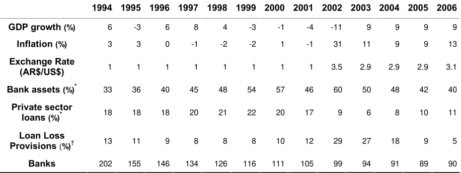
stored in paper format). Besides, it encompasses years of high and moderate growth, as well as economic downturns and a sharp recession. Since during this period new banks initiated their operations, while others merged or closed, we have an unbalanced panel which contains information for at most 13 years for a number of banks that range from 202 in 1994 to 90 in 2006. Table 1 characterizes the banking system throughout this period.
Specific issues to be addressed under the supervisory review process, states in section B, Credit Risk: “1. Stress tests under the IRB approaches. A bank should ensure that it has sufficient capital to meet the Pillar 1 requirements and the results (where a deficiency has been indicated) of the credit risk stress test performed as part of the Pillar 1 IRB minimum requirements… The results of the
Table I. Summary macroeconomic and banking statistics (1994 – 2006)
1994 1995 1996 1997 1998 1999 2000 2001 2002 2003 2004 2005 2006
GDP growth (%) 6 -3 6 8 4 -3 -1 -4 -11 9 9 9 9
Inflation (%) 3 3 0 -1 -2 -2 1 -1 31 11 9 9 13
Exchange Rate
(AR$/US$) 1 1 1 1 1 1 1 1 3.5 2.9 2.9 2.9 3.1
Bank assets (%)* 33 36 40 45 48 54 57 46 60 50 48 42 40
Private sector
loans (%)* 18 18 18 20 21 22 20 17 9 6 8 10 11
Loan Loss
Provisions (%)† 13 11 9 8 8 8 10 12 29 27 18 9 5
Banks 202 155 146 134 126 116 111 105 99 94 91 89 90
*
Expressed as fraction of GDP.†Loan loss provisions expressed as fraction of loans to the non-financial private sector.
In our estimations the bank loss rate for credit risk is proxied by the ratio of loan loss provisions (LLPs) to loans to the private sector6. According to the provisioning regulation set forth by the BCRA, provisions for credit risk depend on the risk rating of the bank borrowers. Following detailed guidelines set by the BCRA, risk ratings are assigned to the borrowers by each of their corresponding creditors7 and range between 1 and 5 depending on the perceived risk. In the case of retail borrowers, the risk classification depends on their payment behavior, in particular of the days past due, with borrowers less than 90 days past due being classified 1 or 2. For commercial borrowers the relationship between days in arrears and the risk classification is less direct; there are criteria in addition to payment behavior to decide how the firm will be classified, such as the projected cash-flow, business sector, etc.
The first downturn included in the sample took place during 1995, when the Argentine economy suffered the consequences of the end-of-1994 Mexican devaluation. As a result of the contagion (the so-called Tequila effect) real GDP fell by 2.8% in 1995; nevertheless, the recession was short-lived and in 1996 the Argentine economy was growing fast again.
The 2002 crisis was far more complex. Its origin can be traced back to the second half of 1997, when emerging markets were hit hard in the aftermath of the crisis in South East Asia. Confidence regarding emerging market resilience faltered further during the Russian crisis in the second half of 1998, and after Brazil’s currency crisis
and abandonment of its crawling peg in January 1999. In addition to this international adverse juncture, throughout all this period Argentina showed a weak fiscal position, therefore being particularly vulnerable to the changing mood in international financial markets and displaying a negative debt dynamic. The 1998–2001 period also showed a hostile international environment in the real sector, with weak commodity prices and an overvalued domestic currency.
6 In the computation of this ratio we include on-balance loans and provisions only. Therefore, loans
completely written-off and removed to off-balance accounts have not been included in the computation of the LLPs ratio.
7 This implies that individuals with operations with many banks receive one risk classification from
The perception that the Currency Board and the servicing of the public debt were unsustainable, and that the government lacked the necessary political strength to push forward the required reforms gained momentum in the third quarter of 2001, when the bank run which had been incipient as from the beginning of that year became massive. At the end of November the financial system collapsed and the conversion of banks’ deposits was suspended: on November 30 the government
declared a deposit freeze. By February 2002 the government had abandoned the Currency Board, defaulted on the public debt and converted to local currency most of the obligations set in US dollars, including bank deposits in that currency8. That year, real GDP fell by 11%.
The behavior of the Argentine economy in the estimation window, summarized by GDP growth, consumer price index (CPI) inflation and the exchange rate, is depicted in Graph 1.
Graph 1. Growth, inflation and exchange rate (1994 – 2006)
0,0 0,5 1,0 1,5 2,0 2,5 3,0 3,5 4,0
1994 1995 1996 1997 1998 1999 2000 2001 2002 2003 2004 2005 2006
A
R
$
/U
S
$
-15% -10% -5% 0% 5% 10% 15% 20% 25% 30% 35%
exchange rate - left axis inflation rate - right axis GDP growth - right axis
Graph 2 shows GDP growth and the bank loss rate for credit risk in the estimation
window. It is evident how the financial turmoil that began in 1997 impacted the local business cycle, after which the Argentine economy slipped into the recession that concluded in the 2002 crisis. It also shows the clear inverse and strong relationship between GDP growth and the ratio of LLPs to loans to the private sector.
8 Bank deposits in US$ were converted to pesos at an exchange rate (AR$/US$) lower than the one
Graph 2. LLPs and GDP Growth (1994 – 2006)
-15% -10% -5% 0% 5% 10% 15% 20% 25% 30%
1994 1995 1996 1997 1998 1999 2000 2001 2002 2003 2004 2005 2006
GDP growth LLPs (% of Loans)
III. Methodology9
This section describes the methodology developed to perform macro stress testing of credit risk. In the first part we present the micro or credit risk “satellite” model, which
links the macroeconomic variables to bank losses. Secondly we present the macroeconomic model, used to link external shocks to the macroeconomic variables that are relevant to explain bank losses for credit risk.
III.a. The Microeconomic or Credit Risk “Satellite” Model
To construct our measure of loss for credit risk we use the ratio of LLPs to loans to the private sector, subject to a logit transformation10. The simplest approach to estimate our panel data model would be with the static fixed-effects estimator, the latter being a reasonable assumption since we are working with all the financial institutions in the financial system. The equation to be estimated would be,
it t it i
it =á +Xâ+Zù+å
y (1)
where yit is the dependent variable (loss rate) for bank i in period t, ái represents firm specific and time invariant (fixed) effects (unobserved heterogeneity), Xit contains bank-specific time varying variables (observed heterogeneity) and a constant, Zt has time varying macro variables, common to all the banks and åit is the bank-specific disturbance in period t. There is a single covariate included in X, which is the lagged first difference in bank loan growth, which measures to what extent the bank has been speeding up (or slowing down) its lending activity. Time varying macro
variables, contained in Z, include current GDP growth, the lagged overdraft interest rate (in AR$) and an interaction effect between the lagged GDP growth and lagged interest rate.
However, a visual inspection of the time pattern of the pooled loss rate (Graph 2) suggests that the dependent variable would be better modeled with a dynamic specification. This can be accomplished introducing the lagged dependent variable as a regressor in the static fixed-effects model. This dynamic fixed-effect or least squares dummy variable (LSDV) estimator poses the following model,
it t it i 1 -it
it =ñy á +X â+Zù+å
y (2)
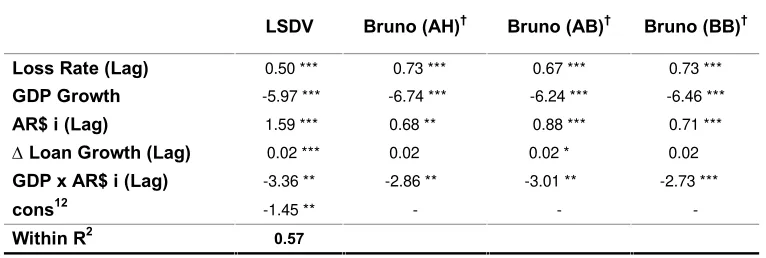
[image:8.595.106.489.442.571.2]which is estimated by applying OLS to the model expressed in deviations from time means. The estimated coefficients are shown in Table 2. However, it is well known that this approach renders biased estimates: the LSDV estimator is inconsistent for finite T and N11 (Nickell (1981)), which is in fact the case of our sample panel. The reason for this bias is the correlation between the transformed lagged dependent variable and the transformed current disturbance. In an attempt to cope with this bias, Kiviet (1995) tries to correct the LSDV estimates by subtracting from them an approximation of their small sample bias. However, this approach does not handle unbalanced panels. Bruno (2004) develops a two-step procedure for correcting the LSDV bias in unbalanced panels, which in the first step uses consistent estimates of the equation coefficients. The estimated coefficients computed with the estimator presented in Bruno (2004), LSDVC, are also shown in Table 2.
Table 2. Micro model: LSDV and LSDV-corrected dynamic specifications
LSDV Bruno (AH)† Bruno (AB)† Bruno (BB)†
Loss Rate (Lag) 0.50 *** 0.73 *** 0.67 *** 0.73 ***
GDP Growth -5.97 *** -6.74 *** -6.24 *** -6.46 ***
AR$ i (Lag) 1.59 *** 0.68 ** 0.88 *** 0.71 ***
Loan Growth (Lag) 0.02 *** 0.02 0.02 * 0.02
GDP x AR$ i (Lag) -3.36 ** -2.86 ** -3.01 ** -2.73 ***
cons12 -1.45 ** - - -
Within R2 0.57
Note: ***, ** and * indicate statistical significance at 99%, 95% and 90% confidence levels. †Significance tests were computed with bootstrapped standard errors. First step estimates were obtained from the Anderson – Hsiao, Arellano – Bond and Blundell – Bond consistent estimators respectively.
Anderson and Hsiao (1982) propose an instrumental-variable estimator (AH) which is consistent for T fixed and N, and therefore is also suitable given the characteristics of our sample. This estimator is based on a differenced form of the original dynamic equation,
1 -it it 1 -t t 1
-it it 2 -it 1 -it 1 -it
it -y = y - y +X â-X â+ Z - Z +
-y ñ ñ ù ù å å (3)
11 Behr (2003) shows that the asymptotic bias of the LSDV estimated coefficients is increasing in
, in the number of individuals in the sample (N) and in the sum of squared residuals, and decreasing in T. Judson and Owen (1996) show that the bias of the estimate is more severe than that of .
(
it-1 it-2) (
it it-1)
(
t t-1)
it it-1 1-it
it -y = y -y +â X -X + Z -Z +
-y ñ ù å å (4)
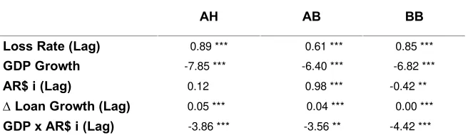
which cancels out the fixed effects, that may be correlated with the exogenous variables. Since the difference of the lagged endogenous variable is correlated with the difference in the error term, Anderson and Hsiao (1982) suggest instrumenting (yit-1 – yit-2) with yit-2 or (yit-2 – yit-3), which are expected to be uncorrelated with the differenced error term. The estimated coefficients of the AH estimator13 are included in Table 3.
[image:9.595.135.463.416.511.2]Although N-consistent, the AH estimator is not efficient since it does not use all the available moment conditions. Arellano and Bond (1991) propose a Generalized Method of Moments (GMM) estimator (AB), which also first-differences the SE model but obtains additional instruments from orthogonality conditions between the lagged values of yit and (it-it-1). However, Blundell and Bond (1998) show that when is moderately large and T is moderately small, the AB estimates have large finite sample bias and poor precision. Therefore, we also compute the System GMM estimator, developed in Blundell and Bond (1998), who exploit further moment conditions. The System GMM estimator is however not free from problems; for example Hayakawa (2005) shows that when the variances of the individual effects and of the disturbances are unequal the bias of this estimator is fairly large. The estimates obtained from both GMM based approaches, AB and BB, are also included in Table 3.
Table 3. Micro model: IV and GMM based dynamic specifications
AH AB BB
Loss Rate (Lag) 0.89 *** 0.61 *** 0.85 ***
GDP Growth -7.85 *** -6.40 *** -6.82 ***
AR$ i (Lag) 0.12 0.98 *** -0.42 **
Loan Growth (Lag) 0.05 *** 0.04 *** 0.00 ***
GDP x AR$ i (Lag) -3.86 *** -3.56 ** -4.42 ***
Note: ***, ** and * indicate statistical significance at 99%, 95% and 90% confidence levels.
In spite of the differences in the statistical methodologies used, in general all estimated coefficients have the expected signs. The high coefficient of the autoregressive component reflects the persistence of the loss rate and supports our initial guess based on the observation of Graph 2. The estimated effects of the macroeconomic variables are also intuitive: higher GDP growth lowers bank losses since it improves the credit quality of bank borrowers, while the converse happens with higher interest rates. The estimate for bank credit granting stance14 indicates that those banks that were lending aggressively are likely to experience larger losses.
Given the abovementioned advantages and disadvantages of the diverse dynamic panel data estimators, the features of our sample panel (unbalanced with large N and short T) and the fact that the autoregressive component seems to be large, the scenario analysis of section IV will be performed with the estimators developed in
13 We instrument (y
it-1– yit-2) with yit-2. 14
Bruno (2004) and Blundell and Bond (1998). However, since the latter yields a negative estimated coefficient for the lagged interest rate, implying that higher interest rates yield lower losses for credit risk, the conclusions drawn from this estimator must be interpreted with prudence.
III.b. The Macroeconomic Model
The approach used to modeling the macroeconomic variables that explain the behavior of bank losses is non-structural. With a vector autoregression (VAR), we estimate the following system:
t t p -t p 2
-t 2 1 -t 1
t =A Y +A Y + A Y +BX +å
Y (5)
where Yt is a k vector of endogenous variables, Xt a vector of exogenous variables, A1,A2 … Ap and B are matrices of coefficients to be estimated, and åt is a vector of innovations that may be contemporaneously correlated but are uncorrelated with their own lagged values and the right-hand side variables.
The endogenous variables included in vector Y are real GDP growth and AR$ interest rate for overdrafts, while the strictly exogenous variables in Xt are sovereign risk, the federal funds rate15 and the price of commodities. Sovereign risk is measured by the EMBI index for Argentina for the years between 1994 and 2002; as from 2003 it is measured by the spread of the BODEN 2012 US$ bond over US Treasury bonds of similar modified duration. The fed funds rate has nearly perfect correlation with the yield of US Treasury bonds, in particular with short-maturity ones, and in practice it sets the floor to the cost at which an emerging economy government can obtain financing in the international capital market. Finally, the price of commodities is measured by an index expressed in US dollars and published by the BCRA.
The usual lag-order selection statistics (Final Prediction Error, Akaike’s Information
Criterion, Schwarz's Bayesian information criterion (SBIC) and the Hannan and Quinn information criterion (HQIC)) as well as other preliminary exploratory analysis suggest a one period lag structure be used. Therefore in equation (5) p equals 1 and the VAR estimated is,
t t 1 -t 1
t =A Y +BX +å
Y (6)
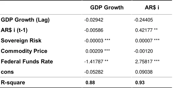
According to the Lagrange-Multiplier Test there is neither first nor second order autocorrelation in the residuals. All the eigenvalues associated to the stability test lie inside the unit circle; therefore, the estimated VAR satisfies the stability condition. The estimated coefficients for equation (6) are shown in Table 4.
15 The interest rate at which depository institutions lend balances at the Federal Reserve to other
Table 4. Macro model: Vector Autoregression
GDP Growth AR$ i
GDP Growth (Lag) -0.02942 -0.24405
AR$ i (t-1) -0.00586 0.42177 **
Sovereign Risk -0.00003 *** 0.00007 ***
Commodity Price 0.00209 *** -0.00120
Federal Funds Rate -1.41787 ** 2.75817 ***
cons -0.05282 0.09038
R-square 0.88 0.93
Note: *, ** and *** indicate statistical significance at 99%, 99.5% and 99.9%
confidence levels.
Simple as it is, this reduced form VAR renders estimated coefficients with the expected signs: lagged domestic interest rates impact negatively on the GDP growth rate, the sovereign risk impacts positively on domestic interest rates and negatively on economic growth, an increase in the federal funds rate also raises domestic interest rates and lowers growth and finally, better (higher) prices in commodities fuel growth.
Our estimated macroeconomic model reflects the basic dynamic features of the Argentine business cycle. The federal funds rate proxies the degree of international liquidity and sets a floor to the cost for the government of borrowing from the international capital market. The sovereign risk measures the mood of local and international investors towards Argentina and is strongly correlated with the capital flows that expand and contract aggregate demand. Finally, the commodity price index indicates the direction of the income effect due to changes in the price of local exports. However, this model fails to take into account other effects that may be important to explain the business cycle. In particular, we are modeling first round effects only, i.e., the effect of external shocks on the macroeconomy and ultimately on the banking sector’s credit losses. Marcucci and Quagliariello (2005) incorporate
to their VAR the feedback effect that a stress situation in the banking sector has on the business cycle, amplifying the effect of the original shocks, via the bank capital channel.
IV. Scenario Analysis
In this section we stress test the losses for credit risk of the banking sector. To this purpose we use the toolkit developed in the previous section, together with different approaches to incorporating shocks in the risk factors that drive the business cycle. Our stress tests take place during 2007: they simulate the behavior of the bank loss rate as a result of an extreme but plausible adverse scenario taking place during that year.
sovereign default of 2002. We also simulate a judgmental or subjective scenario, assuming a deterioration of all risk factors with respect to their position as of 2006.
In the second and third approaches the scenario analysis are stochastic and obtained by Monte Carlo simulation. In one case we implement a bootstrapping technique, while in the other we sample repeatedly from a multivariate normal distribution to obtain correlated realizations of the risk factors.
Regardless of how the risk factors are assumed to behave or simulated, we then use the macroeconomic VAR to forecast GDP growth and AR$ interest rates, and our “satellite” model to estimate bank losses for credit risk during 2007. To assess the
reliability of our results we will estimate the ratio of LLPs with two models: Blundell and Bond’s (1998) System GMM estimator (BB) and Bruno’s (2004) LSDV corrected
estimator with first step System GMM estimates (Bruno (BB)).
Having estimated the ratio of LLPs to loans to the private sector with both dynamic panel data methodologies, we quantify the capital needed to cover the unexpected losses for credit risk. In the deterministic scenario they are computed as the difference between the estimated LLPs for 2007, in the stress scenario, and LLPs as of end 2006, both as a fraction of loans to the private sector. In the stochastic scenario analysis, unexpected losses at the 99.9th confidence level are computed as the 99.9th percentile of the simulated distribution, net of prevailing provisions.
Both in the deterministic and stochastic tests, the banking sector as a whole needs to have enough capital to absorb the increase in the ratio of LLPs that would result from the stress event. Taking Tier 1 and Tier 2 capital as of end 2006 and subtracting from it regulatory capital requirements for interest rate risk (market risk in the banking book), the remaining available capital covered up to 30.3% of the loans to the private sector.
IV.a. Deterministic Scenarios
Historical Scenario Analysis
In this simple approach to stress tests we will first evaluate the macroeconomic model developed in section III.b. with the realizations of the risk factors observed after the Mexican devaluation and during the Argentine Currency Board collapse. In the second case we perform a two-year analysis: the crisis began in 2001 with a loss of confidence that resulted in massive capital outflows and a bank panic by the end of that year. In 2002, the sovereign default and abandonment of the Currency Board deepened the crisis. Table 5 shows, for each historical episode, the risk factors and the observed GDP growth, AR$ interest rates and the ratio of LLPs to loans to the private sector.
For each scenario the results obtained from the macroeconomic model are introduced into the microeconomic or “satellite” model to forecast the losses for credit
Table 5. Description of Historical Scenarios
Risk Factors Macroeconomic Variables
Sovereign Risk (b.p.)
Commodities Price
Index† Fed Funds Rate (%) GDP Growth (%) AR$ Interest Rate (%)
LLPs/L (%)
Scenario I. Contagion from Tequila Crisis
1995 1159.9 91.6 5.8 -2.8 41.6 10.6
Scenario II. Currency Board Crisis
2001 1544.3 70.4 3.9 -4.4 40.4 12.4
2002 5726.3 74.4 1.7 -10.9 63.2 28.8
†
December 1995 = 100.
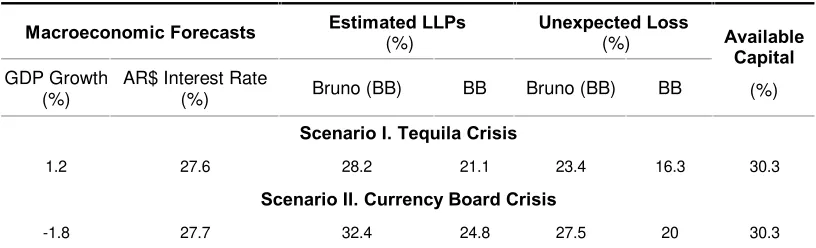
For the same realizations of the risk factors observed during the abovementioned events, Table 6 includes the forecasted GDP growth and AR$ interest rates, obtained from the macroeconomic model.
Table 6. Historical Scenario Analysis - Results
Macroeconomic Forecasts Estimated LLPs
(%)
Unexpected Loss (%)
GDP Growth (%)
AR$ Interest Rate
(%) Bruno (BB) BB Bruno (BB) BB
Available Capital
(%)
Scenario I. Tequila Crisis
1.2 27.6 28.2 21.1 23.4 16.3 30.3
Scenario II. Currency Board Crisis
-1.8 27.7 32.4 24.8 27.5 20 30.3
†
Expressed as fraction of loans to the non-financial private sector.
During 2006 the environment was particularly favorable from the point of view of sovereign risk (364 b.p.), the fed funds rate (5%) and the price of commodities (105.7). Therefore, scenarios I (Tequila) and II (Currency Board crisis) imply an increase in sovereign risk of 219% and 324% respectively, and a reduction in the price of commodities of 13.4% and 33.4%. The fed funds rate was 16% higher in 1995 but 22% lower in 2001. Although we evaluate the models with the same risk factors as observed in the chosen events, the forecasted GDP and AR$ interest rates should be different from the ones observed on those occasions, since the macroeconomic conditions prevailing in 2006 are significantly different from those in 1994 and 2000, before the shocks took place.
[image:13.595.93.501.333.457.2]However, the event that motivates the second scenario lasted up to 2002, as shown in Table 5. Although the risk factors affected the country negatively in 2001, the economy slipped into a massive crisis in the first half of 2002, after the overshooting (almost 300% depreciation) of the exchange rate and debt default. If we reproduce the exercise with the risk factors observed in 2002 (sovereign risk at 5726.3 b.p., fed funds rate at 1.7% and the commodities index at 74.4), the panel data models yield a LLPs/L ratio that ranges between 62% and 50%. Although in this case available bank capital would not suffice to cover these higher losses, it is actually not expected to cover them either: bank losses in worst-case scenarios can not be completely absorbed by bank capital. The year 2002 saw a major and massive disruption in economic activity take place, particularly in the banking system. The AR Peso depreciated almost 300% in the first quarter, the public debt was defaulted and bank deposit convertibility was suspended. Since most bank loans and deposits were in US$ they were converted to AR$ at an exchange rate that partially liquefied them. In such a worst-case scenario taking place bank capital, high as it may be, can hardly cope with the unexpected losses that arise, which require public policies of a different kind to deal with them.
Even though Table 6 leads to the conclusion that current bank capital is sufficient to absorb bank losses, the results are conservative, and therefore overestimate losses, for at least the following reasons. Firstly, the model does not incorporate any reaction function from bank managers or the central bank to lessen the intensity of the adverse scenario. Secondly, and perhaps more importantly, given the observed behavior of the risk factors it seems highly unlikely that during the course of only one year they will deteriorate as assumed in the scenarios. Back in the Tequila and Currency Board crisis the sovereign risk averaged 600 and 670 b.p. before increasing to 1160 b.p. and 1544 b.p. respectively. In the case of the commodity price index, while its past behavior supports the possibility of a 13.4% reduction (to the Tequila crisis level), the possibility that it might fall 33.4% in the course of a year is remote. Therefore, these results can perhaps be evaluated as taking place during the course of two years, which would give bank managers more leeway to mitigate losses and to inject capital.
Judgmental Scenario Analysis
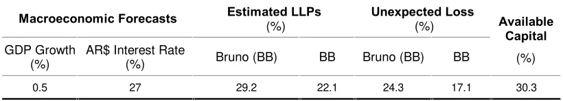
[image:14.595.92.502.678.752.2]While the historical scenarios have the advantage that they represent situations that have happened in the past, they do on the other hand run the risk of being obsolete or inadequate given the current juncture. Therefore in what follows we define a scenario for 2007 subjectively, assuming: a 150% increase in sovereign risk to 900 b.p., a 20% reduction in the commodity price index to 85 and a 20% increase in the fed funds rate to 6%. Table 7 shows the forecasted GDP and interest rates for 2007 and the stressed losses.
Table 7. Judgmental Scenario Analysis – Results
Macroeconomic Forecasts Estimated LLPs
(%)
Unexpected Loss (%)
GDP Growth (%)
AR$ Interest Rate
(%) Bruno (BB) BB Bruno (BB) BB
Available Capital
(%)
0.5 27 29.2 22.1 24.3 17.1 30.3
†
The results, on this occasion stemming from a subjective scenario, indicate the resilience of the Argentine banking sector to extreme but plausible adverse shocks. The estimated unexpected losses that would have happened during 2007 had this scenario taken place range between 17.1% and 24.3% with the BB and Bruno (BB) estimators, and are below the capital available in the banking system to cover unexpected credit risk.
IV.b. Stochastic Scenario Analysis
Bootstrapping Approach
In this sub-section we implement a non-parametric approach to obtaining a distribution for the ratio of LLPs to loans to the private sector, by performing Monte Carlo simulation from the risk factors’ bootstrapped joint distribution. First we
estimate the joint distribution of the risk factors in the VAR by means of a multivariate or parallel bootstrapping. This is done by randomly resampling from the risk factors’ empirical joint distribution: we take their historical monthly time series between 1993 and 2007 and draw 50,000 samples of 12 observations with replacement16. Each draw contains a realization for each risk factor, the three of them corresponding to the same month. By this means we attempt to preserve the multivariate properties of the risk factors, particularly their structure of correlations. Then each risk factor’s 12
observations in each sample are averaged, where the three averages constitute a simulated annual realization from the risk factors’ bootstrapped joint distribution. The
bootstrapped marginal density of the sovereign risk is shown in Graph 3.
Graph 3. Sovereign Risk Bootstrapped Marginal Density
0,0% 0,5% 1,0% 1,5% 2,0% 2,5% 3,0% 3,5% 4,0% 4,5% 3 9 0 4 4 0 4 9 0 5 4 0 5 9 0 6 4 0 6 9 0 7 4 0 7 9 0 8 4 0 8 9 0 9 4 0 9 9 0 1 0 4 0 1 0 9 0 1 1 4 0 1 1 9 0 1 2 4 0 1 2 9 0 1 3 4 0 1 3 9 0 1 4 4 0 1 4 9 0 1 5 4 0 1 5 9 0 1 6 4 0 1 6 9 0 1 7 4 0 1 7 9 0
Sovereign Risk (b.p.)
16 The risk factors
’ behavior during 2002 was not included in any of the stochastic stress tests, since
With the three bootstrapped marginals and the macro model we compute one-step ahead forecasts of the macroeconomic variables. By doing this with each “observation” of the distribution we simulate 50,000 forecasts of both GDP growth and domestic interest rates. Finally, the simulated GDP growth distribution is used to compute the distribution of banks’ ratio of LLPs by means of the dynamic panel data
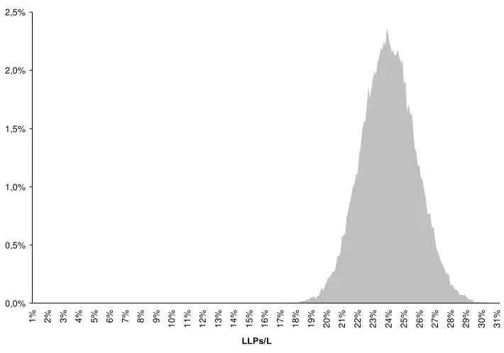
[image:16.595.120.475.307.556.2]models. The results for the selected approaches are shown in Table 8, and the loss distribution obtained from the Bruno (BB) model is shown in Graph 4.
Table 8. Stochastic Scenario Analysis – Bootstrapped Loss Distribution†
Minimum Median Mean 99,9% Unexpected
Loss
Available Capital
Bruno (BB) 16.4 24 24 29.4 24.5 30.3
BB 11.4 17.5 17.5 22.1 17.3 30.3
†
All figures are expressed as percentage of loans to the non-financial private sector.
Graph 4. Bootstrapped Loss Distribution
0,0% 0,5% 1,0% 1,5% 2,0% 2,5% 1
% 2% 3% 4% %5 6% 7% 8% 9%
1 0 % 1 1 % 1 2 % 1 3 % 1 4 % 1 5 % 1 6 % 1 7 % 1 8 % 1 9 % 2 0 % 2 1 % 2 2 % 2 3 % 2 4 % 2 5 % 2 6 % 2 7 % 2 8 % 2 9 % 3 0 % 3 1 % LLPs/L
Having computed the Value-at-Risk corresponding to a 99.9% confidence level, we subtract the ratio of LLPs as of end 2006. The result is the potential downside credit risk that would result from an adverse scenario produced by the combination of the risk factors, with a 99.9% confidence level. The results in Table 8 show that the estimated unexpected losses range from 17.3% with the BB estimator to 24.5% with the Bruno (BB) estimator, which are similar to those obtained in the deterministic stress tests. It also shows that these unexpected losses can be covered with available capital, no matter what “satellite” model is chosen to estimate LLPs.
simulating annual risk factors from monthly data we attempt to tackle the first limitation of this approach, since the underlying sample from which we bootstrap contains 159 observations. However, by sampling at random from monthly data we may indeed be disrupting any possibly existing relevant time pattern in data.
Multivariate Normal Approach
As an alternative to the non-parametric analysis developed above, we estimate a credit loss distribution by performing Monte Carlo from a multivariate normal distribution. To that purpose we take 50,000 random draws from a standard multivariate normal distribution, which are then transformed into correlated shocks using a Cholesky decomposition of risk factors’ covariance matrix. Having then
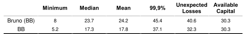
[image:17.595.95.495.327.383.2]simulated 50,000 correlated realizations of the risk factors, we forecast 50,000 realizations of GDP growth. These are used to obtain LLPs estimates with the Bruno (BB) and BB microeconomic models. The results are summarized in Table 9 and the loss distribution obtained with the Bruno (BB) estimator is shown in Graph 5.
Table 9. Stochastic Scenario Analysis – Multivariate Normal Loss Distribution†
Minimum Median Mean 99,9% Unexpected
Losses
Available Capital
Bruno (BB) 8 23.7 24.2 45.4 40.6 30.3
BB 5.2 17.3 17.8 37.1 32.3 30.3
†
All figures are expressed as percentage of loans to the non-financial private sector.
According to this Monte Carlo experiment and with a 99.9% confidence level, banks unexpected losses would escalate to a range between 32.3% to 40.6% of the loans to the private sector. The 32.3% floor corresponds to the BB estimator, whose potential problems (particularly as a result of a negative estimated coefficient in the lagged interest rate) were discussed in section III.a. On the other hand, unexpected losses derived from the Bruno (BB) estimator would not be completely covered with bank capital. These estimated unexpected losses are not only very different to those obtained with the other deterministic and stochastic methodologies, but also are inconsistent with the observed ratio of LLPs, which in the estimation window never exceeded 29%.
The reliability of these results is affected by our assumption regarding the multivariate normal nature of risk factors, which implies Gaussian marginal for the risk factors and that for the sovereign risk is unrealistic. Also, the simulated risk factors’ marginals display a range of variation inconsistent with the one observed in
Graph 5.Multivariate Normal Loss Distribution 0,0% 0,1% 0,2% 0,3% 0,4% 0,5% 0,6% 0,7% 0,8% 0,9% 1
% 3% 5% 7% 8%
1 0 % 1 2 % 1 4 % 1 6 % 1 7 % 1 9 % 2 1 % 2 3 % 2 5 % 2 6 % 2 8 % 3 0 % 3 2 % 3 4 % 3 5 % 3 7 % 3 9 % 4 1 % 4 3 % 4 4 % 4 6 % 4 8 % 5 0 % 5 2 % 5 3 % 5 5 % LLPs/L V. Conclusions
Stress tests for credit risk have evolved in the last years as an important element in bank risk management. Throughout this paper we attempted to construct a full fledged methodology for performing macro stress testing for credit risk. To this end we developed the different elements of the methodology. With panel data techniques we estimated a dynamic model for bank losses for credit risk. Although we compared the estimated coefficients with different statistical approaches, in almost all cases they had the expected sign. The macroeconomic variables that are covariates in the “satellite” model were modeled with a Vector Autoregression that forecasts GDP
growth and interest rates with the sovereign risk, the price of commodities and the federal funds rate.
To model credit risk losses in stress situations we followed different approaches: deterministic (historical and judgmental) and stochastic with Monte Carlo simulation (based on bootstrapping and in the multivariate normal distribution). The historical scenarios have the advantage that they reproduce events experienced by the Argentine economy, while the judgmental scenario is perhaps more informative of what would happen should the current juncture (as of end 2006) deteriorate. On the other hand, the judgmental scenario does not necessarily incorporate the covariances between risk factors and might therefore be excessively conservative. Stochastic scenarios have the advantage that they yield a loss distribution and allow calculation of loss rates with different confidence levels. However, the results rely heavily on the ability of the approach to replicate the multivariate nature of the risk factors.
the stress tests yield unexpected losses that range between 16% and 28% of loans to the private sector, below available bank capital.
The conclusions in this paper about bank solvency in stress scenarios did not address the degree of capital adequacy at a bank level, since unexpected losses have been compared to the capital ratio of the banking sector as a whole. Other pending topics that may be addressed in future research include modeling risk factors dependence structure using other techniques, such as with copula functions or with a multivariate extreme value theory approach.
Finally, it is of paramount importance that the results herein obtained regarding credit risk losses in stress scenarios are modeled jointly with other major risks to the financial system, such as interest rate risk or liquidity risk. This would enable assessment of the overall capacity of the banking sector to absorb unexpected losses of various risks arising in stress scenarios.
References
Arellano, M. and S. Bond (1991). Some Tests of Specification for Panel Data: Monte Carlo Evidence and an Application to Employment Equations, Review of Economic Studies, 58, 277-297.
Anderson, T.W. and C. Hsiao (1982). Formulation and Estimation of Dynamic Models using Panel Data, Journal of Econometrics, 18, 47-82.
Basel Committee on Banking Supervision (2006). International Convergence of Capital Measurement and Capital Standards: A Revised Framework - Comprehensive Version, Bank for International Settlements.
Behr, A. (2003). A comparison of dynamic panel data estimators: Monte Carlo evidence and an application to the investment function. Discussion Paper 05/03, Deutsche Bundesbank.
Blundell, R. and S. Bond (1998). Initial Conditions and Moment Restrictions in Dynamic Panel Data Models, Journal of Econometrics, 87, 115-143.
Bruno, G.S.F. (2004). Approximating the Bias of the LSDV Estimator for Dynamic Unbalanced Panel Data Models, Universita Bocconi, Instituto di Economia Politica.
Committee on the Global Financial System (2001). A survey of stress tests and current practice at major financial institutions, Bank for International Settlements.
Committee on the Global Financial System (2005). Stress testing at major financial institutions: survey results and practice, Bank for International Settlements.
Hayakawa, H. (2005). Small Sample Bias Properties of the System GMM Estimator in Dynamic Panel Data Models, Discussion Paper Series N°82, Institute of Economic
Research, Hitotsubashi University.
Jorion, P. (2001). Value at Risk, McGraw-Hill.
Judson, R.A. and A.L. Owen (1996). Estimating Dynamic Panel Data Models: A Practical Guide for Macroeconomists. Federal Reserve Board of Governors.
Kiviet, J.F. (1995). On bias, inconsistency and efficiency of various estimators in dynamic panel data models, Journal of Econometrics, 68, 53-78.
Marcucci, J. and M. Quagliariello (2005). Is Bank Portfolio Procyclical? Evidence from Italy using a Vector Autoregression. Discussion Paper in Economics 2005/09, The University of York.
Monetary Authority of Singapore (2003). Technical Paper on Credit Stress-Testing, MAS Information Paper 01-2003.
Nickell, S. (1981). Biases in Dynamic Models with Fixed Effects, Econometrica, Vol. 49, No. 6. pp. 1417-1426.