Inequality and development: Evidence from semiparametric estimation with panel data

Munich Personal RePEc Archive

Inequality and development: Evidence

from semiparametric estimation with

panel data

Zhou, X. and Li, Kui-Wai

City University of Hong Kong

December 2011

Online at

https://mpra.ub.uni-muenchen.de/36418/

Our reference: ECOLET 4915

P-authorquery-v8

AUTHOR QUERY FORM

Journal:

Economics Letters

Article Number:

4915

Please e-mail or fax your responses and any corrections to:

E-mail: [email protected]

Fax: +44 1392 285879

Dear Author,

Please check your proof carefully and mark all corrections at the appropriate place in the proof (e.g., by using on-screen annotation in

the PDF file) or compile them in a separate list.

For correction or revision of any artwork, please consult

http://www.elsevier.com/artworkinstructions

.

Any queries or remarks that have arisen during the processing of your manuscript are listed below and highlighted by flags in the

proof. Click on the

‘Q’

link to go to the location in the proof.

Location

in article

Query / remark

click on the Q link to go

Please insert your reply or correction at the corresponding line in the proof

Q1

Uncited references: This section comprises references that occur in the reference list but not in the body of the

text. Please cite each reference in the text or, alternatively, delete it. Any reference not dealt with will be retained

in this section.

Thank you for your assistance.

Highlights

◮Nonparametric and semiparametric models on Kuznet’s equality-development relationship.◮Sample of 75 countries for the period 1962–2003.◮

∧

Economics Letters xx (xxxx) xxx–xxx

Contents lists available atScienceDirect

Economics Letters

journal homepage:www.elsevier.com/locate/ecolet

Inequality and development: Evidence from semiparametric estimation with

panel data

Xianbo Zhou

a

, Kui-Wai Li

b,∗

a_{Lingnan College, Sun Yat-sen University, China} b_{City University of Hong Kong, Hong Kong}

a r t i c l e i n f o

Article history:

Received 17 August 2010 Received in revised form 12 July 2011

Accepted 14 July 2011 Available online xxxx

JEL classification:

C14 O1

Keywords:

Kuznet’s inverted-U Semiparametric model Unbalanced panel data

a b s t r a c t

Evidences from nonparametric and semiparametric unbalanced panel data models with fixed effects show that Kuznet’s inverted-U relationship is confirmed when economic development reaches a threshold. The model tests justify semiparametric specification. The integrated net contribution of control variables to inequality reduction is significant.

©2011 Elsevier B.V. All rights reserved.

1. Introduction 1

The mixed empirical results on Kuznet’s inverted-U

relation-2

ship between inequality and economic development using

para-3

metric quadratic models have been improved by nonparametric

4

studies using cross-section data with nonparametric functional

5

forms or higher-than-second-order nonlinearity (Li et al.,1998;

6

Barro,2000;Bulí˘r,2001;Iradian,2005;Mushinski,2001;Huang,

7

2004;Lin et al.,2006). This paper conducts a nonparametric and

8

semiparametric investigation on the inverted-Urelationship with

9

unbalanced panel data. The analysis incorporates heterogeneity

10

across economies. The following sections discuss the data and

11

model specification, present the methodology with unbalanced

12

panel data, conduct estimations and tests and conclude the paper.

13

2. Data and model specification 14

The Gini coefficient data

∧

andthe inequality proxy

∧

are obtained

15

from the World Bank ‘‘Project on Inequality’’.1 _{The unbalanced} 16

∗_{Tel.: +852 34428805; fax: +852 34420195.}

E-mail addresses:[email protected](X. Zhou),[email protected]

(K.-W. Li).

1 The ‘‘Inequality around the World’’ and ‘‘All the Ginis’’ dataset are compiled from Deininger–Squire (1960–1996), WIDER (1950–1998) and World Income

panel Gini coefficient data contains 75 countries (with at least 17

two years’ data) with 704 observations for the period 1962–2003. 18

Real GDP per capita (in 2005 constant price) is the proxy for 19

development. Such economic and policy variables obtained from 20

the Penn World Table and WDI as openness (openk, percentage 21

share of trade in GDP in 2005 constant price), urbanization 22

(urbanize, urban population as percentage of total population), 23

investment (ki, share of investment in real GDP per capita), growth, 24

and inflation (annual percentage of GDP deflator), are taken as 25

control variables.Table 1shows the basic statistics. 26

The nonparametric panel data model with fixed effects is 27

giniit

=

g

(

lgdppcit

)

+

ui

+

v

it

,

28

t

=

1

,

2

, . . . ,

mi

;

i

=

1

,

2

, . . . ,

n

,

(1) 29

where the functional form of g

(

·

)

is unspecified, lgdppcit is 30

the logarithm of real GDP per capita. Each country i has mi 31

observations. Individual effects ui are fixed effects which are 32

correlated withlgdppcit with an unknown correlation structure. 33

The error term

v

itis assumed to be i.i.d. with finite variance and 34

mean-independent oflgdppcit, namely,E

(v

it

|

lgdppcit

)

=

0. 35

Distribution (1985–2000) datasets. ‘‘Giniall’’ gives the Gini coefficients from household survey for 1067 country/years. The coefficients with ‘‘Di=1’’ are chosen. The December 2006 version and recent years’ data are used. SeeMilanovic(2005). 0165-1765/$ – see front matter©2011 Elsevier B.V. All rights reserved.

[image:5.595.35.557.87.140.2]

2 X. Zhou, K.-W. Li / Economics Letters xx (xxxx) xxx–xxx

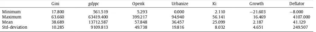
Table 1

The basic statistics.

Gini gdppc Openk Urbanize Ki Growth Deflator

Minimum 17.800 561.519 5.293 0.000 2.110 −21.603 −8.000

Maximum 63.660 63419.400 399.217 94.940 56.141 16.469 4107.000

Mean 38.689 13712.587 57.848 36.457 25.099 2.187 41.129

Std-deviation 10.285 9109.813 49.738 19.816 8.032 4.651 249.507

The semiparametric counterpart of Model (1) with control

1

variables is:

2

giniit

=

g

(

lgdppcit

)

+

x′it

β

+

ui

+

v

it

,

3

t

=

1

,

2

,

· · ·

,

m_i

;

i

=

1

,

2

, . . . ,

n

,

(2)

4

where

v

itis also assumed to be mean-independent ofxit. Since the 5

regressor ‘‘growth’’ may be endogenous (Huang et al., 2009), its

6

lagged form is used in the model.

7

When g

(

·

)

is parametric quadratic, cubic or fourth-degree

8

polynomial functions oflgdppcit,(1) and(2)become parametric 9

unbalanced panel data models with fixed effects. Columns 1–3

10

of Table 2 report the parametric estimation results. Note that

11

a fourth-degree polynomial function is still significant although

12

the coefficient estimates in quadratic and cubic forms are also

13

significant. This casts doubts on the conventional quadratic

14

specification for the relationship.

15

3. Nonparametric estimation and testing method 16

Lety

=

giniandz

=

lgdppc. Models(1)and(2)are estimated by

17

the iterative procedure modified fromHenderson et al.(2008) for

18

unbalanced panel data. Model(1)is used to illustrate the specific

19

modification. To remove the fixed effects, we write

20

˜

yit

≡

yit

−

y1t

=

g

(

zit

)

−

g

(

zi1

)

+

v

it

−

v

i1

≡

g

(

zit

)

−

g

(

zi1

)

+ ˜

v

it

.

21

Denotey

˜

i

=

(

y

˜

i2

, . . . ,

y

˜

imi

)

′_,

_v

_˜

i

=

(

v

˜

i2

, . . . ,

v

˜

imi

)

′_,

∧

gi

=

(

gi2

, . . . ,

22 gimi

)

′_{. The variance–covariance matrix of}

_v

_˜

i and its inverse are 23

calculated asΣi

=

σ

v2

(

Imi−1

+

emi−1emi−1

)

andΣ

−1

i

=

σ

v−2

(

Imi−1

−

24

emi−1emi−1

/

mi

)

, where Imi−1 is an identity matrix of dimension

25

mi

−

1 andemi−1is a

(

mi

−

1

)

×

1 vector of ones. The criterion

26

function is given by

27

Ξi

(

gi

,

gi1

)

= −

1

2

(

y

˜

i

−

gi

+

gi1emi−1

)

′

Σ_i−1

(

y

˜

i

−

gi

+

gi1emi−1

),

28

i

=

1

,

2

, . . . ,

n

.

29

Denote the first derivatives ofΞi

(

gi

,

gi1

)

with respect togit as 30

Ξi,tg

(

gi

,

gi1

)

,t

=

1

,

2

, . . . ,

mi. Then 31

Ξi,1g

(

gi

,

gi1

)

= −

e′mi−1Σ

−1

i

(

y

˜

i

−

gi

+

gi1emi−1

),

32

Ξi,tg

(

gi

,

gi1

)

=

ci′,t−1Σ −1

i

(

y

˜

i

−

gi

+

gi1emi−1

),

t

≥

2

,

33

whereci,t−1is a

(

mi

−

1

)

×

1 matrix with

(

t

−

1

)

th element/other 34

elements being 1

/

0. Denote

(α

0

, α

1

)

′

≡

(

g

(

z

),

dg

(

z

)/

dz

)

′. It can 35

be estimated by solving the first order conditions of the above

36

criterion function iteratively:

37 n



i=1 1 mi mi



t=1

Kh

(

zit

−

z

)

GitΞi,tg 38

×



ˆ

g[l−1]

(

zi1

), . . . ,

Git

(α

0

, α

1

)

′

, . . . ,

g[l−1]

ˆ

(

zimi

)



=

0

,

39

where the argumentΞi,tgisg[l−1]

ˆ

(

zis

)

fors

̸=

t andGit

(α

0

, α

1

)

′ 40

whens

=

t, andg

ˆ

[l−1]

(

zis

)

is the

(

l

−

1

)

th iterative estimates of 41

(α

0

, α

1

)

′. HereGit

≡

(

1

, (

zit

−

z

)/

h

)

′andkh

(v)

=

h−1k

(v/

h

)

,k

(

·

)

42

is the kernel function. The next iterative estimator of

(α

0

, α

1

)

′is 43

equal to



ˆ

g[l]

(

z

),

g

ˆ

[l]

(

z

)



′

=

D−1₁

(

D2

+

D3

)

, where 44

D1

=

n



i=1 1 m_i





e ′ mi−1Σ

−1

i emi−1Kh

(

zi1

−

z

)

Gi1G

′ i1 45

+

mi



t=2

c_i′_,t−1Σ_i−1ci,t−1Kh

(

zit

−

z

)

GitG′it



,

46

D2

=

n



i=1 1 mi





e′_m i−1Σ

−1

i emi−1Kh

(

zi1

−

z

)

Gi1g

ˆ

[l−1]

(

zi1

)

47

+

mi



t=2

c_i′_,t−1Σ_i−1ci,t−1Kh

(

zit

−

z

)

Gitg

ˆ

[l−1]

(

zit

)



,

48

D3

=

n



i=1 1 mi





−

Kh

(

zi1

−

z

)

Gi1e′mi−1Σ

−1

i Hi,[l−1] 49

+

mi



t=2

Kh

(

zit

−

z

)

Gitc′i,t−1Σ −1 i Hi,[l−1]



,

50

andHi,[l−1]is an

(

mi

−

1

)

×

1 vector with elements 51



˜

yit

−

(

g[l−1]

ˆ

(

zit

)

− ˆ

g[l−1]

(

zi1

))



,

t

=

2

, . . . ,

mi

.

52

The series method is used to obtain an initial estimator forg

(

·

)

. The 53

convergence criterion for the iteration is set to be 54

n



i=1 1 mi mi



t=2



ˆ

g[l]

(

zit

)

− ˆ

g[l−1]

(

zit

)



2

/

n



i=1 1 mi mi



t=2

ˆ

g_[l−1]2

(

z_it

) <

0

.

01

.

55

Further, the variance

σ

2

v is estimated by 56

ˆ

σ

_v2

=

1

2n n



i=1 1 m_i

−

1

mi



t=2

(

yit

−

yi1

−

(

g

ˆ

(

zit

)

− ˆ

g

(

zi1

)))

2

.

57

The variance of the iterative estimator g

ˆ

(

z

)

is calculated as 58

κ(

nhΩ

ˆ

(

z

))

−1, where

κ

=



k2

(v)

d

v

, andΩ

ˆ

(

z

)

=

1_n



n i=1

mi−1

mi 59



mi

t=2Kh

(

zit

−

z

)/

σ

ˆ

v2. 60

For the model selection to be data-driven, we modify the 61

specification tests to suit for unbalanced panel data models. We 62

have three specification tests: 63

First, test parametric against nonparametric model in Model(1). 64

The null hypothesisH0is parametric model withg

(

z

)

=

θ

0

(

z

, γ )

. 65

For example,

θ

0

(

z

, γ )

=

γ

0

+

γ

1z

+

γ

2z2. The alternativeH1 66

is thatg

(

z

)

is nonparametric. The statistic for testing this null is 67 I_n(1)

=

1_n



n

i=1 1 mi



mi

t=1

(θ

0

(

zit

,

γ )

ˆ

− ˆ

g

(

zit

))

2, where

γ

ˆ

is a consistent 68

estimator of the parametric model with fixed effects;g

ˆ

(

·

)

is the 69

iterative consistent estimator of Model(1). 70

Second, test parametric against semiparametric model with 71

control variables in Model(2). The nullH0is parametric model with 72 g

(

z

)

=

θ

0

(

z

, γ )

. The alternative is thatg

(

z

)

is nonparametric. The 73

statistic for testing this null isIn(2)

=

1_n



ni=1 1 mi



mi

t=1

(θ

0

(

zit

,

γ )

˜

+

74 x′

it

β

˜

− ˆ

g

(

zit

)

−

xit′

β)

ˆ

2, where

γ

˜

and

β

˜

are consistent estimators in 75

the parametric panel data model with fixed effects;g

ˆ

(

·

)

and

β

ˆ

are 76

[image:6.595.44.566.87.270.2]

X. Zhou, K.-W. Li / Economics Letters xx (xxxx) xxx–xxx 3

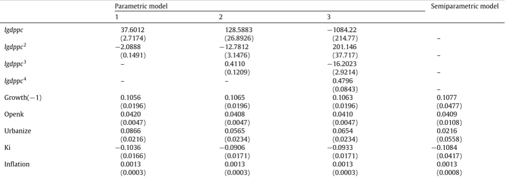
Table 2

Parametric estimation results.

Parametric model Semiparametric model

1 2 3

lgdppc 37.6012 128.5883 −1084.22

(2.7174) (26.8926) (214.77) –

lgdppc2 _{−2.0888 −12.7812 201.146}

(0.1491) (3.1476) (37.717) –

lgdppc3 _{– 0.4110 −16.2023}

(0.1209) (2.9214) –

lgdppc4 _{– – 0.4796}

(0.0843) –

Growth(−1) 0.1056 0.1065 0.1063 0.1077

(0.0196) (0.0196) (0.0196) (0.0477)

Openk 0.0420 0.0408 0.0410 0.0409

(0.0047) (0.0047) (0.0047) (0.0108)

Urbanize 0.0866 0.0565 0.0654 0.0216

(0.0216) (0.0234) (0.0234) (0.0558)

Ki −0.1036 −0.0906 −0.0933 −0.1084

(0.0166) (0.0171) (0.0171) (0.0417)

Inflation 0.0013 0.0013 0.0013 0.0013

(0.0003) (0.0003) (0.0003) (0.0008)

The dependent variable is Gini. The numbers in the parentheses are standard errors of the coefficient estimates. Intercept estimates in parametric models are not reported.

Table 3

Nonparametric estimation ofg(·)at different points of ln(gdppc). Quantile of

z=ln(gdppc)

Nonparametric model(1) Semiparametric model(2)

% z g(z) Std. err. g(z) Std. err. 2.5 7.2014 34.1085 2.9719 32.7535 2.8225 25.0 8.7307 43.3724 1.4581 42.4299 1.3848 50.0 9.4323 38.9278 1.2869 38.7704 1.2222 75.0 9.9073 36.0767 1.0948 35.5236 1.0398 95.0 10.2808 36.1586 1.4052 34.3298 1.3346 97.5 10.3490 36.1649 1.5553 34.0305 1.4771

Third, test the null nonparametric model (1) against the

1

semiparametric model(2). The statistic for testing this null isIn(3)

=

2

1 n



n i=1m1i



mi

t=1

(

g

˜

(

zit

)

− ˆ

g

(

zit

)

−

x′it

β)

ˆ

2_{, whereg}

_˜

₍

_·

₎

_{is the iterative} 3

consistent estimator in Model(1)whileg

ˆ

(

·

)

and

β

ˆ

are the iterative

4

consistent estimator of Model(2).

5

We apply bootstrap procedures to approximate the finite

6

sample null distributions of test statistics and obtain the bootstrap

7

probability values for the three tests.

8

4. Results 9

In the estimation, the kernel is the Gaussian function and the

10

bandwidth is chosen according to rule of thumb. All bootstrap

11

replications are set to be 400. The last column inTable 2reports the

12

coefficient estimation for the control variables in the parametric

13

part of Model (2). Except ‘‘urbanize’’, the coefficient estimates

14

of all other control variables are close to those in parametric

15

models, showing that growth, openness and inflation (investment)

16

significantly increase (reduces) inequality.

17

InTable 3, the nonparametric functiong

(

·

)

is estimated at some

18

quantile points of ln

(

gdppc

)

by using nonparametric Model(1)and

19

semiparametric Model(2). In all these cases, the nonparametric

es-20

timates are slightly larger than their semiparametric counterparts,

21

implying that the overall effect of control variables on inequality is

22

negative. These policy and economic characteristics variables

in-23

deed can affect inequality.

24

Figs. 1and2illustrate the nonparametric estimation ofg

(

·

)

in

25

Models(1)and(2), respectively, where lower and upper bounds

26

of 95% confidence intervals are also drafted. The estimates are

27

acceptable though the estimation has boundary effects. The two

28

curves ofg

(

·

)

in Figs. 1 and 2 look similar, implying that the

29

control variables, though having an overall impact, play little role

30 10 20 30 40 50 60 70

6 7 8 9 10 11

ln(gdppc)

[image:6.595.327.541.289.598.2]

Gini

Fig. 1. g(·)from nonparametric model(1).

10 20 30 40 50 60 70

6 7 8 9 10 11

ln(gdppc)

Gini

Fig. 2. g(·)from semiparametric model(2).

in the estimation of nonlinear shape ofg

(

·

)

.Huang (2004) also 31

reported such findings. The estimation is robust to the control 32

variables. However, the inverted-Uhypothesis is confirmed only 33

when ln

(

gdppc

)

arrives at 7.2, about $1340 of GDP per capita 34

(about 2.5% quantile, seeTable 3). For the case less than this level, 35

inequality decreases with development, though insignificantly, 36

with a very wide confidence interval. This implies that the 37

inverted-Uhypothesis does not significantly hold at low stage of 38

development. 39

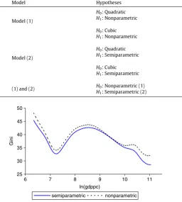
Fig. 3compares the two curves ofg

(

·

)

estimated by nonpara- 40

metric and semiparametric models. The vertical difference be- 41

tween the two curves shows the contribution of control variables 42

4 X. Zhou, K.-W. Li / Economics Letters xx (xxxx) xxx–xxx

Table 4

Model specification tests.

Model Hypotheses Instatistic (p-value) Model selected

Model (1)

H0: Quadratic

9.256 (0.000) Nonparametric

H1: Nonparametric

H0: Cubic _{7.375 (0.003) Nonparametric}

H1: Nonparametric

Model (2)

H0: Quadratic _{11.467 (0.003) Semiparametric}

H1: Semiparametric

H0: Cubic _{11.401 (0.003) Semiparametric}

H1: Semiparametric

(1) and (2) H0: Nonparametric (1) _{5.211 (0.000) Semiparametric}

H1: Semiparametric (2)

25 30 35 40 45 50

6 7 8 9 10 11

ln(gdppc)

Gini

[image:7.595.38.295.91.377.2]

semiparametric nonparametric

Fig. 3. Comparingg(·)from estimating(1)and(2).

variables is positive in reducing inequality. When the development

1

level is below exp

(

9

)

≈

$8100, the net integrated effect has no

sig-2

nificant difference across different development levels. However,

3

when the development level is above exp

(

10

)

≈

$22

,

000, the

con-4

trol variables have a larger integrated effect on inequality, implying

5

that policy instruments and economic performance play a larger

6

role in reducing inequality in the more developed than in less

de-7

veloped economies. For an economy with development between

8

$8100 and $22

,

000, the integrated effect of control variables on

9

inequality is economically insignificant.

10

Table 4presents three kinds of tests in Models(1)and(2). All the

11

nulls are rejected at 1% significant level, showing that parametric

12

form in(1)is inappropriate, but semiparametric specification in

13

(2)is more appropriate for our sample. This justifies our analysis

14

on the estimation of semiparametric model(1).

15

5. Conclusion 16

This paper uses nonparametric and semiparametric unbalanced

17

panel data models with fixed effects to study the validity of

18

the inequality and development relationship. Specification tests

19

justify the flexible semiparametric model. The results show that

20

Kuznet’s inverted-U relationship is confirmed only when the

21

development level arrives at a threshold. The inverted-Udoes not

22

significantly hold when development is less than the threshold.

23

This result is robust whether or not the control variables are

24

included in the model. The integrated contribution of control

25

variables to reduction of inequality is positive. Policy instruments

26

and economic performance play a larger role in reducing inequality

27

in more developed than in less developed economies.

28

Uncited references 29

Q1

Chen, 2003.

30

Acknowledgments 31

Zhou/Li’s research funding was provided by the National 32

Natural Science Foundation of China Grant number 70971143/the 33

City University of Hong Kong Strategic Research Grant number 34

7002433. 35

Appendix. The sample in the study 75 countries and years: 36

Argentina, 1989, 92, 98, 2001. Armenia, 1994–97. Australia, 37

1967–69, 76, 78–79, 81–82, 85–86, 89–90, 94–96, 2002. Austria, 38

1987, 91, 95, 2000. Bahamas, 1970, 73, 75, 77, 79, 86, 88, 91–93. 39

Bangladesh, 1963, 66, 67, 69, 73, 77, 78, 81, 83, 86. Barbados, 1979, 40

96. Belarus, 1995–97, 2002. Belgium, 1979, 85, 88, 92, 96, 2000. 41

Brazil, 1970, 72, 76, 78–91, 93, 96, 98, 2002. Bulgaria, 1981–97, 42

2003. Canada, 1965, 67, 69, 71, 73–75, 77, 79, 81–88, 91, 94, 97, 43

2000. Chile, 1968, 71, 80–94, 98, 2000. China, 1970, 75, 78, 80, 44

82–99, 2001. Colombia 1964, 70, 71, 74, 78, 88, 91, 94, 98, 2003. 45

Costa Rica, 1961, 69, 71, 77, 79, 81, 83, 86, 89, 93, 98, 2001. 46

Cyprus, 1990, 96. Czech Republic, 1991–97, 2002. Denmark, 1963, 47

76, 78–95, 97, 2000. Dominican Republic, 1976, 84, 89, 92, 96, 97, 48

2003. Ecuador, 1968, 88, 93, 94, 95, 98, 2003. El Salvador, 1965, 77, 49

89, 94, 95, 97, 2002. Estonia, 1990–94. Finland, 1962, 77–84, 87, 50

91, 95, 2000. France, 1962, 65, 70, 75, 79, 81, 84, 89, 95. Gabon, 51

1975, 77. Germany, 1973, 75, 78, 80, 81, 83–85, 89, 94, 97, 98, 52

2000. Guatemala, 1986, 87, 89, 98, 2002. Honduras, 1968, 89–94, 53

98, 2003. Hong Kong, 1971, 73, 76, 80, 81, 86, 91, 96, 98. Hungary, 54

1972, 77, 82, 87, 89, 91, 93–97, 99. Ireland, 1973, 80, 87, 94, 99, 55

2000. Israel, 1986, 92, 97. Italy, 1967–69, 71–84, 86, 87, 89, 91, 56

93, 95, 98, 2000. Jamaica, 1958, 2003. Japan, 1962–65, 67–82, 85, 57

88–90, 93, 98, 2002. Kazakhstan, 1993, 96, 2002. South Korea, 1965, 58

66, 70, 71, 76, 80, 82, 85, 88, 93, 98, 2003. Latvia, 1995, 96, 98, 59

2002. Luxembourg, 1985, 91, 94, 98, 2000. Malaysia, 1967, 70, 73, 60

76, 79, 84, 89, 95, 97. Mexico, 1963, 68, 69, 75, 77, 84, 89, 92, 94, 61

98, 2002. Nepal, 1976, 77, 84. Netherlands, 1962, 75, 77, 79, 81–83, 62

1985–99. New Zealand, 1973, 75, 77, 78, 80, 82, 83, 85–87, 89–91. 63

Nicaragua, 1998, 2001. Nigeria, 1959, 81, 82. Norway, 1962, 63, 67, 64

73, 76, 79, 82, 84–91, 95, 96, 2000. Pakistan, 1963, 64, 66, 67, 69, 70. 65

Panama, 1969, 70, 79, 80, 89, 95, 97, 2002. Paraguay, 1990, 95, 98, 66

2001. Peru, 1961, 71, 81, 96, 2002. Philippines, 1961, 65, 71, 75, 85, 67

88, 91, 94, 97. Poland, 1991–97. Portugal, 1973, 80, 89–91, 94, 97. 68

Puerto Rico, 1963, 69, 79, 89. Romania, 1989–92, 94, 98. Russian 69

Federation, 1990, 93–96, 98. Senegal, 1960, 95. Singapore, 1973, 70

78, 80, 89, 92, 97, 2003. Slovak Republic, 1988–97, 2005. Slovenia, 71

1991–93, 97, 2002. South Africa, 1990, 93, 95. Spain, 1965, 73, 75, 72

94, 2000. Sri Lanka, 1963, 69, 73, 79, 80, 81, 86, 87. Sweden, 1963, 73

67, 75, 76, 80–96, 2000. Switzerland, 1982, 92, 2002. Thailand, 74

1962, 68, 69, 71, 75, 81, 86, 88, 90, 92. Trinidad & Tobago, 1971, 75

76, 81, 88, 94. Turkey, 1968, 73, 87, 94, 2003. United Kingdom, 76

1964–76, 79, 85, 86, 91, 95, 2002. United States, 1960–91, 94, 97, 77

2000. Uruguay, 1989, 92, 98. Uzbekistan, 1990, 2002. Venezuela, 78

X. Zhou, K.-W. Li / Economics Letters xx (xxxx) xxx–xxx 5 References

1

Barro, R.J., 2000. Inequality and growth in a panel of countries. Journal of Economic 2

Growth 5, 5–32. 3

Bulí˘r, A., 2001. Income inequality: does inflation matter? IMF Staff Papers 48, 4

139–159. 5

Chen, B.-L., 2003. An inverted-Urelationship between inequality and long-run 6

growth. Economics Letters 78, 205–212. 7

Henderson, D.J., Carroll, R.J., Li, Q., 2008. Nonparametric estimation and testing of 8

fixed effects panel data models. Journal of Econometrics 144, 257–275. 9

Huang, H.-C.R., 2004. A flexible nonlinear inference to the Kuznets hypothesis. 10

Economics Letters 84, 289–296. 11

Huang, H.-C.R., Lin, Y.-C., Yeh, C.-C., 2009. Joint determinations of inequality and 12

growth. Economics Letters 103, 163–166. 13

Iradian, G., 2005 Inequality, poverty, and growth: cross-country evidence. IMF 14

Working Paper No. 05/28. 15

Li, H., Squire, L., Zou, H.-F., 1998. Explaining international and intertemporal 16 variations in income inequality. Economic Journal 108, 26–43. 17 Lin, S.-C., Huang, H.-C., Weng, H.-W., 2006. A semiparametric partially linear 18 investigation of the Kuznets’ hypothesis. Journal of Comparative Economics 34, 19

634–647. 20

Milanovic, B., 2005. Worlds Apart: Measuring International and Global Inequality. 21

Princeton University Press. 22