www.hydrol-earth-syst-sci.net/16/1623/2012/ doi:10.5194/hess-16-1623-2012
© Author(s) 2012. CC Attribution 3.0 License.
Earth System
Sciences
Satellite remote sensing of water turbidity in Alqueva reservoir and
implications on lake modelling
M. Potes1, M. J. Costa1,2, and R. Salgado1,2
1Evora Geophysics Centre (CGE), University of ´´ Evora, Rua Rom˜ao Ramalho 59, 7000-671 ´Evora, Portugal
2Department of Physics, University of ´Evora, Rua Rom˜ao Ramalho 59, 7000-671 ´Evora, Portugal
Correspondence to: M. Potes ([email protected])
Received: 7 October 2011 – Published in Hydrol. Earth Syst. Sci. Discuss.: 21 December 2011 Revised: 23 April 2012 – Accepted: 11 May 2012 – Published: 6 June 2012
Abstract. The quality control and monitoring of surface freshwaters is crucial, since some of these water masses con-stitute essential renewable water resources for a variety of purposes. In addition, changes in the surface water compo-sition may affect the physical properties of lake water, such as temperature, which in turn may impact the interactions of the water surface with the lower atmosphere.
The use of satellite remote sensing to estimate the water turbidity of Alqueva reservoir, located in the south of Por-tugal, is explored. A validation study of the satellite derived water leaving spectral reflectance is firstly presented, using data taken during three field campaigns carried out during 2010 and early 2011. Secondly, an empirical algorithm to es-timate lake water surface turbidity from the combination of in situ and satellite measurements is proposed. Finally, the importance of water turbidity on the surface energy balance is tested in the form of a study of the sensitivity of a lake model to the extinction coefficient of water (estimated from turbidity), showing that this is an important parameter that affects the lake surface temperature.
1 Introduction
Water quality of reservoirs is determined by physical and chemical properties. Thus, the success of reservoir man-agement depends on the detection of spatial and temporal changes in the reservoir status that reflect natural and anthro-pogenic alterations in the surrounding environment (Chap-man, 1996; Lee and Walter, 1997; Morais et al., 2007). Lakes strongly affect the structure of the atmospheric bound-ary layer (see, for example, Zilitinkevich et al., 1991) and
therefore the weather and the climate on a variety of scales. However, until very recently, the numerical weather predic-tion (NWP) models did not include an explicit representa-tion of the evolurepresenta-tion of lake properties. Currently, many ef-forts are being made to include 1-D lake parameterization schemes in operational numerical weather prediction (NWP) models (e.g. Mironov et al., 2010; Salgado and Le Moigne, 2010; Dutra et al., 2010). The two layer bulk lake model, FLake (Mironov, 2008), enjoys growing popularity in NWP and climate models as well as in limnology. Examples of the impact of the inclusion of these schemes on weather forecast and climate models can be found in Balsamo et al. (2012) and Kheyrollah Pour et al. (2012) and references therein. The FLake model includes the following optical parameters: sur-face albedo, long wave emissivity and light extinction coeffi-cient. The water extinction coefficient only rarely is directly measured. On the contrary, there are some studies aiming at relating turbidity measurements with extinction coefficients (Parkhill and Gulliver, 2002; Giblin et al., 2010); neverthe-less, these relationships depend on the water mass conditions (combination of organic and inorganic material present in the water mass).
Turbidity is an optical property of the water body – a mea-sure of the amount of light scattered and absorbed by parti-cles in the water column (Michaud, 1991). Turbidity may in-duce changes in the lake’s vertical thermal structure, which in turn plays an important role in autochthonous primary pro-duction (Friedl and W¨uest, 2002) and in the evolution of the water surface temperature, which is a key variable in the water-atmosphere transfers.
programs. However, samples regularly collected and anal-ysed in the laboratory are spatially and temporally limited. Thus, the use of satellite data to evaluate the optical wa-ter properties is steadily increasing, since this kind of data provides undoubtedly the only way to proceed for global characterization of reservoirs (Koponen et al., 2002; Chen et al., 2006; Tyler et al., 2006; Simis et al., 2007; Alikas and Reinart, 2008; Duan et al., 2008; Gitelson et al., 2008; Gons et al., 2008).
According to Moore (1980), the feasibility of measuring water color and turbidity from satellites can be assessed by considering light and water interaction processes and by eval-uating the effects of atmospheric and hydrological variables. Note that the many Low Earth Orbit satellite instruments launched in the last decade constitute exceptionally valu-able tools for quantitative analysis of surface water qual-ity (Gordon and Wang, 1994; Dickey et al., 2006). Their multi-spectral and spatial resolution capabilities allow for improved techniques in retrieving the optical properties of lake water. A good example is the MEdium Resolution Imag-ing Spectrometer (MERIS) onboard ENVIronmental SATel-lite (ENVISAT), which combines moderately high spatial resolution (260 m×290 m at nadir) with an adequate spec-tral resolution in the visible and near infra-red regions (ESA, 2008). Higher spatial resolution satellite systems are avail-able, but there are difficulties associated with their use: on one hand their long revisit cycle and on the other hand the related expenses. The use of MERIS represents a good com-promise in order to have a low-cost, frequent (nominal revisit time of 2–3 days at midlatitudes) monitoring of inland water bodies. The potential of using satellite remote sensing data to obtain information on lake water turbidity is demonstrated in this work.
Potes et al. (2011) recently developed a method to retrieve surface freshwater biological parameter (chlorophylla and cyanobacteria) concentrations over Alqueva reservoir (south of Portugal) from MERIS satellite data, aiming at providing full spatial coverage and continuous monitoring of these pa-rameters that affect the water quality. The methodology is now adapted and presented here to obtain a new empirical algorithm allowing for the retrieval of the water turbidity of the same reservoir, which is important for the estimation of water extinction coefficients.
The present work has three main goals: firstly, the vali-dation of the atmospheric correction methodology; secondly, the development of a satellite-based remote sensing method to retrieve surface inland freshwater turbidity, which is a measure of water quality characterizing optical behavior and deemed an essential parameter towards the improvement of lake parameterization schemes in weather forecast and cli-mate models; and thirdly, as a natural consequence of the previous aim, it is an objective of this work to show the im-portance of the lake optical characteristics in the evolution of lake surface temperature and heat fluxes. This is done through a sensitive analysis of the FLake model results to
different values of the water extinction coefficient, represent-ing here possible extreme water turbidity cases.
The following section gives a description of the data and methods used. Sects. 3 and 4 present the results and Sect. 5 summarizes the conclusions.
2 Study site, data and methods
The Alqueva reservoir, located in the south of Portugal along 83 km of the main course of the Guadiana River, constitutes the largest artificial lake in the Iberian Peninsula (Fig. 1). At the full storage level of 152 m, the reservoir has a total ca-pacity of 4.150 km3and a surface area of 250 km2. Filling of Alqueva reservoir began in February 2002 and lasted about one year to reach a stable storage level of about 135 m.
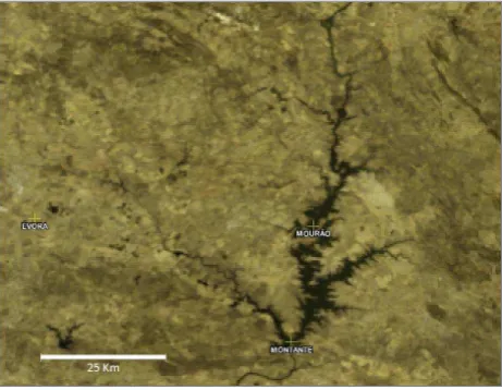
According to Morais et al. (2007), Alqueva reservoir was classified as eutrophic based on total phosphorus (>35 mg P m−3) and chlorophylla (<10 µg l−1) concentra-tions. The Alqueva water quality control belongs to a large monitoring programme implemented by the Portuguese com-pany responsible for Alqueva exploitation (Empresa de De-senvolvimento e Infra-Estruturas de Alqueva, EDIA). The monitoring programme was implemented at the beginning of the filling phase. Nevertheless, this control is spatially and temporally limited. Monthly water samples are collected in a few spots of the reservoir, and afterwards analyzed in labo-ratory. Two sites were selected (up to 500 m from the shore) for the validation presented in this study, taking into account not only their geographical positions inside the reservoir, but also the corresponding satellite image pixel dimensions (260×290 m) that should enclose a homogeneous surface. Figure 1 illustrates the location of these sites, namely Mour˜ao and Montante. The selection of these sites aims, in addition, to reduce as much as possible the adjacency effects, consist-ing of the brightenconsist-ing of dark water pixels due to reflections from neighboring land (vegetation or soil) pixels with higher reflectances, which reach the sensor and appear to come from a water pixel, thereby reducing the contrast between water and land pixels.
In March 2002 the European Space Agency (ESA) launched ENVISAT (ENVIronmental SATellite), an ad-vanced polar-orbiting Earth observation satellite which pro-vides complete coverage of the globe within one to three days (ESA, 2008).
The MEdium Resolution Imaging Spectrometer (MERIS), onboard ENVISAT, measures the solar reflected radiation from the Earth, ranging from the visible to the near infrared (400 to 1040 nm). These spectral bands were carefully cho-sen in accordance with the mission goals and priorities of the MERIS instrument, to ensure practical applicability of the sensor.
27 Figure 1. MERIS image showing Alqueva reservoir location and position of the sites used in the
study. The city of Évora is also indicated as a point of reference.
Fig. 1. MERIS image showing Alqueva reservoir location and posi-tion of the sites used in the study. The city of ´Evora is also indicated as a point of reference.
maximum spatial resolution of 260×290 m at the nadir. The selection of the MERIS images was based on three condi-tions: (i) minimum time lag between MERIS and limnolog-ical sampling dates, due to possible alterations of the wa-ter surface paramewa-ters (one day difference); (ii) cloud-free conditions (MERIS cloud mask); and (iii) lack of aerosol events (generally desert dust or forest fire smoke). A wa-ter mask is applied to identify inland wawa-ters pixels from Alqueva reservoir. The test relies on the TOA (top of the atmosphere) spectral reflectances, with the conditions that band 6 (620 nm)>band 10 (753.75 nm) and band 13 (865 nm)<0.1.
2.1 Atmospheric correction validation
The assessment of the retrieval reliability is highly depen-dent on the comparison with independepen-dent measurements that allow for error estimation and eventually achieve a vali-dation of the method (Dickey et al., 2006). The study of surface water properties from satellite remote sensing tech-niques requires the correction of atmospheric effects. The present study is applied only to cloud-free days over Alqueva reservoir. Major gas absorption bands are avoided as well; therefore, the atmospheric correction depends essentially on the type and amount of aerosols present in the atmo-sphere. Aerosol event situations are also discarded, and thus only clean background aerosol conditions are being con-sidered (Elias et al., 2006). A comprehensive description of the atmospheric correction methodology used is given by Potes et al. (2011). The aerosol measurements (optical thickness, size distribution, and complex refractive index) continuously taken at the observatory of the ´Evora Geo-physics Centre (CGE), as part of the AErosol RObotic NET-work (AERONET) (Holben et al., 2001), are used in the
atmospheric correction. This is done assuming that there is not a significant variation in the aerosol conditions between
´
Evora and the Alqueva area (horizontal distance of about 50 km); most of the time this is an accurate approximation, except in the case of aerosol events (Elias et al., 2006). The radiative transfer code adopted for the atmospheric correc-tion was the Second Simulacorrec-tion of the Satellite Signal in the Solar Spectrum (6S) developed by Vermote et al. (1997). The 6S can simulate satellite radiation measurements in cloud-free atmospheres between 0.25 and 4.0 µm, for a wide range of atmospheric and surface conditions, taking into account the main atmospheric compounds and considering 34 atmo-spheric levels distributed from the ground up to 100 km alti-tude. The adjacency effects due to reflection from contiguous pixels are also taken into account in the algorithm (consider-ing water, and vegetation or soil surface) accord(consider-ing to the neighbouring pixel classifications (Potes et al., 2011).
During 2010 and 2011 three field campaigns were carried out in Alqueva reservoir to measure the water leaving spec-tral reflectance, with the aim of validating the satellite atmo-spherically corrected spectral reflectance. A portable spectro-radiometer (FieldSpec UV/VNIR) from ASD Inc. was used for this purpose, and the water leaving spectral reflectance was measured across the spectral range 325–1075 nm with 1 to 3 nm spectral resolution from visible to near infrared. The campaigns took place at Mour˜ao site on 27 July 2010, Mour˜ao and Montante sites on 25 August 2010 and at three distinct places near Mour˜ao site on 24 February 2011.
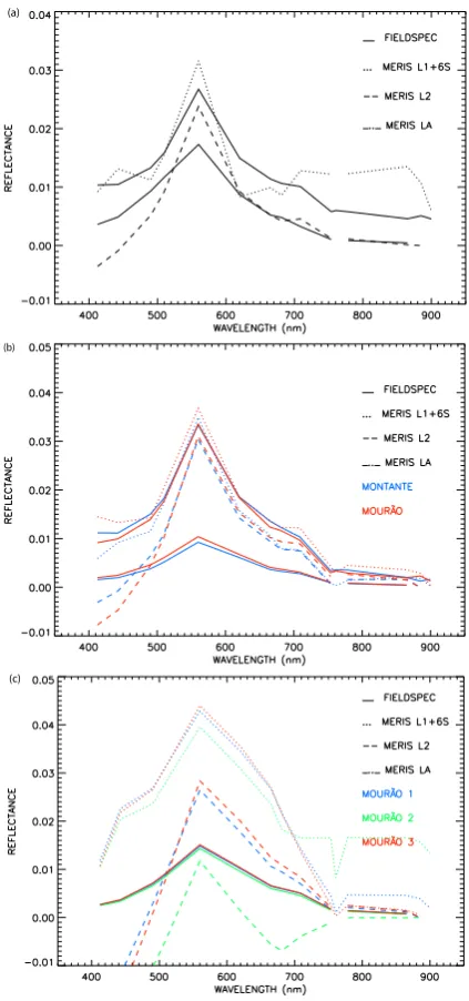
Figure 2 shows a comparison between the measured and satellite-derived water leaving reflectance, obtained for the three field campaigns carried out. The measured spectrum is identified as FieldSpec (solid line) and it corresponds to the average of ten measured spectra. The different satellite-derived spectra correspond to the: (i) atmospheric correction developed by the authors (Potes et al., 2011), hereinafter re-ferred to as MERIS L1+6S; (ii) MERIS level 1b lake algo-rithm (Doerffer and Schiller, 2008), referred to as MERIS LA; and (iii) MERIS level 2, identified as MERIS L2. Note that the atmospheric correction scheme developed by the au-thors (MERIS L1+6S) is the one that better matches the mea-sured water leaving reflectance for the three campaigns car-ried out. In Fig. 2c the MERIS L1+6S spectrum for Mour˜ao 2 presents high values of reflectance in the near-infrared spec-tral region, which can be attributed to the lesser distance from shore with respect to Mour˜ao 1 and 3, resulting in the con-tamination of the MERIS pixel by vegetation present in the nearby land pixels in this period of the year.
Table 1 presents the statistical parameters of the regres-sions obtained for each of the campaigns, considering the MERIS L1+6S retrieval and the field measurements. The data points for each campaign correspond to the number of spectral bands available from the MERIS images for each of the sites where measurements are taken.
[image:3.595.52.283.65.244.2]Table 1. Parameters obtained in the correlation between the measured and satellite-derived water leaving spectral reflectance (MERIS L1+6S) for the three field campaigns carried out. The parameters are the following: number of data (N), equation of the regression, correlation coefficients (R), root mean squared errors (RMSE) and normalized root mean squared errors (NRMSE).
Campaign date N Regression equation R RMSE NRMSE (%)
27 July 2010 14 0.73x+ 0.012 0.64 0.01 46 25 August 2010 30 1.04x−0.0007 0.96 0.002 8 24 February 2011 45 0.77x+ 0.008 0.87 0.007 16
Table 2. Parameters obtained in the correlation between the measured and satellite-derived water leaving spectral reflectance for the three methods that are compared. The parameters are the same as in Table 1.
Method N Regression equation R RMSE NRMSE (%)
MERIS L1+6S 89 0.86x+ 0.0050 0.84 0.007 14 MERIS L2 78 0.28x−0.0003 0.27 0.020 33 MERIS LA 72 −0.08x+ 0.0060 −0.21 0.012 27
with a correlation coefficient of 0.96 and a normalized root mean squared error of 8 %. A slightly worse agreement was found for 27 July 2010, with a correlation coefficient of 0.64 and a normalized root mean squared error of 46 %; nonethe-less, the linear correlation was still significant for a 95 % con-fidence interval. In fact, on 27 July 2010 a minor desert dust transport event was starting to affect the area with aerosol op-tical depths (at 440 nm) that reached 0.26, whereas for clean background situations the aerosol optical depth at 440 nm is lower than 0.12 (Elias et al., 2006). In these cases the at-mospheric conditions can hardly be considered spatially ho-mogeneous, therefore the situation between ´Evora (where the aerosol measurements are taken) and Alqueva may be somewhat different and the atmospheric correction results reflect this. On 24 February 2011, MERIS FR image data was not available due to issues connected with ESA acquisi-tion strategy; therefore the satellite image used in this cam-paign is the MERIS reduced resolution (1200 m at nadir). The major problems arising in this case are mainly con-nected to pixel dimension, and since Alqueva is not a very large lake, the difficulties associated with adjacency effects increase. Nevertheless, a correlation coefficient of 0.87 and a normalized root mean squared error of 16 % were found. In summary, measurements were taken at six sites during the three field campaigns: Mour˜ao site on 27 July 2010, Mour˜ao and Montante sites on 25 August 2010 and three dis-tinct places near Mour˜ao site on 24 February 2011. MERIS L1+6S has 15 spectral bands which would supply a total of 90 points; nevertheless, atmospheric correction failed for one of the data points (the reflectance was negative) and there-fore 89 data points were available. MERIS L2 is provided with 13 spectral bands which give a total of 78 data points. MERIS algorithm from Doerffer and Schiller (2008) is pro-vided with 12 spectral bands summing 72 points. Table 2 summarizes the statistical parameters of the regressions ob-tained for each of the three atmospheric correction methods
considered. It should be noted that the atmospheric correc-tion applied according to the methodology proposed by Potes et al. (2011) (MERIS L1+6S) presents the best fit with Field-Spec measurements, with a correlation coefficient of 0.84, whereas both MERIS L2 and LA present pretty low corre-lation coefficients of 0.27 and−0.21, respectively. Also the NRMSE values for the latter two methods (33 % and 27 %) are about twice the value obtained for MERIS L1+6S, which is 14 %. Since the empirical algorithm presented in next sec-tion is band-specific (i.e., uses bands centred at 412.5 nm and 560 nm), the correlation coefficients and NRMSE are also calculated using only these two spectral bands. MERIS L1+6S presents once again the highest correlation coeffi-cient with a value of 0.93 and a NRMSE of 16 %, whereas MERIS L2 and LA present correlation coefficients of 0.79 and 0.87 and NRMSE of 65 and 49 %, respectively. These results hint at the need for a specific atmospheric correction in the Alqueva area, allowing the use of water leaving spec-tral reflectances to accurately estimate water quality related parameters.
2.2 Empirical algorithm
The water leaving spectral reflectance obtained through at-mospheric correction of TOA satellite data is related with in situ measurements of water turbidity, resulting in an algo-rithm which allows for the estimation of the water turbid-ity based upon the ratio of spectral reflectances (Bukata et al., 1995; Sathyendranath, 2000). This kind of technique was proposed before by Koponen et al. (2002) to monitor water turbidity in Finnish Lakes, and Chen et al. (2006) has applied a similar methodology in Tampa Bay (Florida, USA).
(a)
(b)
[image:5.595.61.273.61.513.2](c)
Fig. 2. Comparison between the measured and satellite-derived wa-ter leaving reflectance spectra for the three field campaigns: (a) 27 July 2010, (b) 25 August 2010 and (c) 24 February 2011. The measured spectra are identified as FieldSpec (solid line) and the satellite-derived are MERIS L1+6S (dotted), MERIS L2 (dashed) and MERIS LA (dash dot dot).
combinations and selecting the one with the highest cor-relation coefficient. The algorithms proposed by H¨arm¨a et al. (2001), Koponen et al. (2002) and Chen et al. (2006) found in the red and near infrared spectral bands the best fits, and consequently the empirical algorithms to retrieve water turbidity. Yet, in this study, the best fit found uses a ratio be-tween green and blue spectral regions. The sensitivity to dif-ferent spectral regions may be explained by the characteris-tics of the turbidimeter employed to measure water turbidity
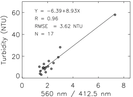
in Alqueva, which uses a tungsten lamp operating between 400 and 600 nm, the same spectral range found to be the best combination for the empirical algorithm. The best fit between in situ water turbidity and atmospherically corrected satel-lite spectral reflectance combinations was revealed to be of linear type using the ratio between the green (560 nm) and blue (412.5 nm) MERIS spectral bands, with a rather high correlation coefficient of 0.96 (Fig. 3). A total number of 17 data points are used, corresponding to the two locations considered (Fig. 1) and to the period of study, taking into ac-count the conditions imposed for the MERIS image selection (cloud-free sky, lack of aerosol events and minimum time lag between MERIS and limnology dates).
Note that the highest turbidity point of almost 60 NTU (Fig. 3), recorded at Mour˜ao site, plays an important role in the linear correlation found (0.96); nevertheless, if the referred point is removed from the dataset, the linear cor-relation is still significant for a 99 % confidence interval (R= 0.82). The empirical algorithm obtained is then used to estimate the water turbidity over the whole Alqueva reservoir surface area, as exemplified in Sect. 3.
In general, light intensity declines exponentially with depth, as described by the Beer-Lambert Law:
Iz=I0e−kz (1)
whereIzis the light intensity at a depthzbelow the surface,
I0is the immediate sub-surface light intensity,zis the depth
interval betweenI0andIz, andkis the rate of attenuation of
downwelling radiation, usually referred to as the extinction coefficient.
Fig. 3. Scatter plot between water turbidity (NTU) and the ratio be-tween MERIS band 5 (560 nm) and band 1 (412.5 nm). Also shown the linear regression obtained.
2.3 FLake model
The FLake model, fully documented in Mironov (2008), is intended for use as a lake parameterization scheme in merical weather prediction, climate modelling, and other nu-merical prediction systems for environmental applications. It is based on a two-layer representation of the evolving tem-perature profile and on the integral energy budgets for the two layers. The structure of the stratified layer between the upper mixed layer and the basin bottom, the lake thermo-cline, is described using the concept of self-similarity of the temperature-depth curve. This concept, based on empirical evidence with some theoretical support, assumes that the di-mensionless temperature8profile in the thermocline can be fairly accurately parameterized through a universal function of dimensionless depth:
8 (ζ )=TS−T (z)
TS−TBOT
;ζ= z−h
D−h (2)
where z is the depth, TS is the mixed-layer surface
tem-perature,TBOT is the temperature at the lake bottom, h is
the thickness of the mixed-layer, and D is the total lake depth. (D − h) is the thermocline depth. Several polyno-mial approximations for 8 may be found in the literature (see Mironov, 2008). In FLake, a 4th order polynomial is assumed for8, and its shape is completely defined by its integral betweenζ= 0 andζ= 1, which is the shape factor,
CT. The dimensionless shape factor varies between a
min-imum value, 0.5, corresponding to a mixed layer stationary state or retreat, and a maximum value, 0.8, the maximum al-lowed curvature in the mixed layer deepening process. With this assumption, the water temperature profile is completely described by the four variables:TS,TBOT,handCT; and one
fixed parameter:D.
01-0 1-20
09
15-0 1-20
09
29-0 1-20
09
12-0 2-20
09
26-0 2-20
09
12-0 3-20
09
26-0 3-20
09
m
m
[image:6.595.315.544.63.247.2]0 5 10 15 20 25 30 35
Fig. 4. Daily precipitation recorded in ´Evora Geophysics Centre, from January to March 2009.
In order to solve the energy balance equations for the two layers, the short-wave radiative flux is computed using the exponential approximation of the decay law (Eq. 1). The light extinction coefficient in water (kin Eq. 1), similar to other optical characteristics of water, is lake-specific and time de-pendent, and should hence be estimated with caution in every particular case. Up to 8 spectral bands characterized by dif-ferent extinction coefficients may be considered in FLake.
The FLake model also includes optional schemes for the representation of upper layers of ice and snow and a bottom layer of sediments. The first ones were not activated in the present work as lake waters do not freeze in the region. The evolution of the vertical temperature structure of the ther-mally active layer of bottom sediments is computed using the same concept of self-similarity.
3 Case study results
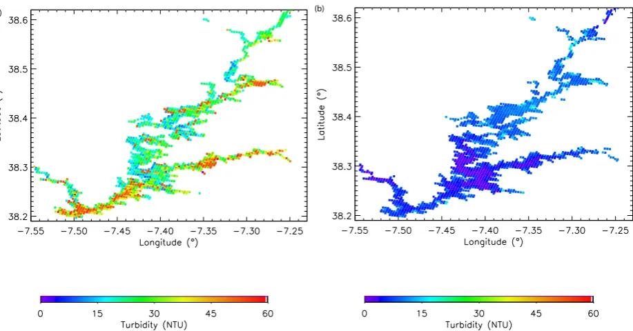
A nearly continuous precipitation event that occurred dur-ing January and the first week of February 2009 (Fig. 4), in the south of Portugal, with roughly 210 mm of accumulated precipitation in 41 days, was recorded at ´Evora–Verney Me-teorological station ( ´Evora Geophysics Centre). Strong and continuous precipitation in the area causes a run-off, mainly by the Guadiana River, which usually introduces organic and inorganic matter into Alqueva reservoir, leading to an in-crease of water turbidity.
(a) (b)
Fig. 5. Turbidity maps for Alqueva reservoir on (a) 11 February 2009 and (b) 15 March 2009.
15 March 2009 (1 month after the precipitation event), where the lake presents rather low turbidity values (<10 NTU).
These results constitute a strong indication that the em-pirical algorithm derived provides meaningful turbidity val-ues. Further turbidity measurements, which are not available presently, will extend the turbidity limits, strengthen the cor-relation and validate the empirical algorithm.
4 FLake sensitivity to the extinction coefficient of sunlight
In order to investigate the importance of turbidity in the evo-lution of the lake surface water temperature, a sensitivity test of the FLake model to the water extinction coefficient was conducted.
The test consisted of FLake stand-alone simulations forced by atmospheric data collected at the Alqueva reservoir, using typical minimum and maximum expected extinction coeffi-cients of 1.0 m−1(clear water) and 6.1 m−1(turbid water).
The model runs were carried out for May and June 2007 (61 days). In this period, the water column was thermally stratified. The forcing consists of time series of the hourly averaged meteorological variables – pressure, air moisture and temperature, wind speed, and solar global radiation – collected at the Mour˜ao meteorological station. This sta-tion belongs to the Portuguese Water Institute (INAG) and is installed on a floating platform located near the Mour˜ao site (see Salgado and Le Moigne, 2010, for a description of this type of station). The data are available at the site http://snirh.pt. Since the downward longwave radiation flux
is not measured at the station, though it is also needed, it was obtained from linear interpolation of the 3-hourly output of the ECMWF IFS weather forecast model.
The initial conditions were constructed from hourly wa-ter temperature observations collected at the same point. Un-fortunately, the water temperature measurements are only available at 3 levels (surface, middle and bottom), which are not sufficient to adjust a FLake initial profile characterized by four variables. Thus, only the initial bottom temperature and the surface mixed layer temperature were taken directly from the observations. The other initial values (CT andh)
were obtained by tuning (calibrating) the model to repro-duce the measured water surface temperature dataset. Due to the complex topographical characteristics of the artificial reservoir, the lake depth,D, which is not a local but an ef-fective or spatially-averaged parameter, was also estimated by the tuning workout. In the tuning simulations, the value of the extinction coefficient corresponding to turbid water (k= 6.1 m−1)was imposed. In the tuning process, 3 parame-ters were considered free (fixed depth,D, and initial values for handCT). The model ran for an ensemble of realistic
values for these variables:D between 10 and 50 m, with a step of 1 m; hbetween 1 and 20 m, step 1 m; CT between
0.50 and 0.80 (all range), step 0.01. This means that about 24 000 simulations were performed for the 61 day period. The configuration which minimized the root mean square error between modelled and observed hourly mean surface temperature was chosen. After this procedure, the follow-ing parameters and initial conditions were used: D= 23 m,
(a)
0 6 12 18 0
06/06/2007 Hour 21
22 23 24 25 26
Te
m
p
er
at
u
re
(C
)
MODEL OBSERVATIONS Water Temperature
Extinction coefficient: 1.0 m-1
0 6 12 18 0
06/06/2007 Hour
21 22 23 24 25 26
Te
m
p
er
at
u
re
(C
)
MODEL OBSERVATIONS
Water Temperature
Extinction coefficient: 6.1 m-1
(b)
0 10 20 30 40 50 60
Day after 01/05/2007 15
20 25 30
Te
m
p
er
at
u
re
(C
)
MODEL OBSERVATIONS Water Temperature
Extinction coefficient: 1.0 m-1
(c)
0 10 20 30 40 50 60
Day after 01/05/2007 15
20 25 30
Te
m
p
er
at
u
re
(C
)
MODEL OBSERVATIONS Water Temperature
Extinction coefficient: 6.1 m-1
Extinction coefficient: 6.1 m-1
Extinction coefficient: 6.1 m-1
[image:8.595.70.526.68.402.2](d)
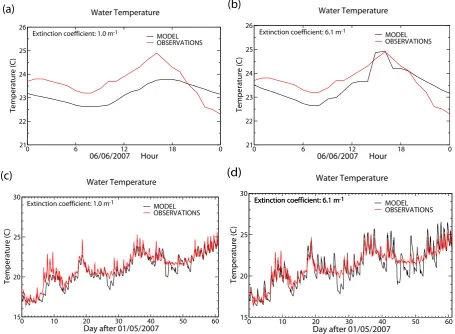
Fig. 6. Comparison between the lake water surface temperature observed and modeled with FLake for: (a) 6 June 2007 with an extinction coefficient of 1.0 m−1 (simulation Mo10); (b) 6 June 2007 with an extinction coefficient of 6.1 m−1 (simulation Mo61); (c) May and June 2007 with an extinction coefficient of 1.0 m−1(simulation Mo10); (d) May and June 2007 with an extinction coefficient of 6.1 m−1 (simulation Mo61).
Each simulation was performed for 61 days using a time step of 30 min. The initial conditions, the lake depth and the forcing were the same for all the simulations, which only differ on the extinction coefficient. Only the two ex-treme cases, corresponding to turbid and clear water values, ofk= 6.1 m−1(simulation Mo61) andk= 1.0 m−1 (simula-tion Mo10), will be analyzed and discussed. In the following, the simulations will be identified respectively by Mo61 and Mo10.
As expected and shown in Fig. 6a and b, the simula-tion Mo61 better reproduces the water surface diurnal cy-cle on 6 June (the day when the highest turbidity value was recorded); in particular, the modeled daily amplitude (around 2◦C) is close to the observed one and higher than that obtained in the Mo10 (around 1◦C). In the late after-noon and evening, the observed water surface temperature dropped sharply due to the occurrence of strong wind, a fea-ture not fully represented by the model, even in the Mo61 simulation.
The lower the coefficient of the extinction, the lower the daily temperature range is. This is visible on this particular day, and also during the entire period, as shown in Fig. 6c and d. The respective figures shows that surface temperature variations are more sudden in the Mo61 simulation. This is not an unexpected result, since when the water is more turbid, solar radiation will penetrate less deeply and therefore will be more absorbed in the surface layer, thereby heating it.
The results show that there are periods when the observed evolution is better reproduced by the simulation Mo61 (the first 10 days, for example), while, by contrast, others are bet-ter represented in the Mo10, corresponding to days with less thermal amplitude (days 45 to 55, for example). It is possi-ble that the periods best represented by the Mo61 simulation correspond to days of higher water turbidity and vice versa. Unfortunately, we lack a turbidity time series in order to con-firm this assumption.
important differences in the lake surface temperature, which is a relevant parameter for heat and moisture transfers be-tween water bodies and the atmosphere. Under the conditions assumed in the present sensitivity test, the daily mean sur-face temperature range jumps from about 1.2◦C in the Mo10 (with a maximum of about 2.8◦C) to 2.4◦C in the Mo61 (with a maximum of about 5.3◦C).
In both cases, but more clearly in the Mo61, the simu-lated surface (mixed layer) water temperatures show some events of sudden daily change not visible in the measured one. These events are initiated with a sharp fall in the sur-face layer temperature due, in the simulations, to the rapid increase of the mixed layer depth,h, which passes (in Mo61) from values less than 2 m to values greater than 8 m (not shown). Thus, the decrease in simulated temperature is due to the fact that the mixture brings deeper (colder) water to the surface. In turn,hincreases due to the occurrence of high speed wind events (greater than 10 m s−1).
In reality, this fact was not observed in the studied period. The difference between model and observations may be due to errors in wind measurements or, more likely, to horizon-tal mixtures not expected to be represented in 1-D models, which bring water from areas where the lake depth is lower thanh and therefore do not cool. Another explanation may be an incorrect representation of the evolution ofhin windy conditions when the lake water is very stratified. This possi-bility needs further investigation.
These differences in surface temperature have effects in the patterns of surface sensible heat flux,H, and evaporation,
E. For the whole simulation period, the increase in simulated sensible heat flux between Mo10 and Mo61 is about 7 %. The simulated difference in total evaporation is relatively smaller, with the evaporation being about 3 % higher for the simula-tion with higher turbidity (Mo61). The results thus indicate that more turbid lake waters tend, during the heating season, to prevent heating of the whole water column (leading to less heat storage) and transfer the energy faster to the atmosphere, resulting in a colder lake. In the end of the simulation period, the column mean water temperature is 0.3◦C higher in Mo10 than in Mo61.
5 Conclusions
A satellite based methodology was developed and applied to retrieve the surface water turbidity of Alqueva reservoir in the south of Portugal. An important aspect of the satellite data used for surface applications is the atmospheric correc-tion process. A validacorrec-tion of the atmospheric correccorrec-tion is presented based on the comparison between ground based and atmospherically corrected spectral reflectance measure-ments obtained during three field campaigns carried out in Alqueva throughout 2010 and early 2011. A correlation co-efficient of 0.84 and a NRMSE of 14 % were obtained for the comparison, which were deemed adequate, especially when
compared to different atmospheric correction algorithms that are probably not suited for the Alqueva lake area.
The empirical algorithm proposed to estimate surface wa-ter turbidity from atmospherically corrected satellite spectral reflectance is of linear type and combines green (560 nm) and blue (412.5 nm) spectral regions, presenting a high cor-relation coefficient of 0.96. Since only 17 data points were available for the study, new field campaigns are planned for Alqueva reservoir including turbidity as well as spectral re-flectance and light extinction measurements. This is aimed at strengthening the confidence on the turbidity algorithm proposed, extending the turbidity limits and deriving a proper relation for the Alqueva lake extinction coefficient. Neverthe-less, the turbidity spatial distribution obtained for the whole lake, for a case study, provided meaningful results.
A sensitivity study of the FLake model to the water extinc-tion coefficient was also conducted in order to investigate the importance of turbidity in the evolution of the lake surface water temperature. Results show that the model is very sen-sitive to different extinction coefficient values and that vari-ations in turbidity can lead to significant changes in the lake surface temperature, which is a parameter that plays a central role in heat and moisture transfers between the lake and the atmosphere. The results also indicate that the turbidity of wa-ter should be taken into account in lake schemes inside high-resolution weather forecast models. While it is not possible to include this parameter in assimilation systems, we sug-gest the setup of time-dependent global climatological maps of the light extinction coefficient of lake waters be used by the forecast models. Those maps may be built following the satellite based methodology described in this work.
Acknowledgements. This work is financed through FEDER
(Pro-grama Operacional Factores de Competitividade – COMPETE) and National funding through FCT – Fundac¸˜ao para a Ciˆencia e a Tecnologia in the framework of projects 01-0124-FEDER-007122 (PTDC/CTE-ATM/65307/2006) and FCOMP-01-0124-FEDER-009303 (PTDC/CTE-ATM/102142/2008) and through FCT grant SFRH/BD/45577/2008. Image data has been provided by ESA in the frame of ENVISAT projects AOPT-2423 and AOPT-2357. We thank AERONET investigators for their effort in establishing and maintaining ´Evora AERONET site. We also thank the Water Laboratory of the University of ´Evora for support in the field campaigns and EDIA for providing the water quality data used in this work. We are grateful to the Portuguese Institute of Meteorology and ECMWF for MARS database account.
References
Alikas, K. and Reinart, A.: Validation of the MERIS products on large European lakes: Peipsi, V¨anern and V¨attern, Hydrobiolo-gia, 599, 161–168, 2008.
Balsamo, G., Salgado, R., Dutra, E., Boussetta, S., Stockdale, T., and Potes, M.: On the contribution of lakes in predicting near-surface temperature in a global weather forecasting model, Tellus A, 64, 15829, doi:10.3402/tellusa.v64i0.15829, 2012.
Bukata, R. P., Jerome, J. H., Kondratyev, K. Y., and Pozdnyakov, D. V.: Optical Properties and Remote Sensing of Inland and Coastal Waters, CRS Press, 135–250, 1995.
Chapman, D.: Water quality assessments: A guide to the use of biota, sediments and water in environmental monitoring, 2nd Edn. London, Chapman & Hall, 651 pp., 1996.
Chen, Z., Hu, C., and Muller-Karger, F.: Monitoring turbidity in Tampa Bay using MODIS/Aqua 250-m imagery, Remote Sens. Environ., 109, 207–220, 2006.
Dickey, T., Lewis, M., and Chang, G.: Optical Oceanography: Recent advances and future directions using global remote sensing and in situ observations, Rev. Geophys., 44, RG1001, doi:10.1029/2003RG000148, 2006.
Doerffer, R. and Schiller, H.: MERIS Regional Coastal and Lake Case 2 Water Project – Atmospheric Correction ATBD, GKSS Research Center 21502 Geesthacht Version 1.0, 2008.
Duan, H., Zhang, Y., Zhang, B., Song, K., Wang, Z., Liu, D., and Li, F.: Estimation of chlorophyll-aconcentration and trophic states for inland lakes in Northeast China from Landsat TM data and field spectral measurements, Int. J. Remote Sens., 29, 767–786, 2008.
Dutra, E., Stepanenko, V. M., Balsamo, G., Viterbo, P., Miranda, P. M. A., Mironov, D., and Sch¨ar, C.: An offline study of the im-pact of lakes on the performance of the ECMWF surface scheme, Boreal Environ. Res., 15, 100–112, 2010.
Elias, T., Silva, A. M., Belo, N., Pereira, S., Formenti, P., Helas, G., and Wagner, F.: Aerosol extinction in a remote continental region of the Iberian Peninsula during summer, J. Geophys. Res., 111, D14204, doi:10.1029/2005JD006610, 2006.
ESA: MERIS Product Handbook, Issue 2.0, available at: http: //envisat.esa.int/handbooks/meris/ (last access: March 2008), 2008.
Friedl, G. and W¨uest, A.: Disrupting biogeochemical cycles. Con-sequences of damming, Aquat. Sci., 64, 55–65, 2002.
Giblin, S., Hoff, K., Fischer, J., and Dukerschein, T.: Evaluation of light penetration on Navigation Pools 8 and 13 of the Upper Mississippi River, US Geological Survey Long Term Resource Monitoring Program Technical Report 2010-T001, 26 pp., 2010. Gitelson, A. A., Dall’Olmo, G., Moses, W., Rundquist, D. C., Bar-row, T., Fisher, T. R., Gurlin, D., and Holz, J.: A simple semi-analytical model for remote estimation of chlorophyll-a in tur-bid waters: Validation, Remote Sens. Environ., 112, 3582–3593, 2008.
Gordon, H. R. and Wang, M.: Retrieval of water-leaving radiance and aerosol optical thickness over the oceans with SeaWiFS: A preliminary algorithm, Appl. Optics, 33, 443–452, 1994. Gons, H. J., Auer, M. T., and Effler, S. W.: MERIS satellite
chloro-phyll mapping of oligotrophic and eutrophic waters in the Lau-rentian Great Lakes, Remote Sens. Environ., 112, 4098–4106, 2008.
Grobler, D. C., Toerien, D. F., and De Wet, J. S.: Changes in tur-bidity as a result of mineralization in the lower Vall River, Water SA, 9, 110–116, 1983.
H¨arm¨a, P., Veps¨al¨ainen, J., Hannonen, T.P., K¨am¨ari, J., Kallio, K., Eloheimo, K., and Koponen, S.: Detection of water quality us-ing simulated satellite data and semi-empirical algorithms in Fin-land, Sci. Total Environ., 268, 107–121, 2001.
Holben, B. N., Tanre, D., Smirnov, A., Eck, T. F., Slutsker, I., Abuhassan, N., Newcomb, W. W., Schafer, J., Chatenet, B., Lav-enue, F., Kaufman, Y. J., Vande Castle, J., Setzer, A., Markham, B., Clark, D., Frouin, R., Halthore, R., Karnieli, A., O’neill, N. T., Pietras, C., Pinker, R. T., Voss, K., and Zibordi, G.: An emerg-ing ground-based aerosol climatology: Aerosol Optical Depth from AERONET, J. Geophys. Res., 106, 12067–12097, 2001. Kheyrollah Pour, H., Duguay, C., Martynov, A., and Brown,
L.: Simulation of surface temperature and ice cover of large northern lakes with 1-D models: a comparison with MODIS satellite data and in situ measurements, Tellus A, 64, 17614, doi:10.3402/tellusa.v64i0.17614, 2012.
Koponen, S., Pulliainen, J., Kallio, K., and Hallikainen, M.: Lake water quality classification with airborne hyperspectral spec-trometer and simulated MERIS data, Remote Sens. Environ., 79, 51–59, 2002.
Lee, R. W. and Walter, R.: Light attenuation in a shallow, turbid reservoir, lake Houston, Texas, US Geological Survey, Water-Resources Investigations Report 97-4064, 1997.
Lloyd, D. S., Koenings, J. P., and Laperriere, J. D.: Effects of Tur-bidity in Fresh Waters of Alaska, N. Am. J. Fish. Manage., 7, 18–3, 1987.
Michaud, J. P.: A citizen’s guide to understanding and monitoring lakes and streams, Publ. #94-149, Washington State Dept. of Ecology, Publications Office, Olympia, WA, USA (360) 407-7472, 1991.
Mironov, D. V.: Parameterization of lakes in numerical weather prediction. Description of a lake model, COSMO Technical Re-port 11, Deutscher Wetterdienst, Offenbach am Main, Germany, 41 pp., 2008.
Mironov, D. V., Rontu, L., Kourzeneva, E., and Terzhevik, A.: To-wards improved representation of lakes in numerical weather prediction and climate models: Introduction to the special issue of Boreal Environment Research, Boreal Environ. Res., 15, 97– 99, 2010.
Moore, G. K.: Satellite remote sensing of water turbidity, Hydrolog. Sci. J., 25, 407–421, 1980.
Morais, M., Serafim, A., Pinto, P., Ilh´eu, A., and Ruivo, M.: Mon-itoring the water quality in Alqueva Reservoir, Guadiana River, southern Portugal, Reservoir and River Basin Management, Ex-change of Experiences from Brazil, Portugal and Germany, edited by: Gunkel, G. and Sobral, M., 2007.
Oliver, R. L., Hart, B. T., Olley, J., Grace, M., Rees, C., and Caitcheon, G.: The Darling River: Algal Growth and the Cycling and Sources of Nutrients, Final report to the Murray-Darling Basin Commission, 1999.
Parkhill, K. L. and Gulliver, J. S.: Effect of inorganic sediment on whole stream productivity, Hydrobiologia, 472, 5–17, 2002. Potes, M., Costa, M. J., Silva, J. C. B., Silva, A. M., and Morais,
Roos, J. C. and Pieterse, J. H.: Light, temperature and flow regimes of the Vaal River at Balkfontein, South Africa, Hydrobiologia, 277, 1–15, 1994.
Salgado, R. and Le Moigne, P.: Coupling of the FLake model to the Surfex externalized surface model, Boreal Environ. Res., 15, 231–244, 2010.
Sathyendranath, S.: Remote sensing of ocean colour in coastal, and other optically-complex, waters, In Reports of the Inter-national Ocean-Colour Coordinating Group, 3rd Edn., IOCCG, Dartmouth, Canada, 2000.
Simis, S., Ruiz-Verd´u, A., Dom´ınguez-G´omez, J. A., Pe˜na-Martinez, R., Peters, S., and Gons, H. J.: Influence of phyto-plankton pigment composition on remote sensing of cyanobac-terial biomass, Remote Sens. Environ., 106, 414–427, 2007.
Tyler, A. N., Svab, E., Preston, T., Preacutesing, M., and Kovaa-cutecs, W. A.: Remote sensing of the water quality of shallow lakes: A mixture modelling approach to quantifying phytoplank-ton in water characterized by high-suspended sediment, Int. J. Remote Sens., 27, 1521–1537, 2006.
Vermote, E. F., Tanr´e, D., Deuz´e, J.-L., Herman, M., and Mor-crette, J.-J.: Second simulation of the satellite signal in the solar spectrum: An overview, IEEE T. Geosci. Remote., 35, 675–686, 1997.