Coupling a groundwater model with a land surface model
to improve water and energy cycle simulation
W. Tian1, X. Li1, G.-D. Cheng1, X.-S. Wang2, and B. X. Hu2,3
1Cold and Arid Regions Environmental and Engineering Research Institute, Chinese Academy of Sciences, Lanzhou, China 2School of Water Resources and Environment, China University of Geosciences (Beijing), Beijing, China
3Department of Geological Sciences, Florida State University, Tallahassee, FL 32306, USA Correspondence to: X. Li ([email protected])
Received: 10 September 2012 – Published in Hydrol. Earth Syst. Sci. Discuss.: 27 September 2012 Revised: 25 November 2012 – Accepted: 27 November 2012 – Published: 18 December 2012
Abstract. Water and energy cycles interact, making these two processes closely related. Land surface models (LSMs) can describe the water and energy cycles on the land sur-face, but their description of the subsurface water processes is oversimplified, and lateral groundwater flow is ignored. Groundwater models (GWMs) describe the dynamic move-ment of the subsurface water well, but they cannot depict the physical mechanisms of the evapotranspiration (ET) process in detail. In this study, a coupled model of groundwater flow with a simple biosphere (GWSiB) is developed based on the full coupling of a typical land surface model (SiB2) and a 3-D variably saturated groundwater model (AquiferFlow). In this coupled model, the infiltration, ET and energy transfer are simulated by SiB2 using the soil moisture results from the groundwater flow model. The infiltration and ET results are applied iteratively to drive the groundwater flow model. After the coupled model is built, a sensitivity test is first per-formed, and the effect of the groundwater depth and the hy-draulic conductivity parameters on the ET are analyzed. The coupled model is then validated using measurements from two stations located in shallow and deep groundwater depth zones. Finally, the coupled model is applied to data from the middle reach of the Heihe River basin in the northwest of China to test the regional simulation capabilities of the model.
1 Introduction
Water movement and energy transfer in the soil–plant– atmosphere continuum are the main processes on the land
surface, and the two processes strongly interact. Land sur-face models (LSMs) are often used to model these physical processes. However, almost all LSMs are 1-D vertical mod-els because the initial aim of these modmod-els was to provide a land surface condition for atmospheric models, such as gen-eral circulation models (GCMs) and regional climate mod-els. Therefore, these models generally cannot simulate sub-surface lateral water movement. However, many studies have indicated that lateral water movement can significantly affect land surface water and energy processes (Holt et al., 2006; Maxwell et al., 2007; Kollet and Maxwell, 2008; Maxwell et al., 2011; Soylu et al., 2011).
Many groundwater models (GWMs), such as the MODFLOW-HYDRUS (Twarakavi et al., 2008) and ParFlow (Kollet and Maxwell, 2006) models, are based on hydrody-namic mechanisms. These models describe the water balance processes and physical mechanism of the subsurface water movement in both saturated and unsaturated zones, but they usually do not explicitly describe the physical mechanism of evapotranspiration (ET) processes. ET is an integration process that includes water, energy and biological processes. The latter two processes are usually not included in GWMs. In MODFLOW (McDonald and Harbaugh, 1988), for exam-ple, ET is calculated using a linear empirical function of the groundwater table (GWT). Although this approach makes the groundwater modeling system self-closing, it oversimplifies the ET simulation, leading to simulation error.
In recent years, many studies have been conducted on the coupling of GWMs with LSMs. Gutowski et al. (2002) de-veloped the Coupled Land-Atmosphere Simulation Program (CLASP) to study the coupled aquifer, land surface and at-mospheric hydrological cycle. This model considered the groundwater as a reservoir. York et al. (2002) improved this model in CLASP II by integrating the soil vegetation zone into the USGS groundwater flow model, MODFLOW. Liang et al. (2003) developed a 1-D dynamic groundwater param-eterization and implemented it in a three-layer variable in-filtration capacity (VIC-3L) model to simulate surface and groundwater interaction dynamics for LSMs. Gedney and Cox (2003) coupled the Hadley Centre Atmospheric Cli-mate Model (HadAM3) with the Met Office Surface Ex-change Scheme (MOSES), in which the local water table depth was used to estimate the saturated fraction of the soil layers and to improve the runoff and global wetland area simulation. Tian et al. (2006) implemented a subsur-face runoff scheme with a variable water table in Commu-nity Land Model 2 (CLM2). Yeh and Eltahir (2005) incor-porated a lumped unconfined aquifer model into the Land Surface Transfer Scheme (LSX) to address the deficiency of the simplified representation of subsurface hydrological pro-cesses in current land surface parameterization schemes. In the model, groundwater was modeled as a nonlinear reser-voir that received the recharge from the overlying soils and discharged the runoff into streams. Niu et al. (2007) devel-oped a simple groundwater model (SIMGM) by represent-ing groundwater recharge and discharge processes, which were added as a single integration element below the soil of the CLM3 land surface model. Fan et al. (2007) cou-pled a simple 2-D groundwater flow model with the VIC model to estimate the equilibrium water table, which is the result of long-term climatic and geologic effects. Maxwell and Miller (2005) coupled the Common Land Model with a variably saturated GWM (ParFlow) to create a single-column model to improve the groundwater representation in land surface schemes. Kollet and Maxwell (2008) then improved this model and developed an integrated, distributed water-shed model based on the coupling of ParFlow and the Com-mon Land Model (PF.CLM). Yuan et al. (2008) coupled a groundwater model with the Biosphere-Atmosphere Transfer Scheme (BATS) and the RegCM3 regional climate model to investigate the local and remote effects of water table dynam-ics on the regional climate. Maxwell et al. (2011) coupled ParFlow with the Noah LSM, which is a land surface mod-ule of the Weather Research and Forecasting (WRF) model, to study the impact of groundwater on weather. These stud-ies have shown that groundwater flow and land surface pro-cesses are closely related and that coupled models can sim-ulate complex processes more realistically than uncoupled models.
The GWMs used in these coupled models can be classi-fied into two categories: empirical, lumped GWMs (Liang et al., 2003; Gedney and Cox, 2003; Yeh and Eltahir, 2005;
Niu et al., 2007) and physically based distributed GWMs (Gutowski et al., 2002; York et al., 2002; Fan et al., 2007; Kollet and Maxwell, 2008; Maxwell et al., 2011). Of the two categories, the lumped GWMs require less data and are more efficient, but they can only provide a groundwater im-pact factor for the LSMs and cannot truly describe ground-water flow. Although distributed dynamic GWMs increase the complexity of the simulation, they have the advantage that the groundwater flow mechanism is included in the cou-pled model. Consequently, effects such as the interaction be-tween the groundwater dynamics and the land-surface energy and water processes can be described in the coupled model. Additionally, the water balance can be maintained when a groundwater model is used instead of the groundwater level in the simulation.
In this paper, a coupled model of groundwater flow with a simple biosphere (GWSiB) is developed by coupling a 3-D variably saturated dynamic GWM (AquiferFlow) (Wang, 2007; Wang et al., 2010) with a typical land surface model, the Simple Biosphere Model version 2 (SiB2) (Sellers et al., 1996b). In this coupled-model system, the coupling mode of physically based distributed GWMs is used in the GWSiB model, and the land surface parameterization scheme and the GWM used are different from other studies. Furthermore, flexible temporal and spatial coupling schemes are used to increase the applicability of the model.
The paper is arranged as follows. In Sect. 2, the models to be coupled are briefly introduced, and the coupling method used in the GWSiB model is described in detail. In Sect. 3, a sensitivity analysis of the model is performed, and the model is validated using data measured from two sites. The model is then tested in a regional simulation of the middle reach of the Heihe River basin in northwestern China in Sect. 4. The discussion and conclusions are presented in Sect. 5.
2 Model development
tions in saturated and unsaturated zones. The main feature of AquiferFlow is that the conceptual model is similar to tra-ditional saturated GWMs, but the Richards equation is fully incorporated to handle unsaturated flow, as follows:
∂ ∂x
KxxKr ∂H
∂x
+ ∂
∂y
KyyKr ∂H
∂y
+ ∂
∂z
KzzKr ∂H
∂z
+ε=Ss ∂H
∂t (1)
wherex,y andzare coordinates (m) in whichzis oriented positively upward,H is the hydraulic head (m)H=Z+ψ, where ψ is the water suction potential of the unsaturated soil (m), andZ is the relative hight hydraulic head accord-ing to the the z-coordinate (m);Kxx,Kyy andKzz are the saturated hydraulic conductivity (m s−1) in the x, y andz
directions, respectively;Kris the relative hydraulic
conduc-tivity, defined as the unsaturated conductivity divided by the saturated conductivity;Ssis the extended specific storage and
can be used in the saturated and unsaturated zones (m−1);ε
is the source and sink term (s−1); andt is the time (s). Com-pared with the traditional governing equation for saturated groundwater, Eq. (1) introduces new parameters: the rela-tive hydraulic conductivity (Kr) and the extension of the
spe-cific storage (Ss) for the calculation of the water movement
in an unsaturated zone. The relative hydraulic conductivity is a function of the pressure head. In AquiferFlow, Gardner and Fireman’s method (1958) is used to relateKrto the soil
moisture potentialψ:
Kr=exp [−Ck(ψ−ψs)], ψ < ψs; Kr=1, ψ ≥ ψs (2)
where Ck is the attenuation coefficient of permeability (m−1), andψs is the saturation moisture potential (m). The
specific storage is defined using different forms in the sat-urated (ψ≥ψs) and unsaturated (ψ < ψs) conditions. The
specific storage depends on the compressibility of the porous media and the water in the saturated zone and is a function of the soil volumetric water content (θ) (m3m−3) and the soil
moisture potential (ψ) in the unsaturated zone.
Ss =Cs(ψ )= − dθ
dψ, ψ < ψs (3a)
Ss =ρwg (α+ϕβ), ψ ≥ψs (3b)
whereCs is the specific moisture capacity (m−1),ρw is the
water density (kg m−3),αis the coefficient of soil
compress-ibility (m s2kg−1),βis the coefficient of groundwater
com-pressibility (m s2kg−1),φis the porosity, andgis the gravi-tational acceleration (m s−2).
Se = θ−θr φ−θr
=exp [−Cw(ψ−ψs)], ψ < ψs;
Se =1, ψ ≥ ψs (4)
whereSeis the effective saturation,θris the residual
satura-tion, andCwis the attenuation coefficient of the soil moisture
(m−1), which is an empirical parameter.
The equations of AquiferFlow are based on the princi-ples of groundwater dynamics; consequently, AquiferFlow can describe water movement not only in the saturated zone but also in the unsaturated zone (Wang et al., 2010). How-ever, the ET simulation in AquiferFlow, as in most existing GWMs, is treated as a sink term for the groundwater system, and the ET calculation depends only on the soil moisture of the top soil layer and the potential ET of the location. The ET simulation in AquiferFlow is empirical and is unable to rep-resent a complex physical process. In summary, the govern-ing equations of GWMs are derived from water conservation and do not include the simulation of energy and biological processes. The water phase-change process of evaporation and the vegetation root-uptake process of transpiration are usually simplified in the parameterization scheme of GWMs. Therefore, a model that can simulate the energy cycle and the biological processes, such as an LSM, need to be cou-pled with the GWM to overcome this weakness.
2.2 SiB2
The simple biosphere model (SiB) (Sellers et al., 1986) is a typical land surface model that can be used to calculate the transfer of energy, mass, and momentum between the atmosphere and the vegetated surface of the Earth. Sellers et al. (1996b) produced a new version of the model, SiB2, by improving the hydrological sub-model, increasing the canopy photosynthesis/conductance model and introducing snowmelt process simulation into the SiB model. Since the release of SiB, the model has been verified and applied in many case studies (Sellers et al., 1989; Colello et al., 1998; Sen et al., 2000; Baker et al., 2003; Li and Koike, 2003; Gao et al., 2004; Vidale and Stockli, 2005). The study results show that the model can provide an adequate description of the energy and water processes above the ground surface.
various global vegetation conditions. The main inputs of the model include meteorological data, soil data, and the mor-phological, physiological, and biophysical parameters of the vegetation. To explain the model coupling, we only provide a detailed description of the soil moisture movement and evap-oration processes; descriptions of the other processes can be found in the relevant literature (Sellers et al., 1986, 1989, 1996a,b).
In the SiB2 model, precipitation reaches the ground sur-face after the canopy interception, and some water infiltrates to the subsurface, limited by the local soil infiltration capac-ity. If the residual precipitation still exceeds the groundwater storage capacity, runoff is generated. This process can be ex-pressed as
R0 =Pg−Q1−Egi (5)
whereR0is the runoff (m s−1),Pgis the precipitation
reach-ing the ground surface (m s−1), Q1 is the infiltrated water
from the ground surface to the first soil layer (m s−1), andEgi
is the evaporation from the water intercepted by the ground surface (m s−1).
As the water infiltrates into the soil, the water balance in the three soil layers is defined as
∂W1
∂t =
Q1−Q12−Egsρw θsD1 (6a)
∂W2
∂t =
Q12−Q23−Ectρw θsD2 (6b)
∂W3
∂t =[Q23−Q3]
θsD3 (6c)
whereWiis the wetness in thei-th layer,Wi=θi/θs,θiis the volumetric soil moisture content in thei-th layer, andθsis the
volumetric soil moisture content for the saturation condition;
Egsis the evaporation from the surface soil layer (m s−1);Ect
is the vegetation canopy transpiration (m s−1);Qi,i+1is the
water exchange between theiandi+ 1 layers (m s−1);Q3
is the base flow that drains out from the bottom of the soil (m s−1); andDi is the thickness of thei-th layer (m).
The moisture movement between the soil layers is de-scribed by the Richards equation, and the unsaturated zone hydraulic conductivityK (m s−1) and the soil moisture po-tentialψ(m) are calculated using the scheme of Clapp and Hornberger (1978), which is a function of the soil wetness (W).
K =KsWi(2B+3) (7)
ψ =ψsWi−B (8)
whereKsis the saturated hydraulic conductivity (m s−1),ψs
is the saturation moisture potential (m), andBis an empiri-cal parameter.Ks,ψsandB are dependent on the soil
char-acteristics and can be obtained from the empirical equations, which are defined as a function of the soil texture (Cosby et al., 1984; Yang et al., 2005).
The ET processes in the SiB2 model consist of four parts: vegetation canopy transpiration (Ect), evaporation from the
interception of the canopy (Eci), evaporation from the
inter-ception of the ground (Egi) and evaporation from the surface
soil layer (Egs). The formulas used in the calculation of the
ET are similar with the electrical analog form; the ET, de-fined as the latent heat flux, is equal to the vapor pressure difference divided by the resistances between the different simulation points. The formulas are as follows:
λEct =
e∗(T )−e
a
1/gc+2rb
ρc
p
γ (1−Wc) (9a)
λEci =
e∗(T )−e
a rb
ρc
p
γ Wc (9b)
λEgi=
e∗(T )−e
a rd
ρc
p
γ Wg (9c)
λEgs =
h
soile∗(T )−ea rsoil+rd
ρc
p
γ 1−Wg
(9d)
whereλis the latent heat of vaporization (J kg−1);λEis the latent heat deduced from the ET (W m−2);e∗(T )is the satu-rated vapor pressure at temperatureT (Pa);eais the canopy
air space vapor pressure (Pa);ρis the density of air (kg m−3);
cpis the specific heat of air (J kg−1K−1);γ is the
psychro-metric constant (Pa K−1);Wcis the fractional wetted area of
the canopy;Wg is the fractional wetted area of the ground
surface;gcis the canopy conductance (m s−1), a parameter
associated with the biological processes and the vegetation growth environment (e.g., the water potential of the root zone and the temperature);rb is the bulk canopy boundary layer
resistance (s m−1), which is a function of the wind speed, the temperature, the canopy structure and other factors and is considered an energy-related parameter; rd is the
aero-dynamic resistance between the ground and the canopy air space (s m−1) and is related to the wind speed, the ground surface roughness, and other factors;hsoil is the relative
hu-midity of the soil pore space; andrsoil is the soil surface
re-sistance (s m−1), representing the impact of the soil on the water vapor diffusion.
39
1
Fig. 1. The coupling between SiB2 and AquiferFlow in GWSiB. The bold solid lines with 2
arrows indicate the direction of the transmission of variables, and the dashed lines with arrows 3
[image:5.595.151.443.58.466.2]indicate function calls. 4
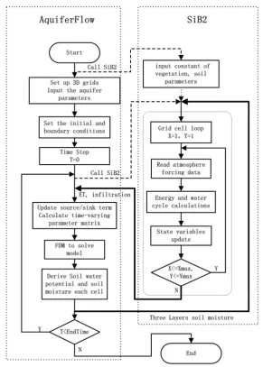
Fig. 1. The coupling between SiB2 and AquiferFlow in GWSiB. The bold solid lines with arrows indicate the direction of the transmission of variables, and the dashed lines with arrows indicate function calls.
2.3 Coupled model approach
As described above, the SiB2 and AquiferFlow models have strengths and weaknesses. Coupling the two models can overcome their weaknesses and more accurately simulate the water and energy cycles. In the study presented here, the two models were tightly coupled from the model codes, and a new model, named GWSiB, was developed. We will intro-duce the coupling mechanism in the following section.
In the coupled model, SiB2 simulates the energy balance, the vegetation root water uptake and the hydrologic processes above the ground surface, and AquiferFlow simulates water movement in the subsurface, including the saturated and un-saturated zones. Specifically, the SiB2 model is used to cal-culate the precipitation infiltration (Q1), the moisture
evapo-ration (Egs) and the transpiration (Ect) based on the energy
balance and the water balance. The calculated results are used as the sinks and sources (ε) and are input into Aquifer-Flow to calculate the groundwater potential (ψ). The ob-tained water potential is then used to calculate the ground-water movement in the model grids. The new groundground-water condition obtained is transferred back to SiB2 to complete the calculation cycle in one time step. A flowchart of the cou-pling procedure is illustrated in Fig. 1.
flexible layer structure than SiB2; consequently, the three subsurface layers in SiB2 are preserved, and the three top layers in AquiferFlow are set to be consistent with them. The infiltration and the soil evaporation are linked with the top layer of AquiferFlow, and the root zone uptake is linked with the second layer.
Although the surface runoff (R0) and the base flow (Q3)
are calculated on a vertical column in SiB2, the surface wa-ter convergence between cells is not taken into account in the coupled model. This simplification will not cause a sig-nificant deviation when the model is used in the middle or lower reaches of an arid or semi-arid basin, because there are almost no flow confluence processes in these regions. How-ever, if the model is used in the upper reach of a basin, the er-rors cannot be ignored. Wang et al. (2009) handled this prob-lem by coupling SiB2 with a geomorphology-based hydro-logical model (GBHM). In our study, the model validation and tests were performed in the middle reach of the Heihe River basin where the surface runoff is not the key hydrolog-ical process; consequently, the coupled model can be used here.
We now discuss how to handle the temporal discretization of the coupled models. LSMs usually use a time step of 1 h or less, because the energy and mass variables simulated by the LSM, such as the soil surface temperature, vary rapidly and vary significantly from day to night. However, the groundwa-ter head and flow vary more slowly; therefore, the time ingroundwa-ter- inter-vals used in GWMs are usually one day or longer. LSMs are more sensitive to the time resolution than GWMs and gener-ally cannot accept time intervals greater than 1 h. If the time step in an LSM is one day, the temporal fluctuations that oc-cur in hours will smooth out, generating significant calcula-tion errors and even making the simulacalcula-tion meaningless. A shorter time interval will not significantly affect the simula-tion accuracy of GWMs but will significantly reduce their computational efficiency.
Considering the time steps used in the two models, two al-ternative time coupling schemes are implemented in the cou-pled model. One scheme is to use the AquiferFlow time step (which is the same as that used in SiB2), which is set to be ei-ther 1 h or 30 min. The second scheme is to adopt a time step of one day in AquiferFlow, which is the time step normally used in the GWMs, while using a time step of 1 h in SiB2. The fluxes that are accumulated over one day in SiB2 are then exchanged with AquiferFlow. The first scheme has a higher precision but requires more computation; it is thus suitable for theoretical analysis or small-scale simulation. The sec-ond scheme greatly improves the computational efficiency and achieves acceptable calculation accuracy. This scheme is more suitable for large area simulation.
Both AquiferFlow and SiB2 use Richards equation as their control equations for soil water movement, but they adopt different parameterization schemes to describe the re-lationship between the unsaturated hydraulic conductivity (K) and the soil moisture potential (9). The Gardner and
Fireman (1958) method is used in AquiferFlow, and the Clapp and Hornberger (1978) scheme is used in SiB2. The different schemes would make a huge difference in the cal-culation of Richards equation. Because the different param-eter schemes can strongly affect the calculation results of Richards equation, a discontinuity would be created in the soil moisture at the two model communication times, espe-cially when using the second scheme, in which the water ac-cumulation is exchanged between the GWM and the LSM. To solve this problem, the Clapp and Hornberger (1978) soil moisture scheme used in SiB2 is introduced into the Aquifer-Flow model framework. In AquiferAquifer-Flow, the relative perme-ability (Kr) and the effective saturation (Se) are the two key
parameters for soil moisture movement and content. These two parameters are defined as fractions in AquiferFlow and are used to control the moisture movement in the unsaturated zone by adjusting the saturated hydraulic conductivity (Ks)
and the saturated soil water content (θs), which is
approx-imately equal to the porosity (φ). The parameters used in Clapp and Hornberger’s (1978) soil moisture scheme are also based on the saturated moisture potential (ψs) and the
satu-rated hydraulic conductivity (Ks); these equations can thus
be transformed to the AquiferFlow framework as
Se =W =
ψ
s ψ
B1
(10)
Kr=
ψ
s ψ
2BB+3
. (11)
Replacing the Kr and Se parameters of the AquiferFlow
model by Eqs. (10) and (11) makes the vadose zone parame-ters of AquiferFlow consistent with SiB2 and reduces the soil moisture discontinuities in the model at the time of coupling. After the GWSiB model is built, a sensitivity test about the key parameters of the model is performed, and the model validation is conducted based on the measured data of two observation stations. The model is then applied to the mid-dle reach of the Heihe River basin to test the applicability of the model on the regional scale. The following sections will describe the model validation in detail.
3 Model validation
40
1
2
Fig. 2. The synthetic model structure used in the sensitivity analysis of the GWSiB. The results 3
from the output cell located in the center of the platform are used for the analysis. 4
5
6
[image:7.595.131.470.63.206.2]7
Fig. 2. The synthetic model structure used in the sensitivity analysis of the GWSiB. The results from the output cell located in the center of the platform are used for the analysis.
the groundwater and the ET, a sensitivity test is performed prior to the model validation.
3.1 Sensitivity test
A synthetic domain is used to perform the sensitivity analy-sis of the GWSiB model. In this domain, there are two rivers separated by 200 m, with a platform located between the two rivers. The altitude of the platform is 1500 m, and its soil tex-tures are homogeneous and isotropic. The rivers can recharge the groundwater of the platform through lateral flow, so the river levels are generally representative of the groundwater level in the area. The synthetic domain is divided into an ar-ray of uniform vertical columns extending 3 columns wide parallel to the rivers and 10 columns long between the rivers; each column is 5 m wide and 20 m long (Fig. 2). In the verti-cal direction, the soil is divided into four layers representing the surface soil layer, the root layer, the deep soil layer and the phreatic aquifer layer, at 0.02, 0.48, 1.5, and 50 m, re-spectively. Consequently, the simulated domain forms a 120-element grid (10×3×4).
The model structure allows the groundwater level in the model to be easily controlled by directly changing the water level of the two rivers. The model structure can also incorpo-rate the characteristics of the lateral groundwater flow.
The forcing data used were measured at the Linze grass-land station (LZG) of the Heihe River basin at 17:00 LT (lo-cal time) on 12 August 2008; these data represent typi(lo-cal moderate-radiation atmospheric conditions in this arid re-gion. The forcing data are maintained constant throughout the simulation period in the sensitivity test.
The land cover of the simulated area is assumed to be grassland. The vegetation parameters used are the default pa-rameters for the “short vegetation/C4 grassland” vegetation type, which is one of the nine types of vegetation derived from Sellers et al. (1996a) that are defined in SiB2. The leaf area index (LAI) used to represent vegetation growth is kept at a constant value of 2 during the simulation period.
41
1
2
Fig. 3. Simulated ET results at different groundwater depth (GWD) conditions. 3
4
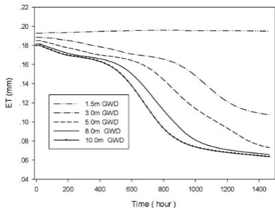
Fig. 3. Simulated ET results at different groundwater depth (GWD) conditions.
In the model, the two rivers are defined as fixed head boundaries. The other groundwater boundaries are defined using the no-flow condition. The river levels, the soil tex-ture and the groundwater hydraulic parameters are specified according to the sensitivity tests described in detail in the fol-lowing. The first time-coupling scheme described in Sect. 2.3 is used in the sensitivity test, and the time step is set to 1 h. The simulation period is 1488 h.
Using the model, the impact of the groundwater depth on the ET is first analyzed. Five groundwater depths are simu-lated: 1.5, 3.0, 5.0, 8.0, and 10.0 m (corresponding to river levels of 1498.5, 1497.0, 1495.0, 1492.0, and 1490.0 m, re-spectively). In this experiment, the soil texture is set to 30 % clay, 30 % silt, and 40 % sand. The results from the cell lo-cated in the center of the platform are used for the analysis. The analysis results are shown in Fig. 3.
[image:7.595.325.526.260.412.2]surface and the root soil layer by capillary action, and the reduction in the surface water limits ET. The simulated ET also decreases continuously with time, except in the case of the 1.5 m groundwater depth. We believe this is due to the ve-locity of groundwater flow, which includes the veve-locity of the lateral flow and the vertical flow. When the water lost in ET is greater than the water gained through groundwater recharge, the soil gradually dries, and ET decreases. However, there is a sufficient water supply in the case of the 1.5 m ground-water depth, so ET does not significantly decline during the simulation period.
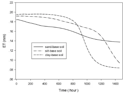
This analysis shows that the groundwater flow can sig-nificantly affect ET. In the GWSiB model, the flow char-acteristics of the groundwater are determined by the soil texture and calculated using an empirical formula (Yang et al., 2005). Consequently, in the second experiment, the ef-fect of different soil textures on the ET is analyzed. Three soil texture types, including sand-based soil (clay: 20 %, silt: 20 %, sand: 60 %), silt-based soil (clay: 20 %, silt: 60 %, sand: 20 %), and clay-based soil (clay: 60 %, silt: 20 %, sand: 20 %), are used in this experiment. The rele-vant parameters defined by Clapp and Hornberger (1978) areKs= 0.66 m day−1, 8s= 0.12 m, and B= 6.09 for
sand-based soil; Ks= 0.16 m day−1, 8s= 0.41 m, and B= 6.09
for silt-based soil; andKs= 0.16 m day−1,8s= 0.41 m, and B= 12.45 for clay-based soil. In this experiment, the ground-water level is set to 3 m. The results are shown in Fig. 4.
Figure 4 shows that the hydraulic characteristics of the groundwater have a significant effect on ET. The slope of the decrease in ET of the sand-based soil is less than the other soil types. This is because the sand-based soil has a higher hydraulic conductivity than the other soil types, and the wa-ter in the soil that is lost by ET can be recovered quickly. In contrast, the clay-based and silt-based soils have greater capillary action (i.e., these soil types have a higher saturation moisture potential). These soil types can provide more wa-ter to the ET process early in the simulation, but, as the soil moisture decreases, the water in the soil cannot be quickly replenished, and the rate of ET decreases rapidly.
3.2 Model validation
Based on the sensitivity analysis model, the GWSiB is vali-dated at the Linze grassland station (LZG) and the National Observatory on Climatology at Zhangye (ZYNOC), which represent shallow and deep groundwater conditions, respec-tively. The measured data from the two stations, including atmospheric driving data, vegetation data, soil textures and groundwater levels, are input to the model as the true value. The vegetation parameters are calibrated for each station be-fore the model validation is performed. The detailed process is as follows.
42
1
2
Fig. 4. Simulated ET results at different soil texture conditions. 3
4
Fig. 4. Simulated ET results at different soil texture conditions.
3.2.1 Validation of the model for the Linze grassland station (LZG)
The LZG is located in the middle reach of the Heihe River basin in the northwest of China. The longitude is 100.07◦E, and the latitude is 39.25◦N. The land cover in the LZG is mainly wetland, grassland and salinized meadow. An auto-matic meteorological station (AMS) built by the Watershed Allied Telemetry Experimental Research (WATER) project (Li et al., 2009) in the LZG was used for observations from 1 October 2007 to 27 October 2008. The AMS provides all the necessary atmospheric forcing data for our modeling study. Although there is no direct measurement of the latent heat at the LZG station, it can be obtained from the sensible heat by the energy balance equation:
λE =Rn−H −G (12)
whereλE is the latent heat (W m−2); λ is the heat of va-porization (J kg−1);Eis the ET (m);Rnis the net radiation
(W m−2), equal to the difference of the downward radiation and the upward radiation, which can be obtained from the at-mospheric forcing data; andH is the sensible heat. In the WATER experiment, a large-aperture scintillometer (LAS) flux system was used from 19 May 2008 to 27 August 2008 to obtain the sensible heat data for the model.Gis the ground heat flux (W m−2) and is assumed to be proportional to the net radiation (Su, 2002):
G=Rn·[0c+(1−fc)·(0s −0c)] (13)
where0c= 0.05 for a full vegetation canopy,0s= 0.315 for
bare soil, andfcis the fractional canopy coverage, which is
set to 0.81 based on observations in the LZG. The latent heat of the LZG is calculated according to a variety of observa-tional data and the energy balance equation; the ET is then deduced based on the latent heat.
[image:8.595.325.527.62.215.2]LZG Short 0.81 0.3 0.03 0.105 0.58 310 280 vegetation/
C4 grassland
ZYNOC Broadleaf 0.01 0.2 0.03 0.1 0.45 313 283
shrub and bare soil
43 1
2
Fig. 5. The measured evapotranspiration, the GWSiB-simulated evapotranspiration, and the 3
SiB2-simulated evapotranspiration for the Linze grassland station from May 19, 2008 to August 4
27, 2008. The data in the shadowed part of the graph are used for the model parameter calibration, 5
while the other data are used for the model validation. 6
7
Fig. 5. The measured evapotranspiration, the GWSiB-simulated evapotranspiration, and the SiB2-simulated evapotranspiration for the Linze grassland station from 19 May 2008 to 27 August 2008. The data in the shadowed part of the graph are used for the model parameter calibration, while the other data are used for the model validation.
varies between 1.2 and 1.9 m during the simulation period. The vegetation type used in the LZG model is “C3 grass-land”, and the parameters from Sellers et al. (1996a) for this vegetation type are calibrated according to the ET measured in the LZG from 19 May to 1 July 2008. The parameters used in the model are listed in Table 1. In the GWSiB model, the LAI has often been used to characterize the vegetation growth process. The LAI data for the LZG were obtained from MODIS global LAI and FPAR (fraction of photosyn-thetically active radiation) products (MCD15A3) with a 4-day time resolution and a 1-km spatial resolution. These data were revised according to observation and interpolated to the 1-h time resolution used in the model. The LAI varies from 2.1 to 3.4 during the simulation period.
The same model structure as in the sensitivity test is used in the model validation, including the same spatial structure and the same time step. The data described above are used as the input to the GWSiB model to simulate the energy and wa-ter cycles of the LZG from 19 May 2008 to 27 August 2008.
44
1
Fig. 6. A scatter plot comparing the GWSiB-simulated and the SiB2-simulated evapotranspiration 2
with the measured evapotranspiration in the Linze grassland station. 3
4
5
6
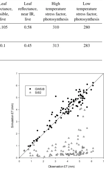
Fig. 6. A scatter plot comparing the GWSiB-simulated and the SiB2-simulated evapotranspiration with the measured evapotranspi-ration in the Linze grassland station.
[image:9.595.306.526.83.441.2] [image:9.595.71.386.83.391.2]45
2
Fig. 7.The measured evapotranspiration, the GWSiB-simulated evapotranspiration, and the 3
SiB2-simulated evapotranspiration for the National Observatory on Climatology station at 4
Zhangye from June 28, 2008 to August 22, 2008. The data in the shadowed part of the graph are 5
used for the model parameter calibration, while the other data are used for the model validation. 6
7
8
Fig. 7. The measured evapotranspiration, the GWSiB-simulated evapotranspiration, and the SiB2-simulated evapotranspiration for the National Observatory on Climatology station at Zhangye from 28 June 2008 to 22 August 2008. The data in the shadowed part of the graph are used for the model parameter calibration, while the other data are used for the model validation.
mean value from the SiB2 model is 0.76 mm per day, and the MRE is 80.7 %.
The GWSiB model can provide a more realistic simulation than the SiB2 model, because the movement of the ground-water is taken into account in the GWSiB model but not in the SiB2 model. The lateral flow of groundwater causes groundwater accumulation in the shallow-water region and raises the groundwater level. The saturated groundwater sup-plies water to the soil near the ground surface by capillary action, leading to greater ET at the land surface in the LZG. Compared with the GWSiB model, the SiB2 model is a ver-tical 1-D model that cannot model the process of ground-water recharge by lateral ground-water movement; consequently, the soil water moisture of the land surface is underestimated, and the lower soil moisture reduces the ET observed in the SiB2 model.
3.2.2 Validation of the model for the National Observatory on Climatology at Zhangye
The National Observatory on Climatology at Zhangye is one of China’s national climatology stations. The station is lo-cated in the middle reach of the Heihe River basin at a lon-gitude of 100.28◦E and a latitude of 39.08◦N. The ZYNOC has a Gobi landscape. Comprehensive atmospheric and heat flux data are measured in the ZYNOC that can support the validation of the model for the ZYNOC. ET data in the form of the latent heat were obtained from 28 June 2008 to 22 Au-gust 2008. Some of these data were removed because the data quality was poor, and only 41 days of latent heat observations are used for the model validation.
Of the nine vegetation types defined in the SiB2 model, the “broadleaf shrubs with bare soil” type is chosen as the closest to the actual conditions of the ZYNOC. The parameters from
46
1
Fig. 8. A scatter plot comparing the GWSiB-simulated and the SiB2-simulated evapotranspiration 2
with the measured evapotranspiration in the National Observatory on Climatology station at 3
Zhangye. 4
Fig. 8. A scatter plot comparing the GWSiB-simulated and the SiB2-simulated evapotranspiration with the measured evapotran-spiration in the National Observatory on Climatology station at Zhangye.
Sellers et al. (1996a) for this vegetation type are calibrated according to the ET measurements. The typical soil textures of the ZYNOC obtained from field measurements are 23 % clay, 30 % sand and 47 % silt. The groundwater level data come from a well approximately 2 km from ZYNOC. The variation of the groundwater depth is not significant during the simulation period; the depth varies from 25.4 to 26.2 m. The groundwater levels are used as fixed-head boundary con-ditions in the model. The LAI data are obtained from the MODIS products (MCD15A3), in a manner similar to the validation of the LZG. The LAI of the ZYNOC increases from 0.1 to 0.4 during the simulation period.
The setup of the model for the ZYNOC validation is the same as that used for the LZG validation. The simulation pe-riod is from 28 June 2008 to 22 August 2008. The ET data from 28 June to 21 July are used to calibrate the vegetation parameters of the model. The parameters that are held con-stant throughout the simulation period are listed in Table 1. The remainder of the simulation period is used to validate the model. The ET processes are simulated in the SiB2 model using the same conditions, except that the groundwater level is not considered in the SiB2 model. The simulation results from the two models are shown in Figs. 7 and 8.
[image:10.595.326.527.62.261.2] [image:10.595.67.268.63.216.2]47
[image:11.595.123.467.60.361.2]1
Fig. 9. The location of the study area in the middle reach of the Heihe River basin and the model 2
grid structure. 3
4
5
6
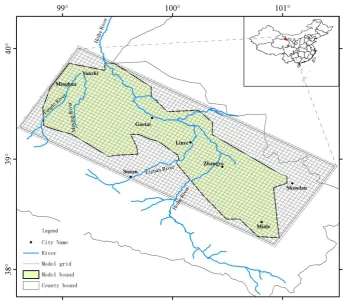
Fig. 9. The location of the study area in the middle reach of the Heihe River basin and the model grid structure.
from the SiB2 model is 0.69 mm per day, and the MRE is 4.7 %.
We believe that the groundwater level and the lateral flow of the groundwater have a small effect on the energy and water cycles on the land surface because the groundwater is deep (approximately 26 m below ground surface). In the thick vadose zone, water movement occurs primarily in the vertical dimension. Both the SiB2 and the GWSiB models can simulate this process adequately, and they provide simi-lar and realistic results. The GWSiB and SiB2 results never-theless show some minor differences; e.g., the variations in the simulated ET are greater in the SiB2 model than in the GWSiB model, and the SiB2 model tends to produce larger or smaller extreme values. We believe that the difference in the results can be attributed to the difference in the two model structures.
4 Regional test of the model
The validation of the GWSiB model in the shallow ground-water site (LZG) and the deep groundground-water site (ZYNOC) demonstrates the adequacy of the model. However, the water cycle can usually only be understood comprehensively on a regional scale. Because the GWSiB model is fundamentally a 3-D model, it has the ability to simulate regional water and
energy cycles. In the following, the GWSiB is applied in the middle reach of the Heihe River basin to test the simulation capabilities of the model in the region.
4.1 Study area
The middle reach of the Heihe River basin is an arid in-land river basin located in northwestern China. In this basin, an integral groundwater cell, which is hydrogeologically de-scribed as the Zhangye basin, is selected as the study area. The latitude of the study area ranges from 38.7◦N to 39.8◦N,
the longitude from 98.5◦E to 102◦E, and the total area is
4.2 Model settings
The study area is uniformly discretized into 79 rows and 32 columns horizontally, and each numerical cell has dimen-sions of 3 km×3 km. In the vertical direction, the soil be-low the ground surface is divided into six layers. The upper three layers correspond to the soil layers of the SiB2 model and represent the surface soil, the soil root, and the deeper soil layers. The thickness of these soil layers is set to 0.02, 0.48, and 1.5 m, respectively, according to the average con-ditions of the soils in the middle reach of the Heihe River basin. The lower three layers are used to describe the hy-drogeologic structure in the study area, representing the un-confined aquifer, the aquitard and the un-confined aquifer. The thicknesses of the lower three layers are determined by the interpretation of the logging data obtained from 108 bore-holes in the region, as proposed by Zhou et al. (1990). The study area contains a total of 15 168 (79×32×6) cells, as shown in Fig. 9.
The topography of the study area is determined from 90-m resolution digital elevation 90-model (DEM) data obtained from the Shuttle Radar Topography Mission (SRTM) and up-scaled to 3-km resolution. The initial GWT distribution in the study area is obtained by the interpolation of GWT mea-surements conducted in December 2003 from 36 observation wells in the study area. Any GWT positions not available from the measurements are determined from the relevant lit-erature (Su, 2005; Hu et al., 2007; Wen et al., 2007; Zhou et al., 2011). The initial GWT data show that the main di-rection of the groundwater flow of the middle reach of the Heihe River basin is from south to north and is roughly consistent with the river flow direction. The GWT is lower in the north of the study area, where the groundwater dis-charges to the river. The boundary conditions and the satu-rated hydraulic conductivity (Ks) of the model were initially
assigned values according to previous study results from the Heihe River basin (Su, 2005; Hu et al., 2007; Wen et al., 2007; Ding et al., 2009; Zhou et al., 2011). Later, these pa-rameters were optimized through trial-and-error calculations using GWT data obtained in January 2008. Ultimately, the boundary conditions of the model are set as fixed-flow condi-tions: the southern boundary has 1.62×10⁸m3water inflow every year; the northern boundary has 0.37×10⁸m3a−1 wa-ter inflow; and the weswa-tern and easwa-tern boundaries have a total of 0.08×10⁸m3a−1water inflow. These water inflows were allocated to each of the active cells of the boundary grid in the model. The saturated hydraulic conductivity (Ks) field
in the study area was divided into 24 sub-regions, with val-ues ranging from 0.5 m d−1to 20 m d−1. The distribution of the specific storage (Ss) was represented by 10 sub-regions,
with values ranging from 0.003 m−1 to 0.17 m−1. The wa-ter potential paramewa-ters of the unsaturated zone were dewa-ter- deter-mined according to the soil texture. The parameter values for the soil characteristics used in this study were obtained through the analysis of the Chinese dataset of the multi-layer
soil-particle size distribution, which has a 1-km resolution (Shangguan et al., 2012).
The atmospheric data used in the model, including the incident solar radiation, incident longwave radiation, wind speed, air pressure, vapor pressure, air temperature, and pre-cipitation, are taken from the Global Land Data Assimilation System (GLDAS) project (Rodell et al., 2004). The spatial resolution of the original data is 25 km, and the temporal res-olution is 3 h. The data are interpolated to a spatial resres-olution of 3 km and a temporal resolution of 1 h to fit the resolution of the coupled model. The temporal interpolations of the data were performed using a statistical method provided by the Global Soil Wetness Project 2 (GSWP2) (for the precipita-tion data) and the cubic spline method (Dai et al., 2003) (for other data). The high-resolution meteorological interpolation model MicroMet (Liston and Elder, 2006) is used in the spa-tial interpolation of the data. These data are used in all of the model cells except those cells where an AMS is located. In those cells, the interpolated atmospheric data are replaced by the measured data.
The land cover data used in the model are derived from the Multi-source Integrated Chinese Land Cover (MICL Cover) data (Ran et al., 2012). The International Geosphere-Biosphere Programme (IGBP) land cover classification sys-tem is used in the MICL Cover data, and the land surface is classified into 17 types. In this study, the 17 types are grouped into nine types corresponding to the vegetation clas-sifications of the SiB2 model (Sellers et al., 1996b). The parameters of each vegetation type defined by Sellers et al. (1996a) are calibrated according to the measured ET data from this study.
There is a considerable amount of farmland in the study area, and the energy and water cycles are affected by the irri-gation. In this model, the irrigation is modeled by sink terms added to the groundwater system on the grid cells at which the vegetation type of cells is defined as “agricultural”. The irrigation data used in the model come from the local admin-istrative department of agriculture.
The time-dependent vegetation parameters used in the coupled model were obtained from satellite data. The level-4 combined (Terra and Aqua) MODIS global LAI and FPAR products (MCD15A3), which are provided every 4 days at a resolution of 1 km, are linearly interpolated to a temporal scale of 1 h and are resampled to a spatial resolution of 3 km for the coupled model.
48
2
Fig. 10. The observed and simulated groundwater table (GWT) of the study area in December 3
2008. The observed GWT within the scope of the 36 wells (the interpolation range) is obtained by 4
interpolation; the rest of the GWT in the study area is obtained by extrapolation. 5
6
[image:13.595.124.467.60.291.2]7
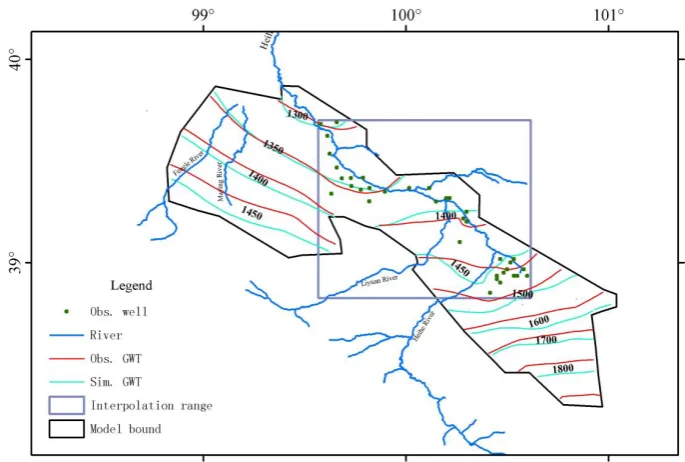
Fig. 10. The observed and simulated groundwater table (GWT) of the study area in December 2008. The observed GWT within the scope of the 36 wells (the interpolation range) is obtained by interpolation; the rest of the GWT in the study area is obtained by extrapolation.
Because the groundwater flow equation is highly nonlin-ear, the convergence of the groundwater model needs care-ful adjustment of the slover. In this study, the model con-vergence was implemented through the adjustment of the relaxation factor, the number of iterations, and the conver-gence criterium, which were set to 1.3, 10 000, and 0.001 m, respectively.
The initial conditions of the model, such as the soil mois-ture, surface temperamois-ture, canopy temperature and other vari-ables, are determined according to the general conditions in the middle reach of the Heihe River basin in winter. The ini-tial conditions are specified in the coupled model for 1 uary 2004. The model is run for 4 yr as a spin-up from 1 Jan-uary 2004 to 1 JanJan-uary 2008 to ensure that the model is ini-tially in equilibrium. The simulated values at the end of the spin-up period (1 January 2008) are treated as the initial con-ditions of the simulation period for the coupled model. 4.3 Analysis of the model results
Using the GWSiB model of the middle reach of the Heihe River basin, the energy budget and the water movements in this region were simulated from 1 January to 31 Decem-ber 2008. We analyzed the results of the model to test the model on the regional scale. First, the simulated GWT data from 20 December 2008 are compared with the measured GWT data for the same day obtained from the interpolation of the data from the 36 observation wells. The results are shown in Fig. 10.
The simulation results and the measurements agree well (Fig. 10) except on the west side of the study area, where
the groundwater depth is greater than 100 m and there are few groundwater observation wells. The initial GWT data for these regions are taken from the existing literature (Su, 2005; Wen et al., 2007), and the measured data for these re-gions are extrapolated from the 36 observation wells. We be-lieve the uncertainty of the GWT data for these areas is the main reason for the simulation errors. Additionally, in the upper section of the Heihe River, the simulated GWT results are higher than the measured GWT data (e.g., at the 1450 m GWT) in Fig. 10. This is because the upper section of the Heihe River is considered to be the region of surface water recharge to the groundwater in the coupled model. The sig-nificant water infiltration in this region and the partial GWT increase are simulated in the model, but this change is not caught in the measurements because there are few observed wells in this region to provide data for the GWT interpo-lation. In general, the GWSiB simulation produces a good model of the groundwater conditions of the middle reach of the Heihe River basin, and the GWSiB model can provide a continuous and time-varying depiction of the impact of the groundwater on the land surface energy and water cycles.
49
1
[image:14.595.58.542.59.239.2]2
Fig. 11. Evapotranspiration calculated by remote sensing (a) and simulated by the GWSiB model 3
(b) in the middle reach of the Heihe River basin at 15:00 local time on August 8, 2008. The map (a) 4
is derived from Li et al. (2011). 5
6
49
2
Fig. 11. Evapotranspiration calculated by remote sensing (a) and simulated by the GWSiB model 3
(b) in the middle reach of the Heihe River basin at 15:00 local time on August 8, 2008. The map (a) 4
is derived from Li et al. (2011). 5
6
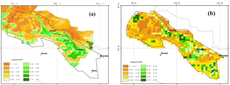
Fig. 11. Evapotranspiration calculated by remote sensing (a) and simulated by the GWSiB model (b) in the middle reach of the Heihe River basin at 15:00 LT on 8 August 2008. The map (a) is derived from Li et al. (2012).
The results of the model simulation and the remote sens-ing calculation have a very similar spatial distribution, and both show the ET distribution characteristics of the middle reach of the Heihe River basin. In this region, the banks of the Heihe River and the irrigated area have greater ET because the river recharges the groundwater through lateral flow and raises the groundwater levels of the banks while the irrigation increases the soil moisture of the irrigated area. The average ET in the study area determined from the model simulation is 0.24 mm, and the value calculated from the remote sens-ing data is 0.31 mm. There is a 23 % MRE between the two values. However, some details are not consistent between the two results. The main reason for the inconsistency, besides the error caused by the remote sensing terms, is the model un-certainties, including uncertainty in the meteorological driv-ing data, the land cover data, the soil texture data, the ground-water data, and the grid structure of the model.
On the whole, the GWSiB model can simulate regional energy and water cycles, although there are some errors. In this test, the GWSiB model achieves an acceptable regional ET simulation of the middle reach of the Heihe River basin both in terms of absolute values as spatial distribution.
5 Discussion and conclusions
LSMs can describe the land surface energy and water cy-cles well, but the water movement in the subsurface is over-simplified, and the movement of saturated groundwater is ig-nored. Conversely, GWMs can describe the dynamic move-ment of subsurface water, but they cannot simulate the phys-ical mechanisms of ET, which is an important component of the water cycle because this process involves the energy cy-cle and the biological processes. Coupling the two types of models can effectively overcome their respective shortcom-ings, and, by linking the energy and water cycles together,
these processes can be simulated more comprehensively and potentially more accurately.
In this study, a 3-D dynamic groundwater model, Aquifer-Flow, and a typical land surface model, SiB2, are fully cou-pled. In the coupling scheme, infiltration, evaporation and transpiration, which are simulated by the SiB2 model, are used as inputs to the AquiferFlow model, and the soil mois-ture values calculated by AquiferFlow are used in SiB2. In the sensitivity analysis of the coupled model, the effects of the groundwater level and the hydraulic parameters of the groundwater on the energy and water cycles are analyzed. The excellent performance of the GWSiB model in the LZG and ZYNOC validation studies demonstrates that the coupled model has the proper structure. Additionally, the case study of the middle reach of the Heihe River basin demonstrates the ability of the GWSiB model to simulate regional-scale dynamics.
can describe the energy and water processes as a system, and the model can be widely used in the study of Earth science.
From our study, the following four conclusions can be obtained.
1. The groundwater depth can significantly affect the ET on the land surface; the ET increases as the ground-water depth decreases. Additionally, the groundground-water hydraulic parameters and the soil structure can affect ET through the vertical and lateral movement of the groundwater.
2. In a shallow groundwater depth zone, the GWSiB model, which incorporates the groundwater movement, simulates the ET process on the land surface more ac-curately than the SiB2 model, in which the groundwater movement is not simulated. The ET will be underesti-mated if the groundwater movement is ignored in this region.
3. The interaction of the groundwater and the land surface processes is weak in zones of large depth to groundwa-ter, and the subsurface water movement is dominated by vertical movement under these conditions. The GWSiB model produces results similar to the SiB2 model, and each of the models can simulate the ET process in this region well.
4. The GWSiB model can simulate regional energy and water cycles. The GWSiB simulation accurately mod-els the middle reach of the Heihe River basin. The accu-racy not only depends on the correctness of the model structure but is also directly affected by the model data. In summary, the coupling of the groundwater and land sur-face models allows the land sursur-face and subsursur-face processes to be simulated as a system, and the coupled model can depict the interaction of the groundwater and the energy and water movement on the land surface. This improves the simulation of the energy and water cycles.
Although a coupled model was developed in this study, some the energy and water processes, such as surface water processes, water resource allocation, and soil freezing and thawing processes, are not considered in the model. Addi-tionally, the validation of the GWSiB model is limited by the shortage of available data. Further validation and improve-ment of the coupled model will be the primary thrust of fu-ture studies.
two reviewers for improving the quality of this manuscript.
Edited by: H. Cloke
References
Baker, I., Denning, A. S., Hanan, N., Prihodko, L., Uliasz, M., Vi-dale, P. L., Davis, K., and Bakwin, P.: Simulated and observed fluxes of sensible and latent heat and CO2 at the WLEF-TV tower using SiB2.5, Global Change Biol., 9, 1262–1277, 2003. Clapp, R. B. and Hornberger, G. M.: Empirical equations for
some soil hydraulic properties, Water Resour. Res., 14, 601–604, doi:10.1029/WR014i004p00601, 1978.
Colello, G. D., Grivet, C., Sellers, P. J., and Berry, J. A.: Modeling of energy, water, and CO2flux in a temperate grassland ecosystem
with SiB2: May–October 1987, J. Atmos. Sci., 55, 1141–1169, 1998.
Cosby, B. J., Hornberger, G. M., Clapp, R. B., and Ginn, T. R.: A Statistical Exploration of the Relationships of Soil-Moisture Characteristics to the Physical-Properties of Soils, Water Resour. Res., 20, 682–690, 1984.
Dai, Y., Zeng, X., Dickinson, R. E., Baker, I., Bonan, G. B., Bosilovich, M. G., Denning, A. S., Dirmeyer, P. A., Houser, P. R., Niu, G., Oleson, K. W., Schlosser, C. A., and Yang, Z.-L.: The Common Land Model, B. Am. Meteorol. Soc., 84, 1013– 1023, doi:10.1175/bams-84-8-1013, 2003.
Ding, H.-W., Xu, D.-L., Zhao, Y.-P., and Yang, J.-J.: Dynamic char-acteristic and forecast of spring water in the middle reaches of Heihe River trunk stream area in Gansu Province, Arid Land Ge-ogr., 32, 726–732, 2009.
Fan, Y., Miguez-Macho, G., Weaver, C. P., Walko, R., and Robock, A.: Incorporating water table dynamics in climate modeling: 1. Water table observations and equilibrium wa-ter table simulations, J. Geophys. Res.-Atmos., 112, D10125, doi:10.1029/2006jd008111, 2007.
Gao, Z. Q., Chae, N., Kim, J., Hong, J. Y., Choi, T., and Lee, H.: Modeling of surface energy partitioning, surface temperature, and soil wetness in the Tibetan prairie using the Simple Bio-sphere Model 2 (SiB2), J. Geophys. Res.-Atmos., 109, D06102 doi:10.1029/2003jd004089, 2004.
Gardner, W. R. and Fireman, M.: Laboratory Studies of Evaporation From Soil Columns in the Presence of A Water Table, Soil Sci., 85, 244–249, 1958.
Gedney, N. and Cox, P. M.: The Sensitivity of Global Climate Model Simulations to the Representation of Soil Moisture Het-erogeneity, J. Hydrometeorol., 4, 1265–1275, doi:10.1175/1525-7541(2003)004<1265:tsogcm>2.0.co;2, 2003.
Holt, T. R., Niyogi, D., Chen, F., Manning, K., LeMone, M. A., and Qureshi, A.: Effect of land-atmosphere interactions on the IHOP 24–25 May 2002 convection case, Mon. Weather Rev., 134, 113– 133, doi:10.1175/mwr3057.1, 2006.
Hu, L.-T., Chen, C.-X., Jiao, J. J., and Wang, Z.-J.: Simulated groundwater interaction with rivers and springs in the Heihe river basin, Hydrol. Process., 21, 2794-2806, doi:10.1002/hyp.6497, 2007.
Kollet, S. J. and Maxwell, R. M.: Integrated surface-groundwater flow modeling: A free-surface overland flow boundary condition in a parallel groundwater flow model, Adv. Water Resour., 29, 945–958, doi:10.1016/j.advwatres.2005.08.006, 2006.
Kollet, S. J. and Maxwell, R. M.: Capturing the influence of ground-water dynamics on land surface processes using an integrated, distributed watershed model, Water Resour. Res., 44, W02402, doi:10.1029/2007wr006004, 2008.
Li, X. and Koike, T.: Frozen soil parameterization in SiB2 and its validation with GAME-Tibet observations, Cold Reg. Sci. Tech-nol., 36, 165–182, 2003.
Li, X., Li, X. W., Li, Z. Y., Ma, M. G., Wang, J., Xiao, Q., Liu, Q., Che, T., Chen, E. X., Yan, G. J., Hu, Z. Y., Zhang, L. X., Chu, R. Z., Su, P. X., Liu, Q. H., Liu, S. M., Wang, J. D., Niu, Z., Chen, Y., Jin, R., Wang, W. Z., Ran, Y. H., Xin, X. Z., and Ren, H. Z.: Watershed Allied Telemetry Experimental Research, J. Geophys. Res.-Atmos., 114, D22103, doi:10.1029/2008jd011590, 2009. Li, X., Lu, L., Yang, W., and Cheng, G.: Estimation of
evapotran-spiration in an arid region by remote sensing – A case study in the middle reaches of the Heihe River Basin, Int. J. Appl. Earth Obs. Geoinf., 17, 85–93, doi:10.1016/j.jag.2011.09.008, 2012. Liang, X., Xie, Z. H., and Huang, M. Y.: A new
parameter-ization for surface and groundwater interactions and its im-pact on water budgets with the variable infiltration capacity (VIC) land surface model, J. Geophys. Res.-Atmos., 108, 8613, doi:10.1029/2002jd003090, 2003.
Liston, G. E. and Elder, K.: A meteorological distribution system for high-resolution terrestrial modeling (MicroMet), J. Hydrom-eteorol., 7, 217–234, 2006.
Maxwell, R. M. and Miller, N. L.: Development of a coupled land surface and groundwater model, J. Hydrometeorol., 6, 233–247, doi:10.1175/jhm422.1, 2005.
Maxwell, R. M., Chow, F. K., and Kollet, S. J.: The groundwater-land-surface-atmosphere connection: Soil mois-ture effects on the atmospheric boundary layer in fully-coupled simulations, Adv. Water Resour., 30, 2447–2466, doi:10.1016/j.advwatres.2007.05.018, 2007.
Maxwell, R. M., Lundquist, J. K., Mirocha, J. D., Smith, S. G., Woodward, C. S., and Tompson, A. F. B.: Development of a Cou-pled Groundwater-Atmosphere Model, Mon. Weather Rev., 139, 96–116, doi:10.1175/2010mwr3392.1, 2011.
McDonald, M. G. and Harbaugh, A. W.: A modular three dimen-sional finite difference ground-water flow model: US Geological Survey Techniques of Water Resources Investigations, US Geo-logical Survey, Denver, Colorado, 586 pp., 1998.
Niu, G. Y., Yang, Z. L., Dickinson, R. E., Gulden, L. E., and Su, H.: Development of a simple groundwater model for use in cli-mate models and evaluation with Gravity Recovery and Cli-mate Experiment data, J. Geophys. Res.-Atmos., 112, D07103, doi:10.1029/2006jd007522, 2007.
Ran, Y., Li, X., Lu, L., and Li, Z.: Large-scale land cover map-ping with the integration of multi-source information based on the Dempster–Shafer theory, Int. J. Geogr. Inf. Sci., 26, 169–191, 2012.
Rodell, M., Houser, P. R., Jambor, U., Gottschalck, J., Mitchell, K., Meng, C. J., Arsenault, K., Cosgrove, B., Radakovich, J., Bosilovich, M., Entin, J. K., Walker, J. P., Lohmann, D., and Toll, D.: The Global Land Data Assimilation System, B. Am. Meteo-rol. Soc., 85, 381–394, doi:10.1175/bams-85-3-381, 2004. Sellers, P. J., Mintz, Y., Sud, Y. C., and Dalcher, A.: A simple
bio-sphere model (sib) for use within general-circulation models, J. Atmos. Sci., 43, 505–531, 1986.
Sellers, P. J., Shuttleworth, W. J., Dorman, J. L., Dalcher, A., and Roberts, J. M.: Calibrating the simple biosphere model for ama-zonian tropical forest using field and remote-sensing data, 1. av-erage calibration with field data, J. Appl. Meteorol., 28, 727–759, 1989.
Sellers, P. J., Los, S. O., Tucker, C. J., Justice, C. O., Dazlich, D. A., Collatz, G. J., and Randall, D. A.: A revised land surface param-eterization (SiB2) for atmospheric GCMs, 2. The generation of global fields of terrestrial biophysical parameters from satellite data, J. Climate, 9, 706–737, 1996a.
Sellers, P. J., Randall, D. A., Collatz, G. J., Berry, J. A., Field, C. B., Dazlich, D. A., Zhang, C., Collelo, G. D., and Bounoua, L.: A revised land surface parameterization (SiB2) for atmospheric GCMs, 1. Model formulation, J. Climate, 9, 676–705, 1996b. Sen, O. L., Shuttleworth, W. J., and Yang, Z. L.: Comparative
evalu-ation of BATS2, BATS, and SiB2 with Amazon data, J. Hydrom-eteorol., 1, 135–153, 2000.
Shangguan, W., Dai, Y., Liu, B., Ye, A., and Yuan, H.: A soil particle-size distribution dataset for regional land and climate modelling in China, Geoderma, 171–172, 85–91, doi:10.1016/j.geoderma.2011.01.013, 2012.
Soylu, M. E., Istanbulluoglu, E., Lenters, J. D., and Wang, T.: Quan-tifying the impact of groundwater depth on evapotranspiration in a semi-arid grassland region, Hydrol. Earth Syst. Sci., 15, 787– 806, doi:10.5194/hess-15-787-2011, 2011
Su, J.: Groundwater flow modeling and sustainable utilization of water resources in Zhangye Basin of Heihe River Basin, North-western China PHD, Cold and Arid Regions Environmental and Engineering Research Institute, Chinese Academy of Sciences, Beijing, China, 2005.
Su, Z.: The Surface Energy Balance System (SEBS) for estima-tion of turbulent heat fluxes, Hydrol. Earth Syst. Sci., 6, 85–100, doi:10.5194/hess-6-85-2002, 2002.
Tian, X. J., Xie, Z. H., Zhang, S. L., and Liang, M. L.: A subsurface runoff parameterization with water storage and recharge based on the Boussinesq-Storage Equation for a Land Surface Model, Sci. China Ser. D, 49, 622–631, doi:10.1007/s11430-006-0622-z, 2006.
Twarakavi, N. K. C., Simunek, J., and Seo, S.: Evaluating interac-tions between groundwater and vadose zone using the HYDRUS-based flow package for MODFLOW, Vadose Zone J., 7, 757– 768, doi:10.2136/vzj2007.0082, 2008.
periments (SGP97 and SGP99), J. Geophys. Res.-Atmos., 114, D08107, doi:10.1029/2008jd010800, 2009.
Wang, X. S.: AquiferFlow: A finite difference variable saturation three-dimensional aquifer groundwater flow model, China Uni-versity of Geosciences (Beijing), Beijing, China, 2007. Wang, X.-S., Ma, M.-G., Li, X., Zhao, J., Dong, P., and Zhou,
J.: Groundwater response to leakage of surface water through a thick vadose zone in the middle reaches area of Heihe River Basin, in China, Hydrol. Earth Syst. Sci., 14, 639–650, doi:10.5194/hess-14-639-2010, 2010.
Wen, X. H., Wu, Y. Q., Lee, L. J. E., Su, J. P., and Wu, J.: Groundwa-ter flow modeling in the zhangye basin, northwesGroundwa-tern china, En-viron. Geol., 53, 77–84, doi:10.1007/s00254-006-0620-7, 2007. Yang, K., Koike, T., Ye, B. S., and Bastidas, L.: Inverse analysis
of the role of soil vertical heterogeneity in controlling surface soil state and energy partition, J. Geophys. Res.-Atmos., 110, D08101, doi:10.1029/2004jd005500, 2005.
sour., 25, 221–238, 2002.
Yuan, X., Xie, Z. H., Zheng, J., Tian, X. J., and Yang, Z. L.: Ef-fects of water table dynamics on regional climate: A case study over east Asian monsoon area, J. Geophys. Res.-Atmos., 113, D21112, doi:10.1029/2008jd010180, 2008.
Zhou, J., Hu, B. X., Cheng, G., Wang, G., and Li, X.: Development of a three-dimensional watershed modelling system for water cy-cle in the middle part of the Heihe rivershed, in the west of China, Hydrol. Process., 25, 1964–1978, doi:10.1002/hyp.7952, 2011. Zhou, X. Z., Zhao, J. D., Wang, Z. G., Zhang, A. L., Ding, H.