Bit Error Rate Analysis of OFDM System with Channel Estimation Error in Rayleigh Fading Channels

International Journal of Emerging Technology and Advanced Engineering

Website: www.ijetae.com (ISSN 2250-2459, ISO 9001:2008 Certified Journal, Volume 9, Issue 8, August 2019)

80

Bit Error Rate Analysis of OFDM System with Channel

Estimation Error in Rayleigh Fading Channels

B Sireesha

1

, B Anuradha

2

1

PESIT-Bangalore South Campus, Bangalore,India 2_{S. V. University, Tirupati, India}

Abstract— In order to maximize the performance of perfectly time and frequency synchronized orthogonal frequency division multiplexing (OFDM) system, it is essential to have the perfect estimate of the channel frequency response. Any imperfection in channel estimation degrades its bit error rate (BER) performance. In this paper, approximating the product of two Gaussian random variables to be Gaussian, we derive the expression for the computation of BER of frequency selective Rayleigh fading channels and present simple computation technique to analyse the effect of the variance of channel estimation error on BER performance of the system. With no difference in the variance of the channel estimate, the effect of the error in the phase of the estimate assuming it to be uniformly distributed is analysed deriving the expression to calculate the BER. The calculated BER values obtained for BPSK, QPSK and 16-QAM modulation schemes match closely with the simulation results.

Keywords—OFDM, Rayleigh fading, channel estimation error, Gaussian approximation, BER analysis

.

I. INTRODUCTION

Orthogonal frequency division multiplexing (OFDM) is a multi-carrier modulation scheme that maximizes the data transmission rate for a given bandwidth [1]-[3]. OFDM gives the frame work for the multi-user modulation schemes namely OFDMA and SCFDMA. The available spectrum in OFDM is divided among several orthogonal narrowband subchannels and the data to be transmitted is modulated onto orthogonal carriers, which converts a frequency selective channel into many parallel non-frequency selective channels. Because of its attractive features, OFDM has become a part of many wireless standards like LTE, DAB, DVB etc. Coherent detection of a perfectly time and frequency synchronized OFDM signals requires the channel to be perfectly estimated at the receiver. Several methods are proposed in the literature to estimate the channel frequency response (CFR) of OFDM systems [4]-[10]. These channel estimation methods use pilot tones to interpolate the channel response. In order to estimate the time varying channel response, pilot tones are generally distributed in both time and frequency.

Due to the presence of noise, there is always a certain amount of estimaton error in determining the channel response. But, it is required to keep the variance of the estimation error less than a certain threshold, at a given SNR, in order to achieve good performance. In this paper, we present a computationally simple method of determining the BER of OFDM systems at a given SNR, as a function of the variance of the channel estimation error. This quantified degradation in the performance of the system can be used as the guide line while developing the estimation procedures. An estimation procedure is optimum, if at a given SNR, the variance of the estimation error is less than or equal to specific threshold, that results in a BER less than or equal to a certain maximum value. Another advantage of knowing the amount of degradation in the performance of the system is that, for a specific channel estimation procedure used, we can add a predetermined fixed redundancy in a given channel coding scheme to eliminate the errors.

The rest of the paper is organised as follows. Section II presents discrete time baseband model of OFDM systems. Section III presents the derivation of BER of the OFDM system with channel estimation error, using Gaussian approximation for the product of Gaussian random variables, in Rayleigh fading channels. In section IV, simulation results are compared with the calculated BER values and finally conclusions are drawn in section V.

Notation: Vectors are denoted in bold-face letters. If

z

is a complex number, then

z

* denotes its complex conjugate. If

x

is any vector with complex entries, then

x

* denotes the vector with its entries being conjugates of those in

x

. If

X

is a random variable, then

E

( )

X

and

var X

( )

denote the expectation and variance of

X

, respectively. If

x

and

y

are any two sequences of length

N

, then we denote the N-point circular convolution of

International Journal of Emerging Technology and Advanced Engineering

Website: www.ijetae.com (ISSN 2250-2459, ISO 9001:2008 Certified Journal, Volume 9, Issue 8, August 2019)

81

II. SYSTEM MODEL

Consider an OFDM system with

N

sub-carriers, transmitting the frame of modulating symbols selected from a symmetric constellation

0 1 1

[

X

,

X

,

,

X

_N

].



X

In this each

X

_k is a constellation point in M-ary digital communication system and represents

log

₂

M

bits of data. The output of the

N

-point IDFT unit in the transmitter is

2 1

0

( )

( )

,

0

1.

j Kn N

N

K

x n

X K e

n

N











  

(1)

After adding the cyclic prefix of

N

_g samples the value of which is atleast one less than the number of channel taps, to eliminate inter symbol interference and aid in timing synchronization, the complex base band representation of the transmitted symbol frame is

2 1

0

( )

( )

,

1.

j Kn N

N

t g

K

x n

X K e

N

n

N













  

(2)

This frame sequence represents a base band signal. Let

0 1 1

[ , ,

h h

,

h

_L

]





h

be the

L

-tap Rayleigh fading channel impulse response, with each channel tap being i.i.d complex Gaussian with zero mean. Assuming perfect timing and frequency synchronization, the received signal corresponding to the input symbol frame, after dropping the cyclic prefix, can be represented as the

N

-point circular convolution of

x

and

h

, given by

*

,





y

x h

z

(3)

where * indicates the $N$-point circular convolution and

z

is the i.i.d additive white Gaussian noise (AWGN) with each entry having zero mean and variance



_N2. At the receiver, with

H

the N-point DFT of the channel impulse response the

K

-th element of the output of the

N

-point DFT unit is

( ) ( ) ( ) ( ), 1, , , Y K X K H K Z K K  N

(4)

Where, each

H K

( )

is complex Gaussian of zero mean and variance equal to the sum of variances of the channel taps and all are i.i.d random variables where

H K

( )

and

( )

X K

are

K

-th elements of the

N

-point DFT of channel impulse response

h

and the data vector

x

, respectively. Further,

Z K

( )

is the

K

-th element of the

N

-point DFT of the noise vector

z

. From (4), it can be seen that, the symbol on each sub-carrier experiences flat fading, even though the channel is frequency selective. To achieve good BER performance, it is required to know the frequency response

H



[

H

(1),



,

H N

( )]

and detect the symbols using the matched filter detector. The output of the matched filter detector is

*

( )

( )

( ),

1,

, .

R K



Y K H K

K

 

N

(5)

If the channel frequency response is known perfectly, the systems using BPSK, QPSK and 16-QAM modulation for different SNRs give standard maximum performances.

III. EFFECT OF CHANNEL ESTIMATION ERROR

A. Effect Of Error Variance

In this section, we discuss the effect of the error variance of imperfect channel estimation on the performance of OFDM system. Specifically, we derive an expression for BER as a funcion of channel estimation error. Let

E K

( )

denote the estimation error for the

K

-th channel coefficient, with

E K

( ) ~

CN

(0,



E2

)

. Let the detection be done using the imperfect estimate

ˆ ( )

( )

( )

H K



H K



E K

. The input to the detector is the matched filter output, given by

*

ˆ

( )

( )

( )

R K



Y K H K

* *

( ) ( )[

( )

( )]

X K H K H K

E K





* *

( )[

( )

( )]

Z K H K

E K





2

( ) |

( ) |

signal term

X K

H K



+ *

1

( )

( )

( )

term

X K H K E K

* *

2 3

( )

( )

( )

( ).

term term

Z K H K

Z K E K

International Journal of Emerging Technology and Advanced Engineering

Website: www.ijetae.com (ISSN 2250-2459, ISO 9001:2008 Certified Journal, Volume 9, Issue 8, August 2019)

82

As seen from (6), for a given realization of the channel, the signal term has a power of

|

H K

( ) |

4. Apart from this signal term, there are three other terms. Terms 1 and 2 are complex Gaussian with variance

|

H K

( ) |

2



_E2 and

2 2

|

H K

( ) |



_N, respectively. The term 3 is the product of two complex Gaussian random variables with zero mean. The product of two Gaussian random variables is not a Gaussian random variable. Because of the non-Gaussian nature of term 3, calculation of the BER of the system in the presence of channel estimation error becomes complicated. To simplify the analysis, we approximate the product of Gaussian random variables in term 3 by another Gaussian random variable of same variance as that of the product

Z K E K

( )

*

( )

. This approximation is validated in the later section, where we show that the BER due to approximation and exact simulated BER match very closely. To this end, the variance of term 3 is given by

* 2 * 2

( ( )

( ))

( ( )

( ) )

var Z K E K



E

Z K E K

* 2

( ( ( )

Z K E K

( )))



E

2 * 2

( ( ) ) (

Z K

E K

( ) )



E

E

2 2

N E

 



(7)

From (7), it follows that the variance of the product random variable in term 3 is

 

_N2 _E2, since

E K

*

( )

and

( )

Z K

are independent and have zero means. Therefore, the product term

Z K E K

( )

*

( )

is approximated by a Gaussian random variable with zero mean and variance

2 2

N E

 

. With this approximation and considering the symbols are such that

|

X K

( ) | 1



for both the modulation schemes, the signal to noise ratio of the matched filter output

4

2 2 2 2 2

|

( ) |

|

( ) | (

_{N E}

)

_{N E}

H K

H K







 







(8)

Therefore, with the above Gaussian approximation, the bit error probability of the system for each channel realization is

Q

(

p



)

, where

p



2

for BPSK modulation and

p



1

for QPSK modulation.

BPSK and QPSK: Given that the channel is Rayleigh distributed, with each

H K

( )

having unit variance,

|

( ) |

T



H K

has the probability density function (pdf)

2

( )

2

t

,

0

T

f t



te



t



.The random variable 2

|

( ) |

R



H K

is exponentially distributed with pdf [12]

f

_R

( )

r



e

r

,

r



0

(9)

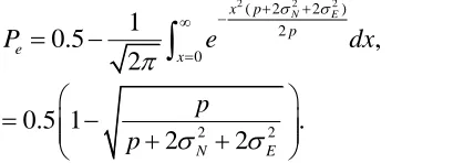
The average probability of error of the system is

2

2 0

1

,

2

x r e

r x p

P

e

dx e

dr







  _

 







(10)

where

2

2 2 2 2

(

_{N E}

)

_{N E}

r

r







 







(11)

Equation (10) can be simplified further to get

2

2

0 0

1

,

2

x k

r e

x r

P

e dre

dx





 _

 



 

(12)

where

2 2 2 2 2 2 4 2 2 2

(

)

(

)

4

.

2

N E

x

N E

x

px

N E

k

p

















 



On further simplification,

( ) 0

1

0.5

.

2

f x

e _x

P

e

dx



 _







_

(13)

where

2₍ 2 2_{) (} 2 2₎2 4 ₄ 2 2 2 ( )

2

N E N E N E

x p x px

f x

p

     

    



(14)

The integral in (13) cannot be directly evaluated and it is not even one of the standard integrals. We present two methods of evaluating the integral.

Method-1: Approximating 2 2 2 4 2 2 2 (NE) x 4px N E , in

f(x) as 2 2 2 (NE)x

2 2 2

(

2

2

)

( )

.

2

N E

x

p

f x

p









International Journal of Emerging Technology and Advanced Engineering

Website: www.ijetae.com (ISSN 2250-2459, ISO 9001:2008 Certified Journal, Volume 9, Issue 8, August 2019)

83

With this approximation the average probability of error becomes

2_{( 2} 2 ₂ 2₎

2 0

1

0.5

,

2

N E

x p p

e _x

P

e

dx

 



  











2 2

0.5 1

.

2

_N

2

_E

p

p











_

_



_

_









(16)

This is the closed form expression for the BER of the system which is the very close approximation of the actual BER and the corresponding plot is given in the results section.

Method-2: It can be evaluated is using numerical integration. To use numerical integration, we need to know until which finite value of x we should evaluate the integral so that the error in evaluating the integral is minimum. For a Gaussian function of variance



2 the value of the function becomes approximately equal to zero beyond

| | 4

x





, it is substantiated by

2

4

0

2

(4)

x

1,

x

erf

e

dx



 







(17)

which implies

2

4

0

x

x

e

dx

 _







(18)

Defining g(x) as the function obtained by dropping

x

2 term in the square root term of f(x), given by

2 2 2

(

2

2

)

( )

2

N E

x

p

g x

p











(19)

( )

g x

e

 is always greater than

e

f x( ) and it can be shown that

2 2

( ) 4

2 2

0.

N E

g x p

x p

e

dx

 

 _

  





(20)

so it is enough to integrate

e

g x( ) and hence

e

f x( ) till

2 2

4

2

_N

2

_E

p

p









. The plot of

e

f x( ) given in Fig. 1

[image:4.612.49.263.168.242.2]

supports this statement. For example with

Fig 1.The plot of

e

f x( ) Noise variance of -18dB and estimation error variances of -30 dB, 0 dB, and 20 dB

2

0.015

N





(-18dB) and



_E2



1

(0dB) the plot is becoming negligible after

4 2

2 (2 (0.015 1))

x



 



=2.8178.

This enables us to evaluate this integral using the numerical integration. In this work we use Simpson's rule for numerically evaluating the integral in (13). The simulation results of this numerical evaluation is shown in the later section.

We now consider two special cases where the integral in (13) has closed form representations.

Case I: In the absence of estimation error, with only the noise term, (13) reduces to

2_{( 2} 2₎

2 0

1

0.5

,

2

N

x p p e

x

P

e

dx





  









2

0.5 1

.

2

_N

p

p









_

_



_

_







(21)

This is the BER of the OFDM system with perfect channel estimation. This is therefore the lower bound on the achievable BER of the OFDM system with error in channel estimation.

Case II: If there is only estimation error, with no noise in the system, the probability of error becomes

2

0.5 1

.

2

e

E

p

P

p









_

_



_

_



International Journal of Emerging Technology and Advanced Engineering

Website: www.ijetae.com (ISSN 2250-2459, ISO 9001:2008 Certified Journal, Volume 9, Issue 8, August 2019)

84

16 QAM

For 16-QAM the probability of bit error for each channel realization is given by [11]

 

3

1

9

1

5

.

4

5

2

5

4

e

P



Q

_







_







Q





_







_



Q











(23)

In this case let us define

f x

₁

( )

,

f x

₂

( )

and

f x

₃

( )

as

( )

f x

given in (14) with the values of p as 0.2, 1.8 and 5 respectively. The integrals

1( )

1

0

1

,

2

f x

x

I

e

dx



 _







2( )

2 ₀

1

,

2

f x

x

I

e

dx



 _





_

3( )

3

0

1

2

f x

x

I

e

dx



 _







(24)

are either evaluated by approximating

f x

i

( )

similar to that given in (15) or by using Simpson's rule and the probability of bit error is calculated using the expression

1 2 3

3

1

1

(0.5

)

(0.5

)

(0.5

)

4

2

4

e

P





I





I





I

(25)

B. Effect Of Error Phase

In this section we discuss the effect of difference in the phase of the channel estimate only assuming that the phase is distributed uniformly in different ranges. With H(K) as the perfect channel frequency response, let the imperfect channel estimate be

H K

ˆ ( )



H K e

( )

j, where



is uniformly distributed in the range

  



_e

 

_e. The output of the matched filter in this case is

*

( )

( )

( ),

1,

,

.

p

R K



Y K H K

K

 

N

(26)

The probability of error for each realization for BPSK is 2

( 2

cos

)

Q

SNR



, and the average BER for any



is given by

2

2 2

cos

( )

0.5 1

,

cos

e

N

P





 









_





_







(27)

Averaging it over all possible values of



we get the average probability of error,

1

( )

2

e

e

e e

e

P



P

d















(28)

We get the average probability of error as

2 2

1

2

cos ( )

1

0.5

cos

2

1

N e

e N

P

























_



_







(29)

IV. RESULTS AND DISCUSSIONS

This section presents the BER performance of the OFDM system in the presence of channel estimation error. Particularly, we show that the calculated BER of (13) match closely the BER obtained using the monte-carlo simulations. We consider an OFDM system with perfect time and frequency synchronization

in all the performance results.

The BER of the OFDM system with error in channel estimation, in Rayleigh fading channel is calculated by evaluating (13). The integrand in (13) is shown in Fig.1 as a function of

x

, for the noise variance of 0 dB and the variances of the estimation error -30 db, 0 dB, and 20 dB. It can be seen that, the width of the integrand is maximum for the case of least estimation error (-30 dB) and the width is very small for the case of maximum estimation error (20 dB). Further, even the maximum width is very less since the integrand is becoming negligible before $x=4$. As the variance of the estimation error increases, the width of the function is decreasing to account for the increased probability of error. Considering this, we used the Simpson's rule with $x$ varying from zero and 10 in steps of 0.01.

Fig 2. gives the comparison of the calculated and simulated BERs for an OFDM system with

N



64

,

3

[image:5.612.47.161.282.376.2]

International Journal of Emerging Technology and Advanced Engineering

Website: www.ijetae.com (ISSN 2250-2459, ISO 9001:2008 Certified Journal, Volume 9, Issue 8, August 2019)

[image:6.612.51.287.146.313.2]

85

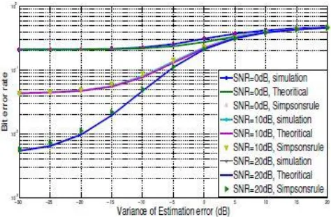
Fig 2. BER performance as a function of variance of channel estimation error for an OFDM system in Rayleigh fading channel, with N=64, L=3, and BPSK modulation, for SNR values of 0 dB, 10

dB, and 20 dB. Simulation and analysis

Fig 3. gives the comparison of the BERs calculated using Numerical integration of (13), the approximate form given in (16) and simulated BERs for an OFDM system with

N



64

,

L



3

, and QPSK modulation, as a function of the variance of the estimation error for different values of SNR. It can be observed that, the computed BER values based on the Gaussian approximation of the product of Gaussians match the simulated BER very closely.

Fig 3. BER performance as a function of variance of channel estimation error for an OFDM system in Rayleigh fading channel, with N=64,L=3 and QPSK modulation, for SNR values of 0 dB, 10

[image:6.612.325.562.180.349.2]

dB, and 20 dB. Simulation and analysis

Fig 4 gives the similar plot for 16-QAM modulation, as expected the probability of error is more than that of QPSK but varies in the same way.

Further, it can be seen that, the system performance degrades considerably when the variance of the estimation error becomes equal to the noise variance.

Fig 4.BER performance as a function of variance of channel estimation error for an OFDM system in Rayleigh fading channel, with N=64,L=3 and 16-QAM modulation, for SNR values of 0 dB, 10

dB, and 20 dB. Simulation and analysis

Fig 5 gives the comparison between the simulated performance of the system with only the phase error in the channel estimate uniformly distributed in the ranges

0.6



0.6



 

,



1.2

 



1.2

and



1.8

 



1.8

all in radians. For each case the calculated BER using the equation (29) is plotted. The plots show that the equation derived gives the exact degradation in the performance of the system.

Fig 5. BER performance as a function of phase error in channel estimate for an OFDM system in Rayleigh fading channel, with N=64,L=3 and BPSK modulation, for SNR values of 0 dB, 10 dB, and

[image:6.612.50.287.467.622.2] [image:6.612.329.562.503.667.2]

International Journal of Emerging Technology and Advanced Engineering

Website: www.ijetae.com (ISSN 2250-2459, ISO 9001:2008 Certified Journal, Volume 9, Issue 8, August 2019)

86

V. CONCLUSIONS

We derived expressions for the BER of the OFDM system with channel estimation error, based on Gaussian approximation of the product of Gaussians. The approximation is validated by showing that the calculated BER based on the Gaussian approximation matches closely the simulated BER values. The main conclusion drawn is that, an estimation procedure is optimum if the estimation error is considerably less than the noise variance.

REFERENCES

[1] J.A.C Bingham, ―Multicarrier modulation for data transmission: An idea whose time has come,‖ IEEE Comm. Mag., vol. 28, pp. 4-14, May 1990.

[2] Y.(Geoffery)Li and G.L.Stuber, ―Orthogonal frequency multiplexing for wireless communications, ―Springer, 2006.

[3] A.R.S.Bahal and B.R.Saltzberg ``Multi-Carrier Digital Communications:Theory and Applications of OFDM,'' Kluwer Academic/Plennum,1999.

[4] S. Coleri, M.Ergen, A.Puri and A.Bahai ―Channel Estimation Techniques based on Pilot arrangement in OFDM systems,‖ '' {IEEE Trans. Broadcast.,}vol. 48, no. 3, pp. 223-229, 2002.

[5] Y. Li, ―Pilot-symbol-aided channel estimation for OFDM in wireless systems,'' {IEEE Trans. Veh. Technol.,} vol. 49, no. 4, pp. 1207-1215, 2000.

[6] Y.Li, L. J. Cimini, and N. R. Sollenberger, ―Robust channel estimation for OFDM systems with rapid dispersive fading channels,‖ {IEEE Trans. Commun.,} vol. 46, no. 7, pp. 902-915, 1998.

[7] M.-H. Ng and S.-W. Cheung,― Bandwidth-efficient pilot-symbol-aidedtechnique for multipath-fading channels,'' { IEEE Trans. Veh. Technol.,} vol. 50, no. 4, 2001.

[8] J. K. Cavers,‖An analysis of pilot symbol assisted modulation for Rayleigh fading channels,'' {IEEE Trans. Veh. Technol.,} vol. 40, pp. 686-693, No. 1991.

[9] O. Edfors, M. Sandell, J.-J. van de Beek, S. K. Wilson, and P. 0. Bojesson,‖Ofdm channel estimation by single value decomposition,‖{IEEE Trans. On Comm.,}vol. 46, pp. 931-939, July 1998.

[10] H. Tang, K. Y. Lau, and R. W. Brodersen,‖Interpolation-Based Maximum Likelihood Channel Estimation Using OFDM Pilot Symbols,'' {Proc. IEEE Globecom Conf.,} vol. 2, Taipei, Taiwan, Nov. 2002, pp. 1860–64.

[11] Lie-Liang Yang and L.Hanzo,‖A recursive algorithm for the error probability evaluation of M-QAM'', IEEE Commun Letters, vol.4, no.10, pp.304-306,October 2000.

[12] J. G. Proakis, {\em Digital communications,} McGraw-Hill, New York, 2008.Fourth Edition pp. 43,46 equation 2.1-120,141. [13] I. S. Gradshteyn and Ryzihk,{Tables of integrals series and