Modal Characterization and Structural Dynamic Response of a Crane Fly Forewing

(1)

University of New Orleans University of New Orleans

ScholarWorks@UNO

University of New Orleans Theses and

Dissertations Dissertations and Theses

Fall 12-18-2014

Modal Characterization and Structural Dynamic Response of a

Crane Fly Forewing

Jose E. Rubio

University of New Orleans, [email protected]

Follow this and additional works at: https://scholarworks.uno.edu/td

Part of the Applied Mechanics Commons, and the Structures and Materials Commons

Recommended Citation Recommended Citation

Rubio, Jose E., "Modal Characterization and Structural Dynamic Response of a Crane Fly Forewing" (2014). University of New Orleans Theses and Dissertations. 1941.

https://scholarworks.uno.edu/td/1941

This Thesis is protected by copyright and/or related rights. It has been brought to you by ScholarWorks@UNO with permission from the rights-holder(s). You are free to use this Thesis in any way that is permitted by the copyright and related rights legislation that applies to your use. For other uses you need to obtain permission from the rights-holder(s) directly, unless additional rights are indicated by a Creative Commons license in the record and/or on the work itself.

(2)

Modal Characterization and Structural Dynamic Response of a Crane

Fly Forewing

A Thesis

Submitted to the Graduate Faculty of the University of New Orleans in partial fulfillment of the requirements for the degree of

Master of Science in

Engineering-Mechanical Solid Mechanics

by

José Enrique Rubio

B.Sc., University of New Orleans, 2012

(3)

ii

(4)

iii

(5)

iv

Acknowledgement

I would like to thank my major professor Dr. U. Chakravarty for giving me the

opportunity to be part of his research team. Such opportunity has definitely helped me to gain

on-hands research experience and to enhance my ability to work independently and think

critically. Most importantly, without Dr. Chakravarty’s knowledge, motivation, and mentorship

finishing this study would not have been possible.

I am extremely grateful to Dr. P. Schilling for being my undergraduate advisor and

serving as a committee member for my master’s thesis. His constant advices since the beginning

of my undergraduate career and his valuable input towards the completion of this research have

been a keystone for my personal and professional development throughout these years.

I would also like to extend my thanks to Dr. M. Guillot for serving as a committee

member for my thesis. His recommendations and support were fundamental to improve the

quality of this manuscript.

I would like to express my gratitude to my colleagues Manohar Chidurala and Pratik

Sarker for their constant help in building the computational models. Also, I extend my thanks to

William Miller for his assistance on the scanning of the specimen and to Claude Zeringue for his

help in the construction of the experimental setup.

Lastly, I feel indebted to my family for their endless support and encouragement. Thanks

(6)

v

Nomenclature

A – Surface area

D

C _{– Coefficient of drag}

L

C – Coefficient of lift

c – Chord length

D – Total derivative E – Modulus of elasticity

D

F _{– Drag force}

L

F – Lift force

g _{– Gravity or buoyancy force}

h – Thickness of shell

L – Characteristic length l – Length of flat plate

n – Normal direction to a referenced surface p _{– Pressure}

q _{– Distributed load}

Re – Reynolds number

V

S – Von-Mises stress

s – Span length

t – time

U – Deformation magnitude

x

U _{– Deformation component in}x-direction

y

U _{– Deformation component in}y-direction

z

U _{– Deformation component in}z-direction

V – Velocity

V_ – Freestream velocity

V – Velocity vector

x

(9)

viii y

v – Velocity component in y-direction

z

v – Velocity component in z-direction

w – Out of plane or transverse deflection x – Cartesian coordinate

y _{– Cartesian coordinate}

z – Cartesian coordinate

Greek symbols

 – Boundary layer thickness  – Angle of attack

ij

 – Kronecker’s delta function  – Dynamic or absolute viscosity  – Density

ij

 – Stress tensor

 – Poisson’s ratio  – Kinematic viscosity

 – Shell domain for vibration mathematical model  – Frequency

Symbols

 – Gradient vector

4

 – Biharmonic operator

 – Partial derivative or differential element _{– Clamped edge of shell}



(10)

ix

List of Figures

Figure 1.1. Boundary layer representation ...2

Figure 1.2. Insect wing terminology ...4

Figure 1.3. Flapping cycle of insects [3]...4

Figure 1.4. Clap mechanism (top) and fling mechanism (bottom) [3] ...6

Figure 1.5. Delayed stall and wake capture mechanism ...7

Figure 2.1. Typical adult crane fly (left) and metric scale for an adult crane fly (right) ...14

Figure 2.2. Crane fly forewing sample ...15

Figure 2.3. Typical micro-CT scan setup...17

Figure 2.4. Typical internal morphology of an insect wing [34] ...20

Figure 2.5. Reconstructed model of the crane fly forewing from the micro-CT scan at two different attenuation levels ...21

Figure 2.6. 2-D cross-sectional image for the identification of the veins ...22

Figure 2.7. Sliced cross-section from the reconstructed 3-D model ...22

Figure 2.8. Membrane part (left) and membrane mesh (right) ...24

Figure 2.9. Vein pattern part (left) and vein mesh (right) ...25

Figure 2.10. CFD domain (left) and CFD mesh (right) ...27

Figure 2.11. Mesh refinement near wing cavity ...27

Figure 2.12. Co-simulation interfaces for the FE model (left) and the for CFD model (right) ...30

Figure 3.1. Domain for the mathematical formulation of the modal analysis of the crane fly forewing ...32

Figure 3.2. Schematic for mathematical formulation of steady flow over an immersed body ...34

Figure 3.3. Schematic for mathematical formulation of unsteady flow over an immersed body ..38

(11)

x

Figure 4.2. First (at 79.97 Hz), second (at 347.89 Hz), third (at 442.52 Hz), and fourth mode shape (at 1042.9 Hz) of the crane fly forewing in vacuum ...44

Figure 4.3. Comparison between the CFD model solution and the Blasius solution for Vx velocity

profile along the trailing edge of the flat plate ...46

Figure 4.4. Location of node A and central path along spanwise y-direction for monitoring of convergence and analysis of results, respectively ...47

Figure 4.5. Mesh independence study for the FSI simulation done by monitoring the variation of the deformation of node A with respect to a change of the number of nodes in the FE mesh only ...47

Figure 4.6. Mesh independence study for the FSI simulation done by monitoring the variation of the total lift force on the FSI surface with respect to a change of the number of nodes in the CFD mesh only ...48

Figure 4.7. Deformation (left) and Von-Mises stress (right) of the crane fly forewing under steady airflow at 10 mm/s (first row), 50 mm/s (second row), 100 mm/s (third row), and 1000 mm/s (fourth row) ...50

Figure 4.8. Deformation magnitude along a central path in the spanwise y-direction for steady airflow at different freestream velocities ...51

Figure 4.9. Aerodynamic efficiency of the crane fly forewing at different freestream velocities .51

Figure 4.10. Deformation magnitude along a central path in the spanwise y-direction for steady airflow at a freestream velocity of 1000 mm/s ...52

Figure 4.11. Ux (left), Uy (center), and Uz (right) components of displacement for steady airflow

at a freestream velocity of 1000 mm/s ...53

(12)

xi

List of Tables

Table 1.1. MAVs design requirements as outlined by the Defense Advanced Research Projects

Agency (DARPA) [4, 5] ...8

Table 2.1. Morphological and kinematic parameters for the crane fly [23, 24] ...15

Table 2.2. Micro-CT scanning setup setting ...19

Table 2.3. Final dimensions of the reconstructed model ...21

Table 2.4. Geometric parameters of the FE model ...23

Table 2.5. Material properties for the FE model ...26

Table 2.6. Fluid properties for the CFD model ...28

Table 2.7. Boundary conditions for the CFD model ...29

Table 4.1. Comparison between the natural frequencies of the FE elliptical model and the analytical solution in vacuum ...41

Table 4.2. Natural frequencies of the crane fly forewing in vacuum ...43

(13)

xii

Abstract

This study describes a method for conducting the structural dynamic analysis of a crane

fly (family Tipulidae) forewing under different airflow conditions. Wing geometry is captured

via micro-computed tomography scanning. A finite element model of the forewing is developed

from the reconstructed model of the scan. The finite element model is validated by comparing

the natural frequencies of an elliptical membrane with similar dimensions of the crane fly

forewing to its analytical solution. Furthermore, a simulation of the fluid-structure interaction of

the forewing under different airflows is performed by coupling the finite element model of the

wing with a computation fluid dynamics model. From the finite element model, the mode shapes

and natural frequencies are investigated; similarly, from the fluid-structure interaction, the

time-varying out-of-plane deformation, and the coefficients of drag and lift are determined.

Keywords: Fluid structure interaction, finite element model, crane fly, structural response,

(14)

1

CHAPTER 1. INTRODUCTION

Insects are by far the oldest, most numerous, and smallest flying organisms which have

had an important evolutionary success due to their superlative maneuverability during low-speed

flight. Flying insects, in general, experience highly elastic deformations in their wings during the

flapping cycle to create the aerodynamic forces that allow them to hover and to maneuver. The

study of flapping flight has captivated and motivated scientists to perform quantitative and

qualitative descriptions of the kinematics and the mechanical and aerodynamic principles that

govern insect flight. The significance of such detailed studies is the potential application of these

aerodynamic principles into engineered devices, e.g. biologically inspired micro air vehicles

(MAVs). Moreover, in order to successfully biomimic the aerodynamic performance of insects,

the MAVs must have a robust design with efficient, optimized wing structures such as those

from insects. This study concentrates on characterizing the structural dynamic response of the

crane fly, an insect, in vacuum and under different airflow conditions. Specifically, the

deformation and aerodynamic performance of the crane fly forewing are investigated.

1.1. Flow over Immersed Bodies

External flow past an object involves different fluid mechanics phenomena. For a given

shaped object, the characteristics of the flow depend strongly on various parameters such as the

size and orientation of the object, the speed of the fluid, and the fluid properties. Furthermore,

the character of the flow is governed by different dimensionless parameters. For typical external

flow, the most important parameter is the Reynolds number which is defined as the ratio of the

inertial forces to the viscous forces and mathematically expressed in Eq.1.1. [1]

Re V L



(15)

2

In general, if the Reynolds number is small, the inertia effects are relatively small

compared to the viscous effects. Moreover, if the Reynolds number is large, the region in which

the viscous effects are dominant is allocated very close to the surface of the immersed body

while the rest of the flow field is dominated by inertial effects. The region in which the viscous

effects dominate is known as the boundary layer and its thickness increases in the direction of

flow. Furthermore, within the boundary layer, the velocity changes from the freestream velocity

to zero velocity on the surface of the immersed body. The reason for the existence of this

boundary layer is that the viscosity of the fluid is not zero; consequently, the fluid must stick to

the solid surface, this is known as the no-slip boundary condition. This thin boundary (thin

compared to the length of the object) is responsible for the production of the lift and the drag

forces and it is approximately represented in Fig 1.1.

Figure 1.1. Boundary layer representation

When a fluid moves over an immersed body, an interaction occurs which can be

described in terms of the forces at the fluid-body interface. The resultant force in the direction of

the flow is called drag; while the resultant force in the normal direction to the flow is termed lift.

Referring to Fig.1.1, the lift and the drag forces are mathematically defined in Eqs. 1.2 and 1.3,

respectively [1].

D x

F 



p dA (1.2)

L n

(16)

3

The generation of these two forces is directly related with the pressure distribution along

the surface area of the immersed body. In general, when a fluid flows past a non-symmetric

object, the pressure field is not uniform. As discussed previously, a relatively thin boundary layer

is developed along each of the surfaces of the immersed body; within this layer, the component

of the pressure gradient in the direction of the flow is not zero, while the component in the

normal direction is negligibly small. This pressure gradient is caused by the variation of the

freestream velocity across the boundary layer and it generates the so-called drag and lift forces.

Alternatively, the drag and lift forces can be defined in terms of dimensionless parameters called

the drag and lift coefficients which are defined in Eqs. 1.4 and 1.5, respectively [1].

2

1 2

D D

F C

V A  _

 (1.4)

2

1 2

L L

F C

V A  _

 (1.5)

1.2. Insect Flight Kinematics

An understanding of basic wing terminology is required before proceeding with any

further discussion. The morphology of a typical insect wing, presented in Fig. 1.2, has two main

features: the leading edge and the trailing edge, which refer to the foremost and rear edge of the

wing, respectively. Furthermore, the wing span is referred as the distance from the tip of the

wing to the root of the wing where it intersects with the thorax of the insect. On the other hand,

the chord length is defined as the distance between the trailing edge and the corresponding point

(17)

4

Figure 1.2. Insect wing terminology

The flapping cycle of an insect is conformed of two translational phases: downstroke and

upstroke; and two rotational stages: pronation and supination, all of them depicted in Fig. 1.3.

Downstroke and upstroke occur when the wing translates over the air at a higher angle of attack.

Moreover, wing pronation occurs during the transition from upstroke to downstroke and it

consists in the inward rolling of the wing towards the thorax of the insect; on the other hand,

supination occurs during the transition from downstroke to upstroke and it consists in the

outward rolling of the wing towards the torso of the insect [2, 3].

Figure 1.3. Flapping cycle of insects [3]

Identifying the manner in which insect wings provide the needed lift for flight has been

extremely difficult. Their small scale and rapid wing-beat make experimental measurements

problematic and collecting data from tethered insects may often yield data based on unnatural Chord

Span Leading Edge

(18)

5

movements. However, some principles have been identified using mechanical models that are

matched to that of an actual insect, ensuring that the governing fluid dynamic phenomena are

conserved. These models together with advanced experimental setups such as high-speed

cameras, digital image correlation software, and particle image velocimetry systems have made

possible the identification and analysis of the different unsteady mechanisms that govern the

kinematics of insect flight.

It is essential to remark that insects do not create the required lift forces by simply

flapping their wings since the effects of the downstroke would be aerodynamically cancelled out

by the equivalent ones from the upstroke [4]. Instead, insects generate the needed lift and thrust

by experiencing unsteady aerodynamic mechanisms coupled with highly elastic deformations in

their wings derived from the aerodynamic loading from flapping flight. Three unsteady

mechanisms have been identified in the aerodynamics of insect flight, although the occurrence of

all the three of them is not guaranteed in every insect. The first mechanism, the clap and fling

mechanism shown in Fig.1.4, consists of raising the wings so the tips touch dorsally before they

pronate. The leading edges touch each other or “clap” before the trailing edges, progressively

closing the gap between them and forming a shape similar to a vertical plate. As the wing presses

together closely, the opposing circulations of each of the wings are canceled out each other. The

wings are then quickly pronated with the leading edges “fling” apart, creating a low-pressure

region between them that causes the gap to be filled with entering air, consequently providing an

initial momentum and a vortex of air [3, 4]. Collectively, the clap and fling mechanism results in

a modest, but significant, lift enhancement. The second well-identified unsteady mechanism in

insect flight is the delayed stall and it is shown in Fig. 1.5. As the wing increases its angle of

(19)

6

before it reaches the trailing edge. In such cases, a leading edge vortex occupies the separation

zone above the wing. If the wing translates at a higher angle of attack, the leading edge vortex

grows in size until flow reattachment is no longer possible. As a result, there is a drop in the lift

and the wing is said to have stalled. For several chord lengths prior to the stall, the presence of

the attached leading edge vortex produces very high lift coefficients, a phenomenon termed

“delayed stall” [3, 4] . Delayed stall has been highly associated with the deformation experienced

by insects at low Reynolds number. The third unsteady mechanism is the wake capture and

rotational circulation. The former allows the wing to take advantage of the wake created by the

previous stroke while the latter allows an upward lift to be generated when the wing’s own

rotation creates air circulation at the end of the stroke [3, 4].

(20)

7

Figure 1.5. Delayed stall and wake capture mechanism [3]

1.3. Micro Air Vehicles

Understanding the role of wing flexibility in producing unsteady aerodynamic forces and

mechanisms that enable flapping flight is fundamental for the potential emulation of flapping

flight in man-made manufactured devices. Moreover, characterizing the structural response of

insect wings to dynamic loading is seen as the keystone for the development of the new

generation of high-performance and aerodynamically efficient MAVs.

MAVs are autonomous, lightweight, small-scale flying devices with a maximum wing

span of 15 cm and a maximum flying speed of approximately 15 m/s as detailed in Table 1.1.

Interest in the design of these aerial devices has immensely grown over the last years due to their

potential to operate in remote or otherwise hazardous locations where they may perform a variety

of tasks, including but not limited to, reconnaissance, surveillance, and safety inspection. To

accomplish the aforementioned tasks, the wings of MAVs should be aerodynamically efficient,

optimized structures; such as the wings found in different insects. Currently, extensive research

is being done to design biologically inspired MAVs that mimic the superlative maneuverability

(21)

8

Table 1.1.MAVs design requirements as outlined by the Defense Advanced Research Projects Agency (DARPA) [5, 6]

Specifications Requirements Details

Size <15.24 cm Maximum dimension

Weight ~100 g Objective gross takeoff weight (GTOW) Range 1 to 10 km Operational range

Endurance 60 min Loiter time on station Altitude <150 m Operational ceiling

Speed 15 m/s Maximum flight speed

Payload 20 g Mission dependent

Cost $1500 Maximum cost, 2009 USD

1.4. Literature Survey

Detailed research on the field of aerodynamics of insects traces back from about 40 years

ago. A pioneer work on this field was presented by Ellington through his compendium of studies

about the aerodynamics of hovering insect flight [7‒12]. Ellington re-examined and questioned

the conventional quasi-steady assumption proposed by Weis-Fogh [13, 14], which assumed that

the instantaneous forces on a flapping wing were equivalent to those for steady motion and

concluded that the aforementioned theory lacked of high fidelity evidence. First, Ellington

analyzed the principles and the validity of the quasi-steady assumption to conclude that further

studies were required to confirm such theory [7]. Consequently, he investigated and presented a

list of morphological and kinematic data for a variety of insects [8, 9]; which he then used to

offer an aerodynamic interpretation of the kinematics of insect wings and a discussion on the

possible roles of different aerodynamic mechanisms [10]. From the previous study, it was

determined that leading edge separation bubbles were prominent features in insect flight causing

flow to separate at the leading edge and then to reattach downstream to the upper wing surface;

consequently, producing a region of recirculating flow which improved the lift at low Reynolds

(22)

9

the lift and power requirements of hovering flight and a development of a vortex theory for lift

generation in insects [11, 12].

The previously described studies provided a novel insight about the aerodynamics of

insect wings and led to the development of research that concentrated on characterizing the

functional morphology of insect wings, outlining the principles of the biomechanics of insect

flight, and describing on detail the load bearing capacity of insect wings [15‒18]. Ennos and

Wootton [15] and Wotton [16, 17] experimentally investigated various features of different

insect species including their morphology, flight mechanics, and control behavior. Their work

suggested that the wings cambered and twisted slightly due to inertial forces. Furthermore, they

determined that both bending and deformation were highly dependent on the structure and

venation morphology of the wing and that these altered the direction and magnitude of

aerodynamic force production. Specifically, the bending and the deformation enhanced thrust

production by creating an asymmetric force between half-strokes and increased lift production by

allowing wings to twist and to generate upward force throughout the stroke cycle. Quite similar

findings were reported by Yin and Luo [18] who simulated the fluid-structure interaction (FSI) in

hovering flight to investigate the effect of inertia and fluid deformation on hovering

performance. They reported that both inertia-induced and flow-induced deformation could

enhance the lift generation of the wing.

Wing flexibility plays an important role when characterizing the deformation experienced

by insects during aerodynamic loading; therefore, different experimental studies have directed

their objectives towards finding the relationship that best describes the dependence of wing

deformation with respect to wing flexibility. Combes and Daniel [19, 20] addressed the

(23)

10

wings due to an applied point load and quantifying wing venation variation in different insect

species. They concluded that flexural stiffness declined sharply from wing base to tip and from

the leading to the trailing edge. Ishihara et al. [21] studied the two-dimensional (2-D) FSI in

Dipterian flapping flight; specifically, they concentrated on the passive pitching due to wing

torsional flexibility. It was demonstrated that insects kept the high angle of attack during its

translation and that the pitch angle rotated at the stroke reversal. Furthermore, they concluded

that it is especially important that the wing begins to twist before it changed its flapping direction

so that it could generate the required lift.

Several studies have used numerical methods, such the finite element (FE) method, to

simulate wing structures and compare their results with experimental data. Combes and Daniel

[22] addressed the relative contributions of aerodynamic and inertial-elastic forces to wing

bending in a Manduca sexta forewing by using experimental data and a FE model. Their results

suggested that a damped FE model, with realistic forces applied at the base, could be successful

in predicting the overall pattern and the magnitude of the insect wing deformation during flight,

independently of aerodynamic calculations. Sims et al. [23] conducted an experimental structural

analysis of a dragonfly, Manduca sexta, forewing by collecting frequency data using laser

vibrometry in air and in vacuum and comparing the results with a computational model. They

concluded that camber was an important structural property for the Manduca sexta. Jongerius

and Lentink [24] conducted a similar structural analysis directed to determine how the wings of a

dragonfly, Sympetrum vulgatu, carried the aerodynamic and inertial loads during regular insect

flight using an approximated mathematical inertial load model. Rubio et al. [25] investigated the

structural response of a symmetric sail-like insect wing model inspired from a crane fly

(24)

11

The progress on the characterization of insect flight has foster a new multi-disciplinary

collaboration, between biologists who seek to understand how the aerodynamic loads are related

to insect physiology and evolution, and engineers who aspire to build micro-robotic insects using

these principles. This trend has led to different investigations concentrating on the biomimetic of

insect flight characteristics in MAVs. Ellington [26] studied the aerodynamic characteristics of

insects applicable to MAVs. He presented different design characteristics of insect-based flying

devices and estimates of the mass they could support, their mechanical power requirement, and

their maximum flight speeds over a wide range of sizes and frequencies. His work suggested that

for the simplest implementation of insect features into MAVs a simple sail-like construction

would suffice with features such as a stiff leading edge supporting a membrane and independent

adjustment of both the flapping amplitude and the mean flapping angle.

Further research efforts have been done in smart materials that could potentially

biomimic the structural characteristics of insect wings. Chakravarty [27] investigated the

vibration characteristics of biologically inspired wings fabricated from composite polyester

materials. He concentrated on investigating the effect of added mass, aerodynamic pressure, and

damping on the vibration characteristics of such wings. An inversely proportional relationship

was found between the magnitude of the natural frequency and the added mass. Moreover,

Chakravarty and Albertani [28] investigated the effects of aerodynamic loads on the modal

characteristics on a biologically inspired wing fabricated from a hyperleastic membrane. They

determined that the natural frequency of a membrane increased with pre-strain level and that the

damping of air had minimal effect on the natural frequencies of the wing but assisted on reducing

the out-of-plane modal amplitude of vibration. Wu et al. [29] studied the structural properties of

(25)

12

pairs of hummingbird-shaped membrane wings of different properties at atmospheric pressure

and in vacuum. They described the aeroelastic behavior of the wings and visually explained the

relationship between flexibility and thrust production. Their research supported that wing

deformation was a vital feature for generating aerodynamic thrust in insects indicating the

important role of flexibility in bio-inspired wings.

1.5. Motivation and Objective of Study

The special attention drawn to biomimic insect wings which could potentially be

implemented into MAVs is the motivation for this study. In order to develop structures that could

demonstrate the same excellent structural response of insect wings, one must first be able to

thoroughly analyze the aerodynamic behavior of insect wing in vacuum and under airflow

conditions and then translate such behavior into the engineered structure. Few studies, to the

knowledge of the author, have been developed to analyze the FSI of insect wings to quantify the

structural dynamic response of the wings in terms of deformation and aerodynamic variables,

namely lift and drag forces. Therefore, this manuscript presents a numerical method for

investigating the structural dynamic response of a crane fly forewing, an insect in the family

Tipulidae. The aim of this study can be decomposed into two sections:

1) Characterization of the external and internal morphologies of the crane fly

forewing: The inherent scale of insects makes the accurate description of the structure of

the wing a cumbersome task. Furthermore, insect wings are characterized by complex

wing patterns that intersect at multiple times and that are hold together by a thin

membrane. Given this complexity, a wing sample is digitally captured using a

micro-computed tomography (micro-CT) scanner which is the most advanced three dimensional

(26)

13

model the external and internal morphologies of the wing are subsequently transferred

into a FE model.

2) Investigation of the structural dynamic response of the crane fly forewing:

Quantifying the instantaneous deformation on insect wings helps determine the direction

and magnitude of fluid-dynamic forces generated by the inertial and aerodynamic load;

therefore, being able to predict large, dynamic shape changes is essential for developing a

comprehensive understanding of insect flight. The FE model, developed from the

micro-CT scan, is used to perform a complete modal analysis of the forewing in vacuum.

Similarly, FSI simulations under steady and unsteady conditions at low freestream

velocities are performed by coupling the FE model of the forewing with a computational

fluid dynamics (CFD) model. The deformations and aerodynamic coefficients of the

(27)

14

CHAPTER 2. MATERIALS AND METHODS

2.1. Specimen Characterization

2.1.1.Selection and Description of the Specimen

A crane fly forewing is used for the development of this study. This insect belongs to the

family Tipulidae [30] which may be recognized by their slender bodies and long, slender legs.

Common nicknames for this specimen are “daddy-long-legs”, “golly whopper”, and “mosquito

hawk”. The selection basis is rather arbitrary within the framework of insect specimens that are

proven to be aerodynamically efficient at low-speed flight and hovering [8]. A picture of a

typical adult crane fly is presented in Fig. 2.1 (left) and a summary of morphological and

kinematic parameters, which are averaged from different specimens in references [23, 24], is

described in Table 2.1. It is noteworthy the size scale of the crane fly with a miniature wing span

in the order of 10-3 m. This scale can also be seen in Fig. 2.1 (right) which presents a dried

specimen of a crane fly next to a millimeter metric scale. Furthermore, it is noticeable the

flapping frequency of 45.5 Hz at low-speed flow regimens from the crane fly which is reasonable

as small insects tend to have higher flapping frequencies.

(28)

15

Table 2.1. Morphological and kinematic parameters for the crane fly [23, 24]

Parameter Value

Wing span length (per wing) 12.7 mm Averaged chord length 2.37 mm Wing pair area 59 mm2 Wing pair mass 0.000245 g Total insect mass 0.0114 g

Stroke angle 123°

Flapping frequency 45.5 Hz Reynolds number 20 < Re < 200

2.1.2.Specimen Evaluation

The crane fly forewing is a rather complex structure as it can be seen from Fig. 2.2. There

are several veins, many of which intersect multiple times, attached to a membrane. Moreover, a

meticulous visual inspection may reveal different vein thicknesses but surely their magnitudes

cannot be determined from this inspection. Prior proceeding with developing any FE model, a

high-fidelity structural characterization of the wing is required. Because of the small scale of the

specimen and the complexity of the wing structure, the number of instruments and techniques

capable of providing accurate quantitative description of the external and internal morphologies

of the crane fly forewing are limited. One solution to this intrinsic problem is to characterize the

structure of the wing using micro-CT scan, the most advanced non-intrusive 3-D microscopy

technique.

(29)

16

2.2. Micro-CT Scan

2.2.1.Background

To analyze the structural dynamic response of the crane fly forewing, a 3-D

characterization of the wing structure is required. Conventional optical microscopy allows

visualizing 2-D images of the specimen surface. However, in most of the cases, a conclusion

about the 3-D structure cannot be made on the basis of 2-D information. One alternative to

obtain 3-D information of the structure of the specimen is to cut the specimen into very thin

slices, then use an optical microscope to visualize and analyze the structure, and finally

interpolate the 2-D information into the 3-D model. However, this method is not only very

cumbersome but also unreliable since the structure of the specimen itself can be altered by the

intrusive preparation technique, especially with fragile structures such as insect wings. A more

accurate non-intrusive method is required to characterize the internal structure; therefore,

micro-CT scanning is selected as the most appropriate method to digitize the wing sample since it

provides a complete and precise representation of the 3-D structure of the wing.

2.2.2.3-D X-Ray Microscopy Principle

3-D X-ray microscopy allows reconstructing, visualizing, and measuring complete 3-D

structures without sample preparation. The principle behind computed tomography is the

interaction of ionizing radiation absorption between an X-ray source and a sample subjected to

the scan. A CT image is created by directing X-rays through the slice plane from multiple

orientations and measuring their resultant decrease in intensity. The simplest micro-CT scan

setup is shown in Fig. 2.3 and it consists of an X-ray source, a sample, and an X-ray detector that

measures the extent to which the X-ray signal has been attenuated by the sample. As the X-ray

(30)

17

the different materials that compose the sample along its path [31]. Furthermore, the actual

attenuation not only depends on the density of the sample material but also on the energy

spectrum from the X-ray source. To accurately produce a 3-D CT image, a whole set of 2-D

projections needs to be collected by a planar detector. Based on multiple angular views acquired

while the object rotates, a computer synthesizes a stack of virtual cross-section al slices through

the object to build a 3-D digital model [32].

Figure 2.3. Typical micro-CT scan setup

2.2.3.Stages of Micro-CT Scan

To reconstruct a 3-D digital model from a set of 2-D cross-sectional projected images, the

following stages are required during a micro-CT scan: acquisition, reconstruction, and

transformation from cross-section to image. The next paragraphs present a brief description of

the aforementioned stages, leaving algorithm and mathematical details out of the discussion

since they are out of the scope of this study.

1) Acquisition: During the acquisition stage, the sample rotates over 180° or 360° with a

fixed rotational step. At each angular position a shadow or projected image is acquired as

a 16 bit Tagged Image File Format (TIFF) file [32] by the 2-D detector.

2) Reconstruction: Using the Feldkamp reconstruction algorithm [33], also known as back

(31)

18

acquired cross-sectional projected images is generated. This raw data is not yet an image;

it is a floating point matrix holding the absorption values from the reconstructed

cross-sections.

3) Cross-section to image: This stage consists of generating the 3-D image from the

cross-section slices. The data from the floating point matrix is converted into a gray scale

image. The minimum and maximum attenuation are identified and the rest of the values

between this range are displayed as halftone. The reconstructed array is shown as a

half-tone image of the cross section with linear conversion to 256 grades of gray inside the

selected density interval.

2.2.4.Scanning Setup

For this study, a SkyScan 1172 high-resolution micro-CT scanner is used. A crane fly

forewing is collected and placed inside the scanner chamber using one of the sample holders. No

preparation is required on the sample; however, special care is taken to avoid damage or

alteration to the structure of the wing. Using the acquisition software from the scanner, the

acquisition settings are adjusted to achieve a good contrast between the different structures of the

wing, namely the membrane and the veins. This procedure is quite challenging given the size and

inherent transparency of the crane fly forewing, which makes the wing structure hard to

appreciate in the preview snapshots. Furthermore, the densities of the membrane and the veins do

not differ significantly; therefore, the scanning process is more difficult given that their X-ray

absorption rates are very similar.

In general, most of the acquisition settings are determined by trial and error; however,

few trends are noticed during this experimental stage. For this application, increasing the energy

(32)

19

contrasts in a specific material; thus, there is not sufficient differentiation, i.e. changes in

material density and composition, between features of interest. Furthermore, objects with a low

rate of X-ray absorption are scanned more effectively if no filter is present. Filters are commonly

flat or shaped pieces of metal such as copper, brass or aluminum, commonly used to absorb the

low energy beam of rays in the spectrum. Lastly, a small rotational step for a complete revolution

around the specimen is desired due to the asymmetric features of the insect wing. The complete

lists of acquisition settings used for the scanning process of the crane fly forewing are presented

in Table 2.2.

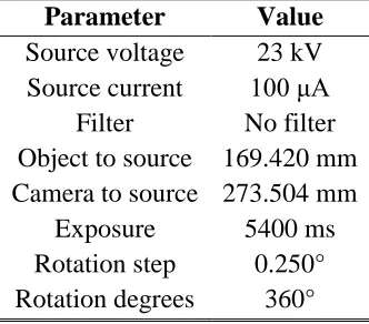
Table 2.2. Micro-CT scanning setup settings

Parameter Value Source voltage 23 kV Source current 100 μA

Filter No filter Object to source 169.420 mm Camera to source 273.504 mm

Exposure 5400 ms Rotation step 0.250° Rotation degrees 360°

2.2.5.Characterization of the External and Internal Morphologies of the Crane Fly Forewing

The structure of an insect wing is evolutionary determined by the need to optimize the

production of favorable aerodynamic forces during flight. Fully functional wings are found only

in adult insects and their external and internal morphologies are quite unique with some general

characteristics that are common for all species. Each of the wings of an insect consists of a thin

membrane supported by a number of well-marked veins running along the span- and chordwise

direction of the wing and connected to each other by cross-veins. In very small insects, the

(33)

20

through the branching of existing veins to produce accessory veins. The structure of an

individual vein reflects its role in the production of useful aerodynamic forces by the wing as a

whole. On the leading edge of the wing, the longitudinal veins form a rigid structure supporting

the wing as it moves through the air. On the other hand, at the tip of the wing the lack of veins

of significant diameter creates a flexible region. Furthermore, as shown in Fig. 2.4, the

membrane of an insect wing is formed by two layers of cuticle closely apposed; only separated at

the locations where the veins are formed. Moreover, the cuticle surrounding the veins becomes

thickened to provide strength and rigidity to the wing [34].

Figure 2.4. Typical internal morphology of an insect wing [34]

The geometry and structure of the crane fly forewing can be accurately described from

the reconstructed model of the micro-CT scan. The final parameters of this model are within

expected values when compared to the experimental ones presented in Table 2.3. Furthermore,

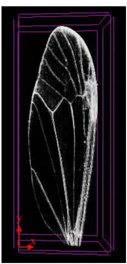
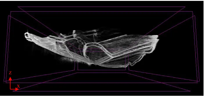
Fig. 2.5 presents a front view of the reconstructed forewing where the membranes and the veins

are clearly distinct with different attenuation gray scales. As expected, the venation pattern

presents a darker gray scale compared to the one from the membrane. Similarly, the thick veins

have a darker gray scale than the one from the thin veins which almost matches the

(34)

21

Table 2.3. Final dimensions of the reconstructed model

Parameter Reconstructed model value

Experimental value [18, 21]

Pixel size 5.3507 μm × 5.3507 μm --

Average chord length 3.007 mm 2.37 mm

Span length 13.86 mm 12.7 mm

Figure 2.5. Reconstructed model of the crane fly forewing from the micro-CT scan at two different attenuation levels

An interesting structure is observed during the analysis of the internal morphology of the

crane fly forewing. Figures 2.6 and 2.7 present images of the cross-section at approximately half

the span length of the wing. From these figures, two separated thin layers of cuticle are observed.

This gap between these two layers it to some extent inaccurate since insect wings are formed by

two layers of cuticle which are very close together, only separated at the locations where the

veins are formed, as presented in Fig. 2.4. Nevertheless, this phenomenon is explained by having x

y

(35)

22

used a dry specimen in which the two layers of cuticle are separated. Therefore, the total

thickness of the membrane is calculated by averaging the thicknesses of these two layers.

Furthermore, using the sliced cross-sectional images, the different diameters of the insect veins

with their respective wall thicknesses are accurately determined.

Figure 2.6. 2-D cross-sectional image for the identification of the veins

Figure 2.7. Sliced cross-section from the reconstructed 3-D model

2.3. Computational Model

2.3.1.Finite Element Model

2.3.1.1.FE Geometry Construction

The commercially available FE analysis package Abaqus 6.12 [35] is used to develop an

Abaqus/Standard FE model. The FE model is developed considering the curvature in z-direction

Veins

Cuticle

x z

Veins

(36)

23

to be much smaller than the spanwise y-direction, as seen on the scanned model. The FE model

is composed of two parts: membrane and veins.

To determine the dimensions of the contour of the wing, computational measurements of

the chord length of the wing are extracted along a central vertical axis for every 0.1605 mm (30

pixels) using the SkyScan CT Analyzer software V. 1.13.2.1 and the 2-D cross-sectional images.

The measurements are written into a data file which is then imported into Abaqus 6.12. The

dimensions of the FE model are approximately 3.007 mm in the chordwise x-direction and 13.86

mm in the spanwise y-direction, which fairly agrees with the dimensions of the reconstructed

model and with the measurements of the forewing of a crane fly reported by Ishihara et al. [21].

Membrane thickness is manually measured and assumed to be constant throughout the entire

wing. Furthermore, two sections of different vein thicknesses are identified through the scan

measurements and consequently developed in the FE model to take into account the variation of

the stiffness along the wing. The resolution of the scan allows for the identification of only two

diameters of veins thicknesses. Lastly, the veins are assigned a tubular profile as observed

through the computational measurements and confirmed by Agrawal et al. [36]. Table 2.4

presents a summary of the dimensional parameters of the FE Model.

Table 2.4. Geometric parameters of the FE model

Parameter Value

Span length 13.86 mm

Average chord length 3.01 mm Membrane thickness 0.016 mm Thick vein outer diameter 0.11 mm Thick vein wall thickness 0.04125 mm

(37)

24

2.3.1.2.FE Mesh Description

The membrane is modeled as a 3-D homogeneous shell with a constant thickness and it is

meshed using S4R (4-node general-purpose shell) type of element. These types of elements are

ideal to model structures in which one dimension, the out-of-plane thickness, is significantly

smaller than the other dimensions. Conventional shell elements use this condition to discretize a

body by defining the geometry at a reference surface. In this case the thickness is defined

through the section property definition. Furthermore, these types of elements have displacement

and rotational degrees of freedom. The membrane part and its respective mesh are shown in Fig.

2.8.

Figure 2.8. Membrane part (left) and membrane mesh (right)

On the other hand, the veins are modeled as 3-D wires with a tubular cross-sectional

profile. The veins are meshed using B32 (3-node quadratic beam) type of element. A beam

element is a one-dimensional line element in a 3-D space that has stiffness associated with

(38)

25

these elements have six degrees of freedom. The vein pattern and its respective mesh are shown

in Fig. 2.9.

Figure 2.9. Vein pattern part (left) and vein mesh (right)

2.3.1.3.Materials Properties for the FE Model

Material properties for a crane fly (family Tipulidae) are required for the FE model. The

material density of the wing cuticle is assigned to 1200 kg/m3 as measured by Wainwright et al.

[37] and used by Jongerius [24] and Ishihara [21]. A Poisson’s ratio of 0.495 is used as measured

in some biological materials by Wainwright et al. [37]. The effects of variation of Poisson’s

ratio can be considered negligible as investigated by Combes and Daniels [18]. Special care

must be taken when assigning the Young’s modulus. Recent studies reveal that the Young’s

modulus can vary widely within a wing as reported by Agrawal et al. [36], Combes and Daniels

[20], and Smith et al. [38]. Unfortunately, accurate data regarding the variation of Young’s

modulus along the wing span of insects is still limited. However, to take into account the

variation of stiffness along the spanwise y-direction of the wing, two sections of different vein

(39)

26

implemented into the FE model as done by Sims et al. [23]. For this FE model, the membrane

and the veins are assigned a Young’s modulus of 1.9 GPa and 4.0 GPa, respectively [23]. The

material properties for the FE model are summarized in Table 2.5.

Table 2.5. Material properties for the FE model

Property Membrane Veins Young’s modulus (GPa) 1.9 4.0

Poisson’s ratio 0.495 0.495 Density (kg/m3) 1200 1200

2.3.1.4.Boundary Conditions and Constraints for the FE Model

For accurate physical behavior, the FE wing model must mimic the physical in-flight

characteristics of a crane fly. Therefore, a clamped condition with all degrees of freedom fixed is

assigned to the base of the wing to simulate the corresponding condition of a wing attached to

the thorax of the insect. Similarly, a tie constraint is applied between the membrane and the veins

so that they act as a single deformable body with the deformations coupled between each other.

2.3.2.Computational Fluid Dynamics Model

2.3.2.1.CFD Geometry Construction

An Abaqus/CFD model is developed to represent the surrounding air flowing over the

wing. The CFD computational domain is modeled as a rectangular box that encloses a cavity

with the exact dimensions of the forewing. The size of the CFD domain is chosen to be 30 mm

height × 50 mm width × 70.0 mm length. With this dimensions the far-field boundaries are far

(40)

27

2.3.2.2.CFD Mesh Generation

The fluid domain is meshed using FC3D4 (4-node linear tetrahedral elements) type of

element. The mesh is refined near the wing cavity to reduce the aspect ratio between the mesh of

the CFD model and the mesh of the FE model. The respective fluid domain and its mesh are

shown in Fig. 2.10. Furthermore, the mesh refinement is presented in Fig. 2.11.

Figure 2.10. CFD domain (left) and CFD mesh (right)

Figure 2.11. Mesh refinement near wing cavity

2.3.2.3.Materials Properties for the CFD Model

Air properties at standard atmospheric conditions are assigned to the CFD model. The

(41)

28

Table 2.6. Fluid properties for the CFD model

Property Value

Air density (kg/m3) 1.225 Dynamic viscosity (kg/m∙s) 1.983×10-5

2.3.2.4.Boundary Conditions and Constraints for the CFD Model

The boundary conditions must not only mimic the low-speed flight conditions

encountered by the crane fly but also satisfy the mathematical formulation of the CFD code.

Therefore, to satisfy the first condition, an investigation of Reynolds number typically sustained

by the crane fly is required. Recall that Reynolds number represents the ratio of inertial and

viscous forces, and for the specific case of the crane fly it is mathematically defined by Eq. 2.1

Re V c



 (2.1)

During flapping flight, generation of wing circulation and vortex-based lift is enhanced

due to the effect of viscous effects at low Reynolds number [4]. Estimates of Reynolds number

for miniaturized insects range from 10 to 104 [4, 39–41]. For example, bumblebees and

dragonflies operate at a Reynolds number around 4 × 103. At the lower end of the spectrum, fruit

flies and chalcid wasps fly at Reynolds number of 200 and 20, respectively [42]. Therefore,

boundary conditions are applied on the fluid domain for different freestream velocity magnitudes

between the range of 10 mm/s to 1000 mm/s which corresponds to a Reynolds number of 2.7 and

270, respectively.

To satisfy the mathematical formulation of the CFD code, for steady and unsteady

airflow, four boundary conditions are specified on the fluid domain: inlet, far-field, outlet, and

(42)

29

The boundary conditions for the CFD model are summarized in Table 2.7 and are described in

terms of the coordinate system employed for the development of the computational model.

Table 2.7. Boundary conditions for the CFD model

Boundary condition Parameter

Steady inlet velocity in x-, y-, and z-directions

cos mm/s; 0 mm/s;

sin mm/s

x y z v V v v V       

Unsteady inlet velocity in x-, y-, and z-directions









cos cos sin( ) mm/s;

0 mm/s;

cos cos sin( ) mm/s

x

y

z

v V V t

v

v V V t

              

Steady and unsteady

outlet pressure p0

Steady far-field velocity in x-, y-, and z-directions

cos mm/s; 0 mm/s;

sin mm/s

x y z v V v v V       

Unsteady far-field velocity in x-, y-, and z-directions









cos cos sin( ) mm/s;

0 mm/s;

cos cos sin( ) mm/s

x

y

z

v V V t

v

v V V t

              

Steady and unsteady

symmetric velocity in z-direction vz 0

Steady and unsteady

mesh fixed deformation in x-,y-, and z-directions Ux 0; Uy 0; Uz 0

Steady and unsteady

mesh symmetric deformation in z-direction

0 z

U 

2.3.3.Fluid-Structure Interaction

Fluid-structure interaction represents a class of multi-physics problem where fluid flow

(43)

30

structural and fluid equations to be solved independently and interface loads and boundary

conditions to be exchanged after a converged increment [35]. In this study, the Abaqus/CFD

model consisting of the fluid domain is coupled with the Abaqus/Standard FE model consisting

of the crane fly forewing through the co-simulation engine. Co-simulation interfaces across

which data are exchanged during the co-simulation analysis are identified on each model. For the

FE model, the fluid-structure interface is defined at the bottom surface of the wing. Similarly, for

the CFD model, the fluid-structure interface is allocated to the extruded cavity inside the fluid

domain. The co-simulation interfaces are presented in Fig. 2.12.

A frequency linear perturbation analysis step is selected to perform a modal analysis in

vacuum. Lanczos eigensolver is selected to determine the first three natural frequencies and

mode shapes of the FE model. For the FSI simulation, a dynamic-implicit step is selected in the

FE model and an incompressible laminar flow analysis step is selected in the CFD model to

determine the displacements of the wing under steady and unsteady airflows.

(44)

31

CHAPTER 3. MATHEMATICAL MODELING

3.1. Vacuum Analysis Mathematical Formulation

The dynamics of a shell, which is a continuous elastic system, are mathematically

modeled by partial differential equations derived from Newton’s second law of motion.

3.1.1.Assumptions

The derivation of the equation of motion for the free vibration of a shell is based on the

following assumptions:

1) The mass of the shell per unit area is constant; in other words, the shell is homogeneous.

2) The out of plane deflection w(x, y, t) of the shell is small compared to the size of the

shell. Similarly, all angles of inclination are small.

3) Rotary inertia effects are neglected.

3.1.2.Governing Differential Equations

The governing differential equation for the free vibration of a shell is described in Eq. 3.1 [43].

4

( , , ) _tt( , , )

D w x y t hw x y t q (3.1)

where

3 2 12(1 )

Eh D

 

 (3.2)

3.1.3.Boundary and Initial Conditions

For the clamped condition at the bottom edge of the wing the deflection along that edge

must be zero. Consider a domain  as shown in Fig. 3.1, if  is the curve in the xy plane

corresponding to the bottom edge of the membrane, the clamped boundary condition is

(45)

32

( , , ) 0 ,

w x y t  for x y  (3.3)

Similarly, the slope in the normal direction n to the boundary must be zero as shown in Eq. 3.4.

( , , )

0 ,

w x y t

for x y n



 

 (3.4)

Furthermore, the initial conditions for this case are presented in Eqs. 3.5 and 3.6.

( , , 0) 0

w x y  (3.5)

( , , 0) 0

t

w x y  (3.6)

Figure 3.1. Domain for the mathematical formulation of the modal analysis of the crane fly forewing

3.2. Steady Flow over an Immersed Body Mathematical Formulation

This section presents the mathematical relationships that govern the steady fluid motion

over an arbitrary body immersed on a fluid domain.

3.2.1.General Vector Form of Conservation Equations

The conservation of mass and momentum in their most general vector form are presented

in Eqs. 3.7 and 3.8 [44].

Conservation of mass:

( V) 0

t

 _

 _{  } _

 (3.7)

Ω

(46)

33 Conservation of momentum:

'_ij

DV

g p Dt

      (3.8)

where

 

ij

2

' for , , 1, 2, 3

3 0 1 j i ij j i ij V V

V i j k

x x i j i j          _  _            _  (3.9) 3.2.2.Assumptions

1) The system is at steady state meaning that there is no change with respect to time of any

variable or property.

2) The flow is incompressible.

3) The flow is 2-D.

4) The flow is laminar with Reynolds number less than Reynolds critical number which is

equal to 5×105.

5) The properties of the fluid remain constant across a small differential element.

6) Buoyancy terms are neglected.

7) The fluid is Newtonian meaning that there is linear relationship between shear and strain.

3.2.3. Governing Differential Equations

Considering the assumptions stated previously, the conservation equations are expanded

from the general vector form and are presented in Cartesian coordinates in Eqs. 3.10–3.12 [44].

0 y x v v x y    

(47)

34 Conservation of momentum:

x-direction:

2 2

1

x x x x

x y

v v p v v

v v

x y  x  x y

 

 _  _{ }  _  _

 

   _   _ (3.11)

y-direction:

2 2

1

y y y y

x y

v v _p v v

v v

x y  y  x y

 

 _  _{ }  _  _

 

   _   _ (3.12)

3.2.4.Boundary Conditions

Equations 3.10–3.12 are non-linear partial differential equations that require the

specification of Neumann, Dirichlet, or mixed type of boundary conditions at the surface of the

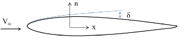
immersed body and at different location of the fluid domain.

Figure 3.2. Schematic for mathematical formulation of steady flow over an immersed body

For the problem to be well posed, the following boundary conditions are required to solve

Eqs. 3.10–3.12:

 2 boundary conditions on v_x in x-direction

 2 boundary conditions on v_x in y-direction

(48)

35  2 boundary conditions on vy in y-direction

 1 boundary condition on p in x-direction

 1 boundary condition on p in y-direction

The boundary conditions at the solid surface of the immersed body refer to the no-slip

condition which states that the fluid must stick to the surface of the immersed body due to

viscous effects. Referring to Fig. 3.2 and considering the surface of the solid object as( , )x y ,

these boundary conditions are expressed mathematically in Eqs. 3.13 and 3.14.

0 ,

x

v  at x y  (3.13)

0 , y

v  at x y  (3.14)

The boundary conditions at the far field state that the velocity must be equal to the

freestream velocity given that the flow in this region is not affected by the interaction with the

immersed body. Mathematically, these boundary conditions are show in Eqs. 3.15 and 3.16.

0

0 0 x

x

v V at y for x L

or v

at y for x L

y



    

 _ _{ } _{ }



(3.15)

0 0 y

v  at y  for  x L (3.16)

The boundary conditions at the entrance or inlet of the computational domain state the

velocity must be equal to the freestream velocity. Mathematically, these boundary conditions are

show in Eqs. 3.17 and 3.18.

0 0

x

(49)

36

0 0 0 y

v  at x for   y (3.18)

Lastly, pressure boundary conditions are prescribed on the domain. Mathematically, they

are expressed in Eqs. 3.19 and 3.20.

0

PP_ at xL for   y (3.19)

0

PP_ at y  for  x L (3.20)

3.3. Unsteady Flow over an Immersed Body Mathematical Formulation

This section presents the mathematical relationships that govern the unsteady fluid

motion over an arbitrary body immersed on a fluid domain.

The conservation of mass and momentum in their most general vector form are presented

in Eqs. 3.21 and 3.22.

( V) 0

t

 _

 _{  } _

 (3.21)

Conservation of momentum:

'_ij

DV

g p Dt

      (3.22)

where

 

ij

2

' for , , 1, 2, 3

3 0 1 j i ij j i ij V V

V i j k

(50)

37 3.3.2.Assumptions

1) The flow is incompressible.

2) The flow is 2-D.

3) The flow is laminar with Reynolds number less than Reynolds critical number which is

equal to 5×105.

4) The properties of the fluid remain constant across a small differential element.

5) Buoyancy terms are neglected.

6) The fluid is Newtonian meaning that there is linear relationship between shear and strain.

Considering the assumptions stated previously, the conservation equations are expanded

from the general vector form and are presented in Cartesian coordinates in Eqs. 3.24–3.26 [44].

Conservation of ass:

0 y

x v

v

t x y

  

 _ _ _

   (3.24)

Conservation of momentum:

x-direction:

2 2

1

x x x x x

x y

v v v p v v

v v

t x y  x  x y

 

     

     _  _

    _   _ (3.25)

y-direction:

2 2

1

y y y y y

x y

v v v p v v

v v

t x y  y  x y

 

 _  _  _{ }  _  _

 

Modal Characterization and Structural Dynamic Response of a Crane Fly Forewing

ScholarWorks@UNO

ScholarWorks@UNO

Modal Characterization and Structural Dynamic Response of a

Modal Characterization and Structural Dynamic Response of a

Crane Fly Forewing

Crane Fly Forewing

Modal Characterization and Structural Dynamic Response of a Crane

Fly Forewing

Acknowledgement

Table of Contents

Nomenclature

List of Figures

List of Tables

Abstract

CHAPTER 1. INTRODUCTION

1.1.

Flow over Immersed Bodies



1.2.

Insect Flight Kinematics

1.3.

Micro Air Vehicles

1.4.

Literature Survey

1.5.

Motivation and Objective of Study

CHAPTER 2. MATERIALS AND METHODS

2.1.

Specimen Characterization

2.2.

Micro-CT Scan

2.3.

Computational Model

















CHAPTER 3. MATHEMATICAL MODELING

3.1.

Vacuum Analysis Mathematical Formulation

3.2.

Steady Flow over an Immersed Body Mathematical Formulation

 

3.3.

Unsteady Flow over an Immersed Body Mathematical Formulation

 