HiGlass: web based visual exploration and analysis of genome interaction maps

S O F T W A R E

Open Access

HiGlass: web-based visual exploration and

analysis of genome interaction maps

Peter Kerpedjiev

, Nezar Abdennur

, Fritz Lekschas

, Chuck McCallum

, Kasper Dinkla

, Hendrik Strobelt

,

Jacob M. Luber

, Scott B. Ouellette

, Alaleh Azhir

, Nikhil Kumar

, Jeewon Hwang

, Soohyun Lee

, Burak H. Alver

,

Hanspeter Pfister

, Leonid A. Mirny

, Peter J. Park

and Nils Gehlenborg

Abstract

We present HiGlass, an open source visualization tool built on web technologies that provides a rich interface for rapid, multiplex, and multiscale navigation of 2D genomic maps alongside 1D genomic tracks, allowing users to combine various data types, synchronize multiple visualization modalities, and share fully customizable views with others. We demonstrate its utility in exploring different experimental conditions, comparing the results of analyses, and creating interactive snapshots to share with collaborators and the broader public. HiGlass is accessible online at

http://higlass.ioand is also available as a containerized application that can be run on any platform.

Keywords:Hi-C, Data visualization, Chromosome conformation, Genomics

Background

The development of chromosome capture assays meas-uring the spatial contacts between two or more regions of the genome is essential for elucidating how the struc-ture and dynamics of the genome affect gene regulation and cellular function [1, 2]. Genome-wide maps of chromosomal interactions obtained by techniques such as Hi-C have revealed features of genome organization such as compartmentalization, i.e., spatial segregation of active and inactive regions of the genome, topologically associating domains (TADs), and associated peaks of contact frequency (often referred to as loops) [1, 3–5]. Hi-C maps have helped implicate changes in genome organization in a variety of disorders, including acute lymphoblastic leukemia [6], colorectal cancer [7], and limb development disorders [8]. More fundamentally, they provide insights into the mechanisms by which genome conformation structures arise, are maintained, and change over time [9–11]. Major efforts like the 4D Nucleome Network and the ENCODE project are gener-ating such data at large scale across different cell lines and conditions with the aim of understanding the mech-anisms that govern processes such as gene regulation

and DNA replication as well as to cross-validate the results from different experimental assays [12,13].

Despite the large amounts of generated Hi-C data, major challenges remain in (i) identifying known fea-tures unambiguously [14]; (ii) discovering new features; (iii) establishing relationships between Hi-C features and known (epi)genetic profiles; (iv) establishing the effects of various genetic, biochemical, and physical perturbations on chromatin organization, assessing meaningful differ-ences between cell types [15], and assessing changes across the cell cycle and along differentiation pathways [16]. These challenges necessitate the development of methods to visually explore, compare, and share not only the raw data but also related datasets and derived analysis results. An effective visualization platform needs to meet the following criteria: (1) Provide researchers with the means to explore their data and look for patterns that may help to interpret the results of experiments and generate hypotheses. (2) Enable efficient comparison by juxtapos-ition or other means of different samples or condjuxtapos-itions and integration of both similar and heterogeneous data types. (3) Allow researchers to overlay computationally derived annotations to visually validate analytical results as well as to compare the outputs of different data pro-cessing pipelines. (4) Enable sharing of results with collab-orators and the public. And crucially, an effective platform does this all in a fast, intuitive, and accessible manner. * Correspondence:[email protected]

1_{Department of Biomedical Informatics, Harvard Medical School, Countway}

Library, 10 Shattuck St, Boston, MA 02115, USA

Full list of author information is available at the end of the article

To obtain genome conformation capture maps, raw Hi-C sequencing data are processed to identify proximity ligation events representing captured contacts between genomic loci, which are then binned to form contact matrices [17–19]; see Lajoie et al. [20] and Ay and Noble [21] for reviews of Hi-C data processing. The discovery and elucidation of genome organizational principles and mechanisms, however, also require sophisticated visual tools for exploring features relevant at scales ranging from tens to millions of base pairs [18,22,23]. Given the multi-scale features of genome organization, it is crucial that such visualization tools support comparison across mul-tiple scales and conditions as well as integration with add-itional genomic and epigenomic data. Existing tools provide different ways of displaying contact frequencies, such as rectangular heatmaps, triangular heatmaps, arc plots, or circular plots, and different degrees of interactiv-ity ranging from static plotting to interactive zooming and panning, as well as different degrees of integration with other genomic data types [18,24–29]. While tools such as Juicebox [18] and Genome Contact Map Explorer [30] provide synchronized exploration of multiple contact maps, they lack an interface for dynamically arranging the views of several Hi-C datasets, and customizing the levels of synchronization between loci, zoom levels, and samples. Furthermore, none provide an interface for continuous panning and zooming of the sort popularized by web-based geographical and road maps.

To address these shortcomings, we created HiGlass, an open source, web-based application designed to support multiscale contact map and genomic data track visualization across multiple resolutions, loci, and condi-tions (http://higlass.io; Additional file 1: Supplementary methods). HiGlass was built with an emphasis on usabil-ity. It provides an interface for continuous panning and zooming across genome-wide data. To facilitate compari-son and exploration, HiGlass introduces the concept of

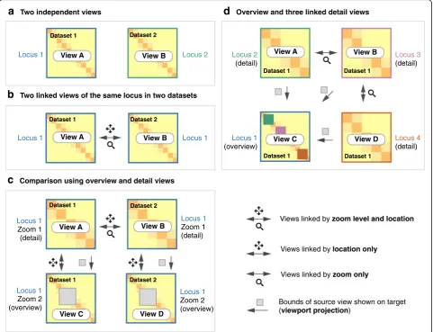
“composable linked views” for genomic data visualization (Fig.1).Each view in HiGlass is a collection of 1D and 2D tracks sharing common genomic axes. Views can be filled with data tracks, resized, arranged spatially, and linked to synchronize their axes by location or zoom level. This ap-proach enables users to interactively compose the layout, content, and synchronization of locus, zoom level, and other properties across multiple views (Fig.1). By creating, sizing, arranging, and linking individual views, users can create custom compositions ranging from the juxtapos-ition of two or more heatmaps to sophisticated arrange-ments of views containing matrices, tracks, and“viewport projections” mapping the extents of one view inside another (Figs.1,4, and5, Additional file1: Figure S1). We demonstrate how HiGlass has been used to detect and analyze novel features in Hi-C data and to visualize, valid-ate, and compare tools for detection of known features.

Multiple views within the same browser window, with synchronized panning and zooming, allow fast compari-son of Hi-C maps for different samples/conditions. Views can, in the simplest case, be arranged to show the same location at the same zoom level across multiple samples (Figs. 2 and 3). In other cases, the investigator may wish to view multiple loci within the same sample (Fig. 1band Additional file1: Figure S2). More complex arrangements can pair views with different zoom levels in a context–detail arrangement (Figs. 4 and 5) [31]. View compositions serve to display data at multiple scales, to corroborate observations with other types of evidence and to facilitate comparisons between experiments. As a web-based tool, HiGlass also supports storing and sharing of view compositions with other investigators and the public via hyperlinks. The tool can be used to access selected public datasets at http://higlass.io or it may be run locally and populated with private data using a provided Docker container. It can also be embedded within other applications to provide a component for displaying Hi-C or other genomic data [32].

Results

Exploring and comparing different experimental conditions

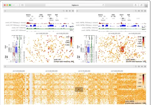
ΔNipbl and navigated to the region between chr14:50 Mb and chr14:70 Mb (Fig.4, bottom). Adding H3K4me3 and H3K27ac ChIP-seq signal tracks revealed that these marks, while similar between conditions, correlate more strongly with the compartmentalization pattern in ΔNipbl. Finally, we used a viewport projection to mark the position of the bottom views relative to the top, resulting in the complete view composition shown in Fig.4. This interactive visual re-capitulation of key results from Schwarzer et al [33]. illus-trates how synchronized navigation across loci and resolutions by linking views between multiple conditions fa-cilitates the exploration of the complex effects of global per-turbations on chromosome organization at multiple scales.

Using the same view composition we noticed the appearance of a new feature, small dark patches (“blotches”) away from the diagonal in the ΔNipbl

condition. To investigate these patches we created a new composition containing an overview and two zoom- and location-linked detail views (Fig. 5). By using the over-view to find patches and comparing them using the de-tail views, we established that they are more enriched in the mutant condition than in the wild type, that they represent strengthened interactions between pairs of short active regions (type A compartment), and that they tend to be aligned with annotations of long multi-exonic genes. Including RNA-seq and ChIP-seq tracks let us see that the genes which align with these patches are virtu-ally always transcriptionvirtu-ally active. These observations are reminiscent of a recent ultra-high-resolution Hi-C study in mouse embryonic stem and neural cells, where the long-range contact enrichment between pairs of expressed genes was found to correlate with both

a

d

View C View A Locus 1

Locus 1

Zoom 1 (detail)

Locus 1

Zoom 2 (overview)

Locus 1

Zoom 2 (overview)

Locus 1 Locus 1

(overview)

Locus 1

Zoom 1 (detail)

Locus 2 Locus 2

(detail)

Locus 3 (detail)

Locus 4

(detail)

b

c

Views linked by zoom level and location

Views linked by location only

Bounds of source view shown on target (viewport projection)

Views linked by zoom only View B

View B

View D

Dataset 1

Dataset 1

Dataset 1

Dataset 1

Dataset 2

Dataset 2

Dataset 1 Dataset 1

Dataset 1 Dataset 1

Dataset 2

Dataset 2

View A

View A View B

View C

View B View A

View D

expression level and the number of exons, and agrees with similar strengthened patterns observed after deg-radation of cohesin in a human cell line [35, 36]. Not only do composable linked views provide convincing support that the absence of cohesin loading leads to strengthening of global genome compartmentalization, but they also hint that, at finer scales, long range and inter-chromosomal contact enrichment and its response to cohesin loss are influenced by transcriptional parame-ters such as expression output and splicing activity.

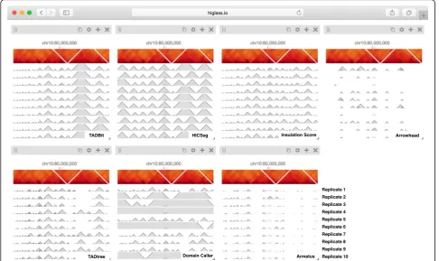
Comparing the results of feature callers

Analysis of genomic data usually involves identification and annotation of various “features” that range from calling sequence variants to detecting complex patterns of interactions in Hi-C maps. Often, the first step in characterizing the quality of a caller is a visual inspection to verify that the regions it annotates match the expecta-tions of the human analysts. In the case of ChIP-seq data, for example, peak callers identify regions where proteins bind [37] and an analyst would verify that the regions contain an elevated number of read counts relative to the surrounding regions. In Hi-C data, topologically as-sociated domain (TAD) callers identify regions of

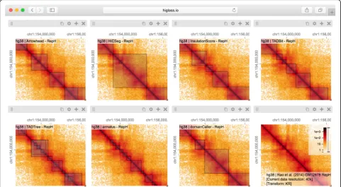
increased contact frequency in contiguous loci (e.g., along the diagonal in a Hi-C map) [3,4]. In contrast to 1D peak callers, TAD callers demarcate square regions of interest in a Hi-C map. This makes comparison more complicated as the results often need to be placed next to each other, rather than simply stacked on top of each other. Results from multiple callers run on multiple replicates further complicate the task of comparison.

same scale as the larger compartment features, but also overlap with compartmental transitions (Fig. 2). Down-stream analysis based on such TAD calls should therefore consider whether phenomena attributed to TADs can also be attributed to other features of Hi-C.

In addition to the differences between TAD calls among different callers, there are differences in the calls produced by a single TAD caller on different replicates. Such differ-ences may be attributable to variations in signal-to-noise (e.g., quality and depths of different sequencing runs and differences in library complexity between replicates). Fur-thermore, by looking at the results of seven different TAD callers among ten experiments we can see that consistency within a caller does not imply consistency between callers. Such views also reveal more subtle differences. Some callers, for example, partition nearly all of the genome into a con-tiguous sequence of “TADs” (HiCseg [38], insulationScore [39], and TADbit [40]), while others (Arrowhead [5], TAD-Tree [41], domainCaller [3], and Armatus [42]) call discon-tinuous intervals, and some methods allow for overlap and/ or nesting [14]. Such differences raise meaningful questions about what data patterns are used to define TADs in

different studies, how robustly different algorithms can cap-ture any given pattern type, and how the findings from one study can be translated to those of another. These issues are further underlined by recent experimental perturbations of chromatin architectural factors, such as the Nipbldeletion study above, which reveal that segmental annotations based solely on local contact enrichment cannot all be attributed to the same organizational process inside the nucleus and that standard Hi-C maps reflect an interplay of distinct dynamic processes averaged over a cell population.

Creating interactive snapshots of genome-wide data

publications, the extents of these plots are limited by the space and resolution available on the printed page. This compels authors to show one or two loci that most clearly demonstrate the effect they are describing. The original data are archived in repositories such as the Gene Expres-sion Omnibus (GEO). A user who wishes to explore add-itional examples or view the data using a different visual representation requires a non-trivial human effort to a) lo-cate the data in the appropriate repository, b) establish which files correspond to which figures, and c) prepare, convert, and load the data into a genome browser or viewer. This arrangement hinders communication, repro-ducibility, and further analysis by dissociating the raw genome-wide data from the publication describing it.

With HiGlass, authors can produce links to interactive figures that can be shared with collaborators or the public. These links point to HiGlass view compositions that can show all of the genome-wide data used to produce a fig-ure. These compositions are centered on one or more loci

but can be navigated to other locations. Generating a link to a view composition stores all of the information neces-sary to reproduce it, including the data sources, track types, and synchronization links on the hosting server. This“view config”can also be stored as a file that can be shared with collaborators. Similar functionality was pio-neered by the UCSC Genome Browser [43], where users could create “Track Hubs” hosting their own data and then share session links to genome browser views incorp-orating their data. Similarly, HiGlass users can run their own server locally and share links pointing to local data as well as data hosted on remote servers.

space-constrained URL, we can include more metadata about how the tracks are styled and linked, the data sources, and the synchronization options. This JSON state representation can either be saved locally or stored in HiGlass’s database and shared as a link to an interactive figure (Figs.2,3,4, and5). By capturing the current com-position and storing its complete state on the server, we create the opportunity to integrate HiGlass with tools for documenting and exploring the provenance of the com-position to better understand the steps that the analyst took to reach their conclusions [44].

Feature overview and comparison with other viewers

The major strengths of HiGlass are smooth navigation, multi-view comparison, comprehensive selection of track types, and containerized deployment. Of the existing browsers, only HiGlass and Genome Contact Map

Explorer (GCME) provide a continuous interface for panning and zooming across loci and resolutions. Other tools, such as Juicebox, Juicebox.js [45], the Washington University Epigenome Browser (WUEB), and the 3D Genome Browser show data at fixed discrete zoom levels. To compare data, Juicebox, Juicebox.js, GCME, and HiGlass offer the opportunity to place heatmaps side by side and navigate multiple Hi-C maps simultan-eously. Of these, only HiGlass lets users select which heatmaps to synchronize or whether to synchronize by location, zoom, or both. This is critical for the creation of task-specific view compositions, for example, to sup-port overview and detail or multiple comparisons. Fur-thermore, no other tools let users establish connections between views (viewport projections) so as to display the location of one view within another (Figs.4and5).

already supports horizontal triangular heatmaps (Fig.5), vertical triangular heatmaps, and 2D heatmaps (Figs. 3, 4, and 5) for viewing Hi-C data as well as tracks for showing 2D annotations (Figs.2 and 3). This is in con-trast to other viewers such as Juicebox, Juicebox.js, and GCME, which display only 2D heatmaps, or WUEB and the 3D Genome Browser, which only display horizontal triangular heatmaps. Heatmaps in HiGlass are highly configurable. Color scales can be synchronized, tuned, and adjusted to display both linearly and logarithmically scaled data, an option also present only in GCME. Such features are crucial because the dynamic range of intra-chromosomal contact frequency spans several or-ders of magnitude. Genomic signal tracks can be dis-played using lines, bars, or points. Other track types, such as gene annotations, rotated 2D annotations (Fig. 5), and generic 1D annotations, are also directly sup-ported. HiGlass supports selectable synchronized scaling between values in different tracks as well as the ability to fix heatmap color scales to a defined data range. It supports SVG export as well as JSON view config and link export for sharing (see the “Creating interactive snapshots of genome-wide data”section).

For deployment, we provide a Docker container for HiGlass, which can be run locally and populated with pri-vate or shared data (Fig.6). This makes it possible for indi-viduals to view local files or for laboratories to create instances shared within an internal network. Such instances can be used to isolate both data and shared interactive fig-ures from the public. Laboratories can also set up public in-stances to share data and figures outside of the local network. The ability to set up public and private instances is also available for the Washington University Epigenome Browser but absent from other tools. Because Juicebox and Juicebox.js can load remote files, similar functionality can be approximated by controlling data access at its point of storage. Without a database, however, it is difficult to obtain lists of available tracks and their associated visual encodings from within the viewer itself. HiGlass makes it possible to not only collect sets of tracks locally but also to connect to and obtain tracks from any number of different remote in-stances, such as the one athttp://higlass.io.

Conclusions

Using HiGlass to create the linked views shown in Figs. 2and3enabled us to interactively explore the data gen-erated by Schwarzer et al. across different conditions, zoom levels, and loci [46]. This gave us not only a clearer understanding of the results but also the ability to see them in a genic context, and also allowed us to find unexpected patterns, relate them to histone patterns and gene expression, and rapidly gather observations to be used in generating new hypotheses. We used a

different composition of views to show and compare the results of seven different TAD callers in a single window [14]. This let us compare the variation among different TAD callers, and of the same caller, across different rep-licates (Fig.3), as well as with the original data that the calls were generated from (Fig. 2). These figures highlighted the inconsistency in the results between sep-arate TAD callers, further emphasizing the algorithmic challenges and underscoring the need for visual inspec-tion of these results. Finally, we provide links to fully navigable, interactive versions of each of these figures. This gives readers the freedom to explore the full extent of the data outside of the confines of the printed page.

The multiscale nature of Hi-C data demands visualization at a wide range of zoom levels. Its size necessitates piece-wise loading of small chunks of data. While genome browsers pioneered multiscale, genome-wide views of 1D data and other tools extended the notion to Hi-C data, the methods of comparison have largely been limited to either a simple vertical tiling of horizontal data tracks or a split-ting of Hi-C contact maps along the diagonal. With HiGlass, we have generalized the approach to comparison and extended it beyond simple stacking or two-way splits. We have introduced operations for linking views by loca-tion and/or zoom level and for projecting viewports across views. The tool that we have developed, while originally de-signed for Hi-C data, is a data-agnostic multi-dimensional viewer. Our public demo (http://higlass.io) demonstrates how HiGlass can be used as a standalone viewer to display 1D genomic data [47] while simultaneously providing the same view composition operations for comparison across loci and resolutions.

Having effective tools for comparing genomic data highlights the challenge of organizing such data so that it can be easily found and displayed. Projects such as ENCODE and 4D Nucleome are generating Hi-C data, annotating it with metadata, and making them available to the broader public. Efforts like UCSC Genome Browser’s track hubs paved the way for remote genomic data hosting, integration, and visualization. However, there is a need to make it easier for researchers to find and integrate the data that helps answer their biological questions. Future goals in that direction include adding extended metadata to HiGlass data servers and imple-menting standardized APIs to identify, describe, and query genomic data sets. With more available data, we can take advantage of HiGlass’s extensible architecture to create new ways of exploring, comparing, and inter-preting multi-scale experimental results.

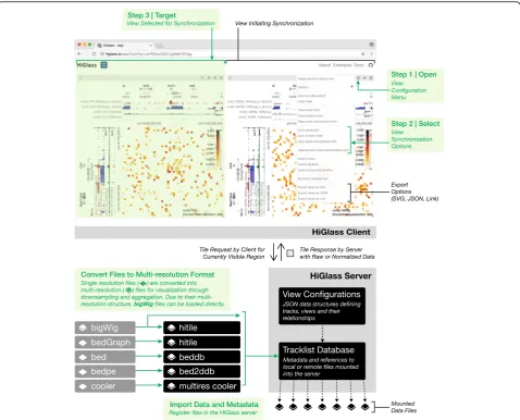
Methods

the server is written in Python. The client is responsible for arranging tracks and views and requesting data from the ser-ver. The server loads data from files in small chunks called

“tiles”and sends them back to the client upon request.

Data are organized according to zoom level using an aggregation or downsampling function

We maintain data at different pre-computed resolutions and when the user zooms in, HiGlass displays higher resolution data. This approach is also employed by web-based map visualization tools such as Google Maps and Open Street Maps. The UCSC Genome Browser and the Integrative Genome Viewer pioneered this ap-proach for genomic data [48, 49]. For contact matrices which are generated by binning lists of contacts, creating

lower resolution matrices simply requires binning with a larger bin size. The bin sizes used by HiGlass are typic-ally multiples of the powers of 2, starting from the high-est resolution data (e.g., for 1 K data, bin sizes would be 1 K, 2 K, 4 K, …, 16.384 M) but can also be set to arbitrary multiples of the highest resolution. The lower zoom level corresponds to the minimum bin size which can fit 1/256th of the width of the matrix. Lower-resolution matrices of counts can also be created by downsampling or

“aggregating” higher resolution matrices. In this operation, adjacent pairs of higher resolution bins are merged by sum-ming their values.

merged by summing their values. In so doing, we maintain a separate array of counts for the number of missing values encountered. This allows us to compute average values when displaying lower resolution data.

For categorical data, downsampling requires discarding values. Values to be discarded are chosen according to an“importance value”. This importance value can be ei-ther user-defined or set randomly. A more intelligent importance value can consider a relevant property of the data when deciding which should be visible at lower resolution. For example, for gene annotation tracks, we use a custom importance value based on the number of citations referencing a particular gene. Genes which are well studied and referenced often in the literature, such as TP53 and TNF, remain visible as the user zooms out. More obscure genes appear only when there is enough space. For 2D annotations, we use the size of the anno-tation as an importance value so that larger annoanno-tations are visible when zoomed out and smaller annotations only appear at high resolution.

Tiles break down large datasets into manageable chunks that can be sent from the server to the client

A tile, in the context of HiGlass, is the data available for a given location and zoom level. This is analogous to the tiles used by online maps to show the portion of the map that is visible in the current viewport (Additional file 1: Figure S7). In the case of Hi-C data, which can be represented as a matrix for any given resolution, a tile consists of a 256 × 256 slice of the matrix.

Zoom levels correspond to the different levels of reso-lution. The highest zoom level, zmax, corresponds to the highest resolution data. Each lower zoom level (z-1), cor-responds to data at half the resolution of the previous level (r/2). The data at zoom level 0 must be at a reso-lution low enough such that the whole genome can be fit into one 256 × 256 tile. This yields an expression for calculating the maximum zoom level for data with a starting (highest) resolution of r0and a genome size of g:

zmax¼ log2ðg= 256r0Þ

For quantitative 1D genomic data, such as RNA-seq or ChIP-seq or any other coverage-based measure, a tile con-sists of the data from a 1024-base-pair region of the gen-ome. The concepts behind the resolution and zoom levels are the same as for 2D data except that instead of a tile corresponding to a square of the matrix at a resolution, it corresponds to a segment of the genome at a given reso-lution. For qualitative data, the server returns all entries which intersect the length or area of the tile.

In both 1D and 2D data, the lowest resolution is shown at zoom level 0. Given a zoom level, z, the tile

visible at genome locationlgcan be calculated by consid-ering the width of a tile:tw= r0* 2z

tp ¼lg=tw

Genomes, being composed of chromosomes, do not have absolute positions. To get around this, we impose a chromosome ordering for every dataset that is viewable in HiGlass. This must be specified when the data are preprocessed.

HiGlass stores multi-scale datasets

Due to the limitations of the visible display, a fixed amount of data can be shown in any given area. For a window that is 1024 × 1024 pixels in size, the maximum resolution that the human genome can be shown at is approximately 3 million base pairs/pixels. Fetching all the data from the server is wasteful and unnecessary. We therefore use file formats that store Hi-C and gen-omic data at multiple resolutions. For Hi-C data, we use the cooler (http://github.com/mirnylab/cooler) format and for genomic data we support the widely used big-Wig format [49]. Both support the basic query format of resolution/location. When creating multi-resolution cooler files, we create resolutions that are multiples of the powers of 2 in order to create a smooth transition as the user zooms in and out of the data. While this does increase the size of the data (Additional file1: Table S1), multiple resolutions are necessary to limit the amount of data that needs to be retrieved from the server when viewing large portions of the contact map.

The HiGlass server fetches data from files and returns it to the client on demand

The HiGlass server is the interface between the client and the data (Fig. 6, Additional file 1: Supplementary methods). It receives requests for data (tiles) from the client, opens the data files, and returns only the data requested. This minimizes the amount of data that needs to be sent across the network and in turn lowers the time required to load the data for a given location. Of the 2,770,448 tile requests to our public server at http:// higlass.io between February 2017 and July 2018, 2,677,856 (> 96.7%) were fetched with a latency of less 0.5 s, a limit beyond which the rates of “observation, generalization and hypothesis significantly decreased” in a controlled user study [50].

Availability and requirements

HiGlass is available as a Docker container and can thus be run on any operating system as long as it supports the Docker platform. An active internet connection is required to fetch the Docker container as well as the Javascript source files. Documentation for how to run HiGlass can be found athttp://docs.higlass.io.

Additional file

Additional file 1:Figures S1.–S7. Table S1.Supplementary material, and Supplementary references. (PDF 755 kb)

Acknowledgements

We thank Francois Spitz, Wibke Schwarzer, Aleksandra Pekowska, Mattia Forcato, and Francesco Ferrari for providing the data presented in this paper. We thank Geoffrey Fudenberg for feedback on the manuscript. We also acknowledge important suggestions and feedback from members of the Park Lab at Harvard Medical School, the Mirny Lab at MIT, and the Dekker Lab at University of Massachusetts Medical School as well as members of 4D Nucleome Data Coordination and Integration Center who provided input and feedback.

Funding

This project was made possible by funding from the National Institutes of Health (U01 CA200059, R00 HG007583, and U54 HG007963).

Availability of data and materials

This paper used data from two published studies, the data for which are on GEO. Note that the data from Rao et al. [5] were processed according to the TAD-calling procedures described in Forcato et al. [14].

1. Schwarzer et al. [33], GEO accession GSE93431https:// www.ncbi.nlm.nih.gov/geo/query/acc.cgi?acc=GSE93431 2. Rao et al. [5], GEO accession GSE63525

https://www.ncbi.nlm.nih.gov/geo/query/acc.cgi?acc=GSE63525

The source code for HiGlass can be found in five complementary GitHub repositories. All of the source code is licensed under the open source MIT License.

https://github.com/hms-dbmi/higlass- The client side Javascript viewer component (doi: 10.5281/zenodo.1308881) [51].

https://github.com/hms-dbmi/higlass-website- A scaffold web site that incorporates the viewer (doi: 10.5281/zenodo.1308901) [52]

https://github.com/hms-dbmi/higlass-server- The server we created for serving multi-resolution data (doi: 10.5281/zenodo.1308945) [53]

https://github.com/hms-dbmi/higlass-docker- A ready-to-deploy Docker container with installations of the previous three components (doi: 10.5281/ zenodo.1308947) [54]

https://github.com/hms-dbmi/higlass-manage- A set of commands for easy deployment and management of the Docker container (doi: 10.5281/ zenodo.1308949) [55]

Hi-C matrices need to be stored in the cooler format (https://github.com/ mirnylab/cooler/).

Comprehensive documentation for HiGlass can be found athttp://docs.higlass.io

Authors_’contributions

PK and NG conceived the research. PK, NA, and NG wrote the manuscript with input from LAM, PJP, and BHA. PK, NA, FL, and CM wrote the software with help from KD, HS, JML, SO, AA, NK, JH, and SL. BHA, HP, LAM, and PJP provided valuable input and advice for the project. All authors read and approved the final manuscript.

Ethics approval and consent to participate

Not Applicable.

Consent for publication

Not Applicable.

Competing interests

The authors declare that they have no competing interests.

Publisher’s Note

Springer Nature remains neutral with regard to jurisdictional claims in published maps and institutional affiliations.

Author details 1

Department of Biomedical Informatics, Harvard Medical School, Countway Library, 10 Shattuck St, Boston, MA 02115, USA.2_{Computational and Systems} Biology Program, MIT, Cambridge, USA.3School of Engineering and Applied Sciences, Harvard University, Cambridge, MA, USA.4_{Bioinformatics and} Integrative Genomics Program, Harvard Medical School, Boston, MA, USA. 5_{Department of Physics, MIT, Cambridge, USA.}6_{Institute for Medical}

Engineering and Science, MIT, Cambridge, USA.

Received: 22 November 2017 Accepted: 18 July 2018

References

1. Lieberman-Aiden E, van Berkum NL, Williams L, Imakaev M, Ragoczy T, Telling A, et al. Comprehensive mapping of long-range interactions reveals folding principles of the human genome. Science. 2009;326:289–93. 2. Dekker J, Marti-Renom MA, Mirny LA. Exploring the three-dimensional

organization of genomes: interpreting chromatin interaction data. Nat Rev Genet. 2013;14:390–403.

3. Dixon JR, Selvaraj S, Yue F, Kim A, Li Y, Shen Y, et al. Topological domains in mammalian genomes identified by analysis of chromatin interactions. Nature. 2012;485:376_–80.

4. Nora EP, Lajoie BR, Schulz EG, Giorgetti L, Okamoto I, Servant N, et al. Spatial partitioning of the regulatory landscape of the X-inactivation centre. Nature. 2012;485:381–5.

5. Rao SSP, Huntley MH, Durand NC, Stamenova EK, Bochkov ID, Robinson JT, et al. A 3D map of the human genome at kilobase resolution reveals principles of chromatin looping. Cell. Elsevier. 2014;159:1665–80.

6. Hnisz D, Weintraub AS, Day DS, Valton A-L, Bak RO, Li CH, et al. Activation of proto-oncogenes by disruption of chromosome neighborhoods. Science. 2016;351:1454–8.

7. Seaman L, Chen H, Brown M, Wangsa D, Patterson G, Camps J, et al. Nucleome analysis reveals structure-function relationships for colon cancer. Mol Cancer Res. 2017. Available from:https://doi.org/10.1158/1541-7786. MCR-16-0374

8. Lupiáñez DG, Kraft K, Heinrich V, Krawitz P, Brancati F, Klopocki E, et al. Disruptions of topological chromatin domains cause pathogenic rewiring of gene-enhancer interactions. Cell. Elsevier. 2015;161:1012_–25.

9. Sanborn AL, Rao SSP, Huang S-C, Durand NC, Huntley MH, Jewett AI, et al. Chromatin extrusion explains key features of loop and domain formation in wild-type and engineered genomes. Proc Natl Acad Sci U S A. 2015;112: E6456_–65.

10. Fudenberg G, Imakaev M, Lu C, Goloborodko A, Abdennur N, Mirny LA. Formation of chromosomal domains by loop extrusion. Cell Rep. 2016;15: 2038–49.

11. Zuin J, Dixon JR, van der Reijden MIJA, Ye Z, Kolovos P, Brouwer RWW, et al. Cohesin and CTCF differentially affect chromatin architecture and gene expression in human cells. Proc Natl Acad Sci U S A. 2014;111:996–1001. 12. ENCODE Project Consortium. An integrated encyclopedia of DNA elements

in the human genome. Nature. 2012;489:57_–74.

13. Dekker J, Belmont AS, Guttman M, Leshyk VO, Lis JT, Lomvardas S, et al. The 4D nucleome project. Nature. 2017;549:219–26.

14. Forcato M, Nicoletti C, Pal K, Livi CM, Ferrari F, Bicciato S. Comparison of computational methods for Hi-C data analysis. Nat Methods. 2017;14:679_–85. 15. Schmitt AD, Hu M, Jung I, Xu Z, Qiu Y, Tan CL, et al. A compendium of

chromatin contact maps reveals spatially active regions in the human genome. Cell Rep. 2016;17:2042–59.

16. Gibcus JH, Samejima K, Goloborodko A, Samejima I, Naumova N, Kanemaki M, et al. A pathway for mitotic chromosome formation. Science. 2018;359. 6376:eaao6135.

18. Durand NC, Robinson JT, Shamim MS, Machol I, Mesirov JP, Lander ES, et al. Juicebox provides a visualization system for Hi-C contact maps with unlimited zoom. Cell Syst. 2016;3:99–101.

19. Servant N, Varoquaux N, Lajoie BR, Viara E, Chen C-J, Vert J-P, et al. HiC-Pro: an optimized and flexible pipeline for Hi-C data processing. Genome Biol. 2015;16:259.

20. Lajoie BR, Dekker J, Kaplan N. The Hitchhiker’s guide to Hi-C analysis: practical guidelines. Methods. 2015;72:65_–75.

21. Ay F, Noble WS. Analysis methods for studying the 3D architecture of the genome. Genome Biol. 2015;16:183.

22. Gehlenborg N, O_’Donoghue SI, Baliga NS, Goesmann A, Hibbs MA, Kitano H, et al. Visualization of omics data for systems biology. Nat Methods. 2010;7: S56_–68.

23. Nielsen CB, Cantor M, Dubchak I, Gordon D, Wang T. Visualizing genomes: techniques and challenges. Nat Methods. 2010;7:S5–15.

24. Wang Y, Zhang B, Zhang L, An L, Xu J, Li D, et al. The 3D Genome Browser: a web-based browser for visualizing 3D genome organization and long-range chromatin interactions. bioRxiv. 2017:112268. Available from:http:// biorxiv.org/content/early/2017/02/27/112268. Accessed 2 Mar 2017. 25. Zhou X, Lowdon RF, Li D, Lawson HA, Madden PAF, Costello JF, et al.

Exploring long-range genome interactions using the WashU Epigenome Browser. Nat Methods. 2013;10:375–6.

26. Akdemir KC, Chin L. HiCPlotter integrates genomic data with interaction matrices. Genome Biol. 2015;16:198.

27. Yard_ımc_ıGG, Noble WS. Software tools for visualizing Hi-C data. Genome Biol. 2017;18:26.

28. Martin JS, Xu Z, Reiner AP, Mohlke KL, Sullivan P, Ren B, et al. HUGIn: Hi-C unifying genomic interrogator. Bioinformatics. 2017;33:3793–5.

29. Calandrelli R, Wu Q, Guan J, Zhong S. GITAR: an open source tool for analysis and visualization of Hi-C data. bioRxiv. 2018:259515. Available from:https:// www.biorxiv.org/content/early/2018/05/08/259515. Accessed 24 May 2018. 30. Kumar R, Sobhy H, Stenberg P, Lizana L. Genome contact map explorer: a

platform for the comparison, interactive visualization and analysis of genome contact maps. Nucleic Acids Res. 2017; Available from:https://academic.oup. com/nar/article-lookup/doi/10.1093/nar/gkx644. Accessed 29 Aug 2017. 31. Cockburn A, Karlson A, Bederson BB. A review of overview+detail, zooming,

and focus+context interfaces. ACM Comput Surv. 2009;41:2:1–2:31. 32. Lekschas F, Bach B, Kerpedjiev P, Gehlenborg N, Pfister H. HiPiler: visual

exploration of large genome interaction matrices with interactive small multiples. IEEE Trans Vis Comput Graph. 2017. Available from:https://doi. org/10.1109/TVCG.2017.2745978

33. Schwarzer W, Abdennur N, Goloborodko A, Pekowska A, Fudenberg G, Loe-Mie Y, et al. Two independent modes of chromatin organization revealed by cohesin removal. Nat Res. 2017. Available from:https://doi.org/ 10.1038/nature24281

34. Fudenberg G, Abdennur N, Imakaev M, Goloborodko A, Mirny LA. Emerging evidence of chromosome folding by loop extrusion. Cold Spring Harb Symp Quant Biol. 2018. Available from:https://doi.org/10.1101/sqb.2017.82. 034710

35. Bonev B, Mendelson Cohen N, Szabo Q, Fritsch L, Papadopoulos GL, Lubling Y, et al. Multiscale 3D genome rewiring during mouse neural development. Cell. 2017;171:557–72. e24

36. Rao SSP, Huang S-C, Glenn St Hilaire B, Engreitz JM, Perez EM, Kieffer-Kwon K-R, et al. Cohesin loss eliminates all loop domains. Cell. 2017;171:305–20. e24. 37. Thomas R, Thomas S, Holloway AK, Pollard KS. Features that define the best

ChIP-seq peak calling algorithms. Brief Bioinform. 2017;18:441_–50. 38. Lévy-Leduc C, Delattre M, Mary-Huard T, Robin S. Two-dimensional

segmentation for analyzing Hi-C data. Bioinformatics. 2014;30:i386–92. 39. Crane E, Bian Q, McCord RP, Lajoie BR, Wheeler BS, Ralston EJ, et al.

Condensin-driven remodelling of X chromosome topology during dosage compensation. Nature. 2015;523:240–4.

40. Serra F, Baù D, Filion G, Marti-Renom MA. Structural features of the fly chromatin colors revealed by automatic three-dimensional modeling. bioRxiv. 2016:036764. Available from:https://www.biorxiv.org/content/early/ 2016/01/15/036764. Accessed 26 Oct 2017.

41. Weinreb C, Raphael BJ. Identification of hierarchical chromatin domains. Bioinformatics. 2016;32:1601_–9.

42. Filippova D, Patro R, Duggal G, Kingsford C. Identification of alternative topological domains in chromatin. Algorithms Mol Biol. 2014;9:14. 43. Kent WJ, Sugnet CW, Furey TS, Roskin KM, Pringle TH, Zahler AM, et al. The

human genome browser at UCSC. Genome Res. 2002;12:996–1006.

44. Gratzl S, Lex A, Gehlenborg N, Cosgrove N, Streit M. From visual exploration to storytelling and back again. Comput Graph Forum. 2016;35:491_–500. 45. Robinson JT, Turner D, Durand NC, Thorvaldsdóttir H, Mesirov JP, Aiden EL.

Juicebox.js provides a cloud-based visualization system for Hi-C data. Cell Syst. 2018;6:256–8. e1.

46. Schwarzer W, Abdennur N, Goloborodko A, Pekowska A, Fudenberg G, Loe-Mie Y, et al. Two independent modes of chromatin organization revealed by cohesin removal. Nature. 2017;551:51–6.

47. Busslinger GA, Stocsits RR, van der Lelij P, Axelsson E, Tedeschi A, Galjart N, et al. Cohesin is positioned in mammalian genomes by transcription, CTCF and Wapl. Nature. 2017;544:503–7.

48. Robinson JT, Thorvaldsdóttir H, Winckler W, Guttman M, Lander ES, Getz G, et al. Integrative genomics viewer. Nat Biotechnol. 2011;29:24–6. 49. Kent WJ, Zweig AS, Barber G, Hinrichs AS, Karolchik D. BigWig and BigBed:

enabling browsing of large distributed datasets. Bioinformatics. 2010;26:2204–7. 50. Liu Z, Heer J. The effects of interactive latency on exploratory visual analysis.

IEEE Trans Vis Comput Graph. 2014;20:2122–31.

51. Kerpedjiev P, Lekschas F, Nguyen D, Dinkla K, Gehlenborg N, McCallum C, et al. hms-dbmi/higlass v1.1.4. 2018. Available from:https://zenodo.org/ record/1308881

52. Kerpedjiev P, Lekschas F, McCallum C, Gehlenborg N, Ouellette S. hmsdb0mi/higlass-website v0.6.31. 2018. Available from:https://zenodo.org/ record/1308901

53. Kerpedjiev P, Lekschas F, McCallum C, Luber J, Ouellette S, Johnson J, et al. hms-dbmi/higlass-server: v1.7.2. 2018. Available from:https://zenodo.org/ record/1308945

54. Kerpedjiev P, McCallum C, Ouellette S. hms-dbmi/higlass-docker: v0.4.17. 2018. Available from:https://zenodo.org/record/1308947

55. Kerpedjiev P. hms-dbmi/higlass-manage: v0.1.7. 2018. Available from: