Conditional independence in quantum many-body systems
Thesis by
Isaac Hyun Kim
In Partial Fulfillment of the Requirements for the Degree of
Doctor of Philosophy
California Institute of Technology Pasadena, California
2013
c
2013
Acknowledgments
None of this work would have been possible without the help of people that I have met in IQIM. I would first like to thank my advisor John Preskill for his guidance and support throughout the past six years. Despite many of the mistakes I have made, he was always patient and understanding. His insightful comments and questions have always lead me to think twice about my research, as well as my life. I am afraid such an experience will come only occasionally once I leave this wonderful place.
I should also thank Robert K¨onig and Stephanie Wehner for my early exposures in quantum information. They undoubtedly had a huge influence in the early stages of my research. It was from the discussions that I had with them that I developed my first intuition in this field. I would like to thank Jeongwan Haah and Beni Yoshida for all the discussions about self-correcting quantum memory, and more. It was always a great fun to talk about this exciting subject, but it was even more so to talk about it with these amazing friends. I am greatly indebted to Spyridon Michalakis and Matthew Hastings for all the discussions about the rigorous results in quantum many-body systems. A big chunk of my thesis is based on their work, and none of this would have been possible without their feedbacks. I thank Jon Tyson and Mary Beth Ruskai for their great insights in matrix inequalities. I have truly learned a great deal from them. I would also like to thank Andreas Winter and Alexei Kitaev, for their insightful comments that lead to many of the works in this thesis. I also thank other former/current IQIM members, including Steve Flammia, Stephen Jordan, Norbert Schuch, Sergio Boixo, Salman Beigi, Liang Jiang, Alexey Gorshkov, Glen Evenbly, Zheng-Cheng Gu, David Poulin, Roger Mong, Gorjan Alagic, Prabha Mandayam, and Ersen Bilgin.
I would like to also thank David Politzer and Gil Refael, for the great experiences I had as a teaching assistant. I had a rare privilege of working as a TA for exciting and unconventional courses. I would also like to thank all of my students who made my work all the more enjoyable.
Abstract
Contents
Acknowledgments iv
Abstract v
1 Introduction and preliminary materials 1
1.0.1 How to read this thesis . . . 6
1.1 Ground state properties of a topologically ordered system . . . 6
1.1.1 Topological ground state degeneracy . . . 6
1.1.2 Topological entanglement entropy . . . 7
1.1.3 Entanglement Hamiltonian . . . 8
1.2 Information measures . . . 9
1.2.1 Inequalities . . . 10
1.3 Quantum error-correcting code . . . 11
1.3.1 Stabilizer codes . . . 13
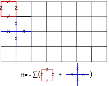
2 Exactly solvable models 16 2.1 XYZ-plaquette models . . . 18
2.1.1 Code subspace . . . 19
2.1.2 Low-energy excitation . . . 22
2.1.3 Duality . . . 24
2.2 No-string rule . . . 28
2.3 3D local qupit code . . . 29
2.3.1 Sufficient condition for the no-string rule . . . 32
2.3.2 Logical operators . . . 39
3 Technical tools for studying generic quantum many-body systems 43 3.1 Operator extension of strong subadditivity of entropy . . . 44
3.1.1 Proof of Theorem 5 . . . 45
3.2.1 Application to the finite-temperature systems . . . 49
3.2.2 Quasi-adiabatic continuation . . . 50
3.3 Deformation moves . . . 52
3.4 Regularization of the entanglement Hamiltonian . . . 56
4 Long-range entanglement is necessary for a topological storage of quantum infor-mation 60 4.1 1D system : correlation decay limits topological protection . . . 63
4.2 2D system : an inequality between topological entanglement entropy and topological degeneracy . . . 64
4.3 Higher-dimensional systems . . . 69
4.4 Bounds for more generic systems . . . 69
4.5 Stability of the lower bound . . . 70
5 Structure of the entanglement Hamiltonian 72 5.1 Approximately conditionally independent states . . . 73
5.2 Correlation bound for the entanglement Hamiltonian . . . 74
5.2.1 Modified form of exponential clustering theorem . . . 75
5.2.2 Derivation of the correlation bound . . . 76
5.3 Physical interpretation . . . 77
6 Perturbative analysis of topological entanglement entropy 79 6.1 The setup . . . 80
6.2 Deformation move for ac0-bounded states . . . 81
6.3 Ground state of exactly solvable models . . . 84
6.4 Higher-dimensional deformation move . . . 86
6.5 Stabilizer models at finite-temperature . . . 86
6.6 Higher order terms . . . 89
A Special quantum channels in quantum statistical mechanics 93 A.1 Construction of quantum channels from positive definite functions . . . 95
List of Figures
2.1 Kitaev’s toric code . . . 16
2.2 Defects can be created in pair, diffuse, and recombine to produce a logical operator. The energy barrier for this process is constant. . . 17
2.3 The vertex figure and the unit cell of our model. Qubits reside on the vertices. One can see thatBx px meets with anotherB x px at one vertex, whereas it meets withB y py and Bz pz at two vertices. . . 18
2.4 Arrangement of the stabilizer generators. The translation of unit cells form a tessellation. 19 2.5 Representation of the nontrivial constraints between the stabilizer operators. One can see that the multiplication of all the plaquette operators on a noncontractible closed surface reduces to the identity. At each vertices, there are either 1) exactly one X, one Y, and one Z or 2) twoXs and twoZs. . . 20
2.6 There is one surface operator and one string operator for each qubits. The surface operator corresponds to the product ofZZZZonY-plaquettes. The string operator is the line perpendicular to this surface, with a sequence that goes asY ZY XY ZY X· · ·. 22
2.7 A representation of a particle penetrating through a string-like excitation. The trun-cated surface operator is a product ofZ-plaquettes. The trajectory of the particle is the nontrivial support of the colored plaquette operators, which meets with theZ-surface at a point. . . 23
2.8 A stabilizer generator before enforcing any assumption . . . 29
2.9 A stabilizer generator after enforcing the commutation relation at the vertices. . . 30
2.10 Stabilizer group generators forCSαβγδ andCAαβγδ. . . 30
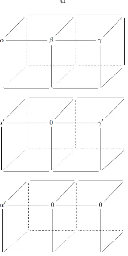
2.11 This diagram represents a deformation procedure. One can multiply a suitable choice of stabilizer elements so that the action of the string operator onB is 0 = (0,0). If two symplectic pairs on the diagonal line are linearly independent to each other, one can further deformC0 into 0. Repeat this procedure until we get rid of the entire line. . . 41
2.13 Two different kinds of boundary constraints. A and B are the unknown symplectic pairs and the cubes represent the stabilizer generators that share the support with the
logical operator only at these two sites. . . 42
2.14 Notation for the basis vectors . . . 42
2.15 Construction of the logical operators on a plane. Each of them can be mapped into each other by a unit translation. . . 42
3.1 Isolation move . . . 54
3.2 Separation move . . . 55
3.3 Absorption move . . . 55
4.1 1D chain with an open and closed boundary condition. . . 64
4.2 An example of the subsystem partition. . . 66
5.1 Levin-Wen configuration . . . 76
6.1 The shaded region represents an effect of the perturbation that is smeared out in space. We shall approximate this effect by a strictly local operator with a finite radiusR. The correction decreases superpolynomially withR. . . 81
6.2 Isolation move for ac0-bounded state . . . 82
6.3 Separation move for ac0-bounded state . . . 83
6.4 Absorption move for ac0-bounded state . . . 83
6.5 Subsystems involved in the calculation of the topological entanglement entropy. . . . 87
6.6 Deformed subsystems after applying the isolation move. . . 88
6.7 We have numerically computed I(A:C|B) and |TrCρABCHˆA:C|B|1 for 106 randomly generated mixed states. The largest observed ratio|TrCρABCHˆA:C|B|1/I(A:C|B) was 1.08. . . 90 6.8 We have numerically computed I(A:C|B) and |TrCρABCHˆA:C|B|1 for 106 randomly
Chapter 1
Introduction and preliminary
materials
In this thesis, we shall study the generic properties of gapped quantum many-body systems by (i) constructing exactly solvable models and (ii) exploiting the tools from quantum information theory. In fact, we shall restrict our focus to a set of quantum many-body systems described by a local Hamiltonian. We say a Hamiltonian H is local if it can be described by a sum of geometrically local terms with a bounded norm. Note that, while each of the geometrically local terms in the Hamiltonian have bounded norms,H itself might have an unbounded norm for an infinite system. Two HamiltoniansHandH0are typically labelled to bein the same phaseif they can be adiabatically connected to each other without closing the energy gap between the ground state and the rest of the spectrum.
One of the subtleties in defining a quantum phase lies on the fact that we are implicitly assuming an infinite volume limit of some sequence of Hamiltonians. After all, any generic finite dimensional Hamiltonian always has a gap between the first excited state and the ground state. Furthermore, as shown by Wen[1], there can be systems that have degenerate ground states in the thermody-namic limit even without any symmetry. Nowadays this is known as the topological ground state degeneracy.[1, 2, 3] The topological ground state degeneracy arises because an energy splitting be-tween the different “ground state sectors” are suppressed exponentially in the system size. Hence, the energy splitting for a finite system may be nonzero due to the finite-size effect.
One of the approaches for understanding these phases is to study their trial wavefunctions. For example, Laughlin was able to construct a wavefunction that predicted the partially filled Landau level of a quantum Hall system as well as the existence of a quasi-particle with a fractional charge.[7] Laughlin’s approach was subsequently vindicated by the discovery of an adiabatic path that in-terpolates between Laughlin’s wavefunction and a realistic system with a Coulomb interaction.[8] Also, Moore and Read proposed a trial wavefunction for aν= 52 fractional quantum Hall state, and predicted the existence of a quasi-particle that exhibits a non-Abelian statistics.[9]
Meanwhile, interesting developments were being made by several authors for the studies of one-dimensional quantum many-body systems. Partly inspired by Wilson’s idea of the renormalization-group (RG) flow,[10, 11, 12] White introduced a powerful numerical tool known as the density matrix renormalization-group (DMRG).[13] Around the same time, Fannes et al. introduced a class of quantum states known as the finitely correlated states (FCS).[14] It eventually became clear that DMRG and FCS have an intimate connection. Several authors have studied the so called matrix product state (MPS) formalism, and such an approach was successfully used in understanding the structure of 1D gapped systems.[15, 16, 17, 18, 19] A justification for using the MPS formalism in such setting is based on the area law of 1D gapped system.[20] The area law states that the entanglement entropyS(A) =−Tr(ρAlogρA) of a subsystemA is bounded by the size of its area,
as opposed to its volume. Hastings proved that this is the case for 1D gapped systems, and also showed that such states admit an efficient MPS description.[20]
The success of the MPS formalism was subsequently followed by the discovery other variational ansatzes, such as the projected entangled-pair states (PEPS)[21] and the multiscale entanglement renormalization ansatz(MERA)[22]. The motivation for studying these variational states are mainly twofold. First, by having a succinct description of the quantum many-body wavefunction, one can simulate their ground state properties efficiently. Second, one might be able to understand the generic structures that arise from these variational classes.
These variational states typically have a well-defined parent Hamiltonian.[23, 24, 25] If the parent Hamiltonian has a simple structure, it can substantially reduce the complexity of studying the properties of the quasi-particles. In particular, if the Hamiltonian consists of a sum of commuting terms, the underlying model is called as an exactly solvable model. Examples include the quantum double model and the string-net model.[3, 26]1 While it is hard to construct a physical system that
realizes such a Hamiltonian exactly, the virtue of these models is that the properties of the phase are stable against a small enough perturbation.[28, 29, 30] For example, consider the toric code.[3] As noted by Kitaev,[3] a perturbation theory calculation of the ground state degeneracy splitting decays exponentially in the system size. Recently, this result was put on a rigorous ground by several authors.[28, 29, 30, 31] Once such a stability bound is obtained, one can formally use the
quasi-adiabatic continuation technique to obtain rigorous statements about the properties of the phase.[32, 33]
For example, a rather obvious consequence of the gap stability is the stability of the particle statistics and the logical operator that can map one of the ground states to another.[29] Under the adiabatic evolution, the quasi-particle excitations may spread out to a length that is comparable to its correlation length. Hence, the conventional braiding operation can be still described by a dressed string-like operator. Higher-dimensional analogues of these statements can be obtained quite straightforwardly. An important lesson that one can learn from these examples is that, once we are given a model with a protected energy gap, important properties of its phase can be rigorously proven to be stable under a generic perturbation that is sufficiently weak. Therefore, one can consider these exactly solvable models as representatives of each gapped quantum phases.2
For these exactly solvable models, there is a general tradeoff bound that constrains a number of topologically protected ground states and its ability to protect against creation and diffusion of the quasi-particles.[34, 35, 36, 37, 38] When applied to two-dimensional systems, these tradeoff bounds imply that there has to be a constant energy barrier to construct a map from one of the degenerate ground states to another ground state. Recall that Arrhenius’ law states that a transition rate for such processes is of the order e−β∆E, where β is the inverse temperature and ∆E is the energy barrier. Since this expression alone does not account for the entropic contributions, it must not be considered as a mathematically rigorous result. However, this expression does cast doubt in using two-dimensional topologically ordered systems as a stable quantum memory without any active intervention. Indeed, there is a rigorous upper bound on the decoherence time for Kitaev’s toric code that is independent of the system size.[39]
On the other hand, it is well-known that a variant of the toric code in four spatial dimensions can have an extensive energy barrier that grows with the system size.[40] Later Alicki et al. were able to obtain a rigorous lower bound on the decoherence time that scales exponentially with the system size.[41] An important open question was whether it is possible to have such a stable quantum memory in three spatial dimensions. A number of authors have introduced a possible generalization of two-dimensional exactly solvable models to three spatial dimensions, but they were all shown to have a constant energy barrier.[42, 43, 44, 45] Later we have obtained yet another variant of these models, which was motivated from the fact that the previously known models could be manifestly decomposed into the “electric” and the “magnetic” part, so that at least one of them has a constant energy barrier.[46] This new model did not have such a manifest decomposition, yet it shared all the qualitative features of the three-dimensional (3D) toric code.
Soon it was realized by Yoshida that there is a good reason behind why such conclusion was 2However, it is not clear if one can always obtain such exactly solvable models foranytopologically ordered phase.
inevitable.[47] He showed that, given a three-dimensional system described by a stabilizer group formalism with a bounded number of encoded qubits, the energy barrier is always bounded by a constant. Roughly at the same time, Haah published his breakthrough result which seemed to have many counterintuitive properties.[48] One of the defining properties of Haah’s model is that the quasi-particles cannot move freely without paying an extensive energy cost that grows with the length it travels.[49] Due to this reason, his model quickly became a candidate for a self-correcting quantum memory in 3D. However, it was later realized that the decoherence time only grows as O(eβ2).[50] This bound does not grow with the size of the system, so Haah’s model is not a self-correcting quantum memory in a strict sense. Nevertheless, it is interesting to see that one can have a substantially longer lifetime than ordinary two-dimensional quantum memories at a low temperature. The first part of the thesis will be about the results that hinge on these developments. More specifically, we will describe two exactly solvable models that are similar to (i) the 3D toric code and (ii) Haah’s model. These shall be covered in Chapter 3.
The direction of the rest of the thesis shall be rather different in that we will be studying the
generic propertiesof a gapped quantum many-body system from a rather small set of assumptions. More specifically, we shall assume that (i) the system is gapped and (ii) it satisfies a certain form of an area law. It is widely believed that the area law is true for a gapped quantum many-body system, but there are several reasons to be careful about such an assertion. For one thing, the area law has been only established for one-dimensional systems.[20, 51, 52, 53] Unfortunately, the techniques used in these works do not seem to have an easy generalization that is applicable to higher dimensional systems. Also, Michalakis was able to obtain a rigorous bound on the change of the entanglement entropy under an adiabatic evolution.[54] In this stability bound, a logarithmic divergence is present in any systems that are supported on ad≥2-dimensional lattice. These results suggest that, even if area law is true, rigorously proving it ind≥2 spatial dimensions is likely to be a difficult task.
Therefore, instead of attempting to prove the area law, we shall take it as an axiom and study its consequences. The key idea lies on an observation that (i) there is a special structure that arises for states that are conditionally independent and (ii) the RG fixed-point ground state wavefunction of a topologically ordered system has many subsystems with such a property.[55] These observations shall be later explained in more detail, but for the moment we would like to sketch the general principle behind this approach. A tripartite stateρABC isconditionally independentif its conditional mutual
informationI(A:C|B) =S(AB)+S(BC)−S(B)−S(ABC) is equal to 0. If the state is conditionally independent, there are several different ways to reconstruct the global state ρABC from the local
reduced density matrices, such asρAB andρBC. There are several scenarios in which this property
can be exploited.
For example, suppose we are given two quantum states, say |ψ1iand|ψ2ithat are topologically
restricted to their local subsystems. The local indistinguishability would imply that the local reduced density of these two states are identical. At least in this idealized setting, one can conclude that the conditional mutual informationI(A:C|B) for the two states cannot be equal to 0. Otherwise, one would be able to reconstruct the global state from the local reduced density matrices.[55] Since the local reduced density matrices were assumed to be identical, the reconstructed states for |ψ1iand
|ψ2imust be identical to each other. However, such result contradicts the original assumption: that
|ψ1iand|ψ2iare orthogonal to each other.
The preceding argument is one of the many implications of the conditional independence. On one hand, this is encouraging in that we can obtain strong statements about quantum states without resorting to the properties of its parent Hamiltonian. On the other hand, a more careful analysis must be worked out. For example, a big open question in quantum information theory concerns a structure of states that are approximately conditionally independent. Realistic quantum states that arise as a ground state of a quantum many-body system will generically have a small conditional mutual information, rather than saturating its minimal value exactly. Hence, statements that are robust against such small deviation of the conditional independence condition is highly desirable.
An important tool that shall be used in conjunction with the preceding idea is the quasi-adiabatic continuation.[33, 56, 57, 58, 59, 60, 61, 29] Quasi-adiabatic continuation asserts that, given a set of approximately degenerate ground states |ψi(s)ii=1,···N that are sufficiently separated from the rest
of the spectrum by a constant along an adiabatic path s ∈[0,1], there exists a unitary operation U(s) such that
N X
i=1
|ψi(s)i hψi(s)|=U(s) N X
i=1
|ψii hψi|U(s)† (1.1)
for alls∈[0,1]. Further, the unitary operator U(s) is generated by a sum of path-dependent quasi-local generators with a superpolynomially decaying tail. A similar statement can be obtained even if the system only preserves the bulkmobilitygap alone, see Ref.[61].
1.0.1
How to read this thesis
Due to the scope of the thesis, we explain the necessary background materials to read each of the chapters. Chapter 2 concerns exactly solvable models that can be described by the stabilizer group formalism, which is briefly explained in Section 1.2. Therefore, the technical tools used in Chapter 3 will be irrelevant for the discussion. On the other hand, Chapter 4–6 will be based on the tools described in Chapter 3. In Chapter 4, we shall construct a set of inequalities between long-range entanglement and a topological ground state degeneracy. This result is based on the strong subadditivity of entropy alone, which is explained in Section 1.1. Chapter 5 studies a structure of the entanglement Hamiltonian in gapped quantum many-body systems. For this work, one would need Section 3.1,3.3, and 3.4. In Chapter 6, we establish a first-order perturbative stability of the topological entanglement entropy. All of the technical tools in Chapter 3 will be needed to understand the material. In Appendix A, we describe some of the technical tools that were developed in an attempt to attack the problems discussed in this thesis. These tools were superseded by the tools described in the main text of the thesis. Nevertheless, we list these results since they may be interesting in their own right.
1.1
Ground state properties of a topologically ordered
sys-tem
In this section, we review some of the well-known facts about topologically ordered systems, mainly focusing on its ground state properties. Of course, it is not clear if the ground state wavefunction alone gives a sufficient information to completely determine its underlying phase. This is due to the fact that the properties of its quasi-particles may not be completely determined by the ground state wavefunction alone. For example, there exists a gaplessHamiltonian whose ground state subspace is exactly equal to that of the toric code Hamiltonian.[72] Such an example shows that one must impose a certain “naturalness” condition to discuss the properties of the quasi-particles. However, the situation may not be so bad in light of the result by Zhang et al.[73] They have shown that one can infer the elements of the topologicalS-matrix andU-matrix from the ground state entanglement alone. For certain systems, these data are sufficient to determine all the important properties of the topological phase, see Ref.[74].
1.1.1
Topological ground state degeneracy
behavior for a fractional quantum Hall system.[2] The character of such a degeneracy is different from the degeneracy that arises from a symmetry breaking phenomenon. For example, consider an Ising model at zero temperature. The degenerate ground states can be distinguished by a local observable, namely theσzoperator. This is not the case for a topologically ordered system. No local
observable can distinguish different ground state sectors. The local indistinguishability property is at the heart of the topological protection of quantum information. In order to disturb the quantum information that is encoded in the ground state subspace, a highly nonlocal operation must be carried out. Furthermore, under a generic condition that is believed to be satisfied by many systems, the degeneracy is protected by any local perturbation that is sufficiently weak.[28, 29, 31] We note in passing that there are other types of topologically protected degeneracy that may arise.[3, 75, 76, 77, 78] We believe our tool can be applied to these systems as well, but we leave that for the future work.
1.1.2
Topological entanglement entropy
It was first discovered by Hamma et al. for Kitaev’s toric code model[79] and later generalized by Kitaev and Preskill[27] and Levin and Wen[71] that there exists a universal constant subcorrection term of the entanglement entropy that characterizes the phase. More precisely, given a simply connected subsystemA, its entanglement entropyS(A) can be expressed as
S(A) =a|∂A| −γ+O(e−|∂A|/ξ), (1.2)
whereais a nonuniversal constant,|∂A|is the boundary area ofA,γis the topological entanglement entropy, andξ is the correlation length of the system. It was argued by these authors thatγ is an invariant, in that its value changes very little under an adiabatic evolution of the system that does not close the bulk gap. While a substantial amount of numerical work has confirmed their predictions,[80, 81, 74, 82] rigorously proving its stability still remains as an open problem. In fact, Bravyi has an unpublished model which can be adiabatically connected from a trivial state, yet has a nonzero amount of topological entanglement entropy defined as in Ref.[27, 71, 83].[83] Bravyi’s counterexample shows that a constant subcorrection term of the entanglement entropies in such systems is not a stable invariant characterizing the phase. But then, what does γ represent? The numerical examples give values that are close to what the ideal wavefunctions predict.[80, 81, 74, 82] Hence, it is natural to conclude that there exists an alternative definition of the topological entanglement entropy that evades Bravyi’s counterexample.
alone. Since the quasi-particles in two spatial dimensions can be used to perform a fault-tolerant quantum computation,[3] it is important to have a correct definition of the ground state observables to characterize such phases from the microscopic Hamiltonian. We do not have a complete answer to this problem, but we shall propose an alternative definition that are in many ways natural. More specifically, we shall derive a universal inequality relating the number of topologically protected states and a certain linear combination of the entanglement entropies. This linear combination is reduced to the topological entanglement entropy for an idealized wavefunction that is a fixed-point of some RG flow. Furthermore, the inequality is saturated with an equality for Abelian anyon models, giving an automatic one-sided stability bound for this newly defined quantity. Of course, the one-sided stability result does not imply the stability of the topological entanglement entropy. Nevertheless, our result implies that it suffices to prove a rigorous upper bound for the topological entanglement entropy in order to prove its stability under an adiabatic evolution.
After the discovery of the topological entanglement entropy, several authors have attempted to find its finite-temperature generalizations. For a two-dimensional system, it was quickly realized that the topological entanglement entropy vanishes at any finite temperature.[85, 86] On the other hand, the topological entanglement entropy does survive at finite temperature for certain systems, see Ref.[43, 87]. There are some subtleties that are worth mentioning. For a three-dimensional variant of the toric code, there exists an order parameter that is analogous to the topological entanglement entropy.[85] The value of the order parameter vanishes at a sufficiently high temperature, but it attains a nonzero value even in the thermodynamic limit below a certain critical temperature. On the other hand, Hastings showed that the model can be mapped to a thermal state of a classical Hamiltonian under a finite-depth local quantum circuit.[88] These two results together imply that the topological entanglement entropy can be of a classical origin at a finite temperature. Therefore, it is not clear if it is a stable invariant under a small perturbation. We make a partial progress in showing the perturbative stability of this quantity. A similar technique shall be used to prove a first-order perturbative stability of the ground state topological entanglement entropy as well.
1.1.3
Entanglement Hamiltonian
theory(CFT) that describes the FQHE wavefunction.3
Since the discovery of Li and Haldane, a number of authors followed up by investigating different variational states.[90, 91, 92, 93, 94, 95] One of the conclusions uniformly drawn from these works is that the spectrum of the entanglement Hamiltonian can be described by the spectrum of some local Hamiltonian. Further, this spectrum contains information about the phase. Unfortunately, such emergent local structure of the entanglement Hamiltonian was studied only by either investigating a class of variational states[95, 94] or performing numerical experiments.[90, 91, 92, 93]
In Chapter 5, we make a partial progress in understanding this local structure. More specifically, we shall show that a judiciously chosen linear combination of the entanglement Hamiltonian has a small correlation with almost all local observables, given that the ground state wavefunction obeys a certain form of an area law. Our result shows that the local structure of the entanglement Hamiltonian may be attributed to the area law of entanglement entropy[96] and the exponential clustering theorem[56, 57], which are believed to be the generic properties of a gapped quantum many-body system.
1.2
Information measures
A fundamental quantity in quantum information theory is the von Neumann entropyS(ρ). Definition 1.
S(ρ) :=−Tr(ρlogρ). (1.3)
The von Neumann entropy quantifies the amount of information that is present in a sequence of many copies of the state. Schumacher showed thatρ⊗n can be compressed inton(S(ρ)−δ) qubits with an error that vanishes inn→ ∞limit for any nonzero δ.[97]
Entanglement entropy is a canonical measure for quantifying entanglement in a bipartite system. Given a quantum stateρ, its entanglement entropy of a subsystemAis defined as follows.
Definition 2.
S(A) :=−Tr(ρAlogρA), (1.4)
whereρA is the reduced density matrix over the subsystemA.
Given a multipartite system, one can define a linear combination of the entanglement entropy. For example, mutual information is a measure of correlation that is present between two subsystems. 3In the literature, the spectrum of the entanglement Hamiltonian is called as theentanglement spectrum. We
Definition 3. A mutual information between two subsystemsA andB is
I(A:B) =S(A) +S(B)−S(AB). (1.5)
This also has an operational meaning, see Ref.[98]. We also define conditional mutual informa-tion.
Definition 4. A conditional mutual information betweenA andC with respect toB is
I(A:C|B) =S(AB) +S(BC)−S(B)−S(ABC). (1.6)
The conditional mutual information has an operational meaning in the context of a quantum state redistribution protocol, see Ref.[99]. We also define a quantum relative entropy, which is a quantum analogue of the Kullback-Leibler divergence.
Definition 5. A relative entropy D(ρkσ)between two quantum statesρandσis the following.
D(ρkσ) :=Tr(ρ(logρ−logσ)). (1.7)
The relative entropy appears in the context of quantum hypothesis testing, see Ref.[100, 101, 102, 103]. Another standard distance measure between quantum states is the Schatten p-norm. Given an operatorO, itsp-norm is defined as follows.
Definition 6.
|O|p:= ( X
i
epi)1/p, (1.8)
where{ei}is a set of eigenvalues of |O|:= (O†O)
1 2.
A special attention must be given top= 1 andp=∞case. In particular, the Schatten∞-norm is typically called as theoperator norm. We shall denote such norm as follows:
kOk=|O|∞. (1.9)
1.2.1
Inequalities
A linear inequality is an inequality that is linear in the von Neumann entropy and quantum relative entropy. One of the most basic linear inequalities is the concavity of the von Neumann entropy, which easily follows from the operator convexity of a functionf(x) =xlogx.[104]4
The concavity of the von Neumann entropy implies the nonnegativity of the quantum relative entropy D(ρkσ) := Tr(ρ(logρ−logσ)) between two quantum states ρand σ. This can be easily seen by dividing the both sides of Equation 1.10 byc and taking thec→0+ limit.
There exists a class of inequalities that cannot be directly derived from the concavity of the von Neumann entropy. These are the descendants of the joint convexity of the quantum relative entropy:
cD(ρ1kσ1) + (1−c)D(ρ2kσ2)≥D(cρ1+ (1−c)ρ2kcσ1+ (1−c)σ2), c∈[0,1], (1.11)
whereρ1, ρ2, σ1, σ2are some density matrices.[105] Equation 1.11 implies one of the most important
results in quantum information theory, which is known as the monotonicity of the quantum relative entropy. The monotonicity of the quantum relative entropy asserts that the relative entropy between two quantum states does not increase under a quantum channel. That is,
D(ρkσ)≥D(Φ(ρ)kΦ(σ)) (1.12)
for a completely positive trace-preserving map Φ.
A rather straightforward consequence of Equation 1.12 is the strong subadditivity of entropy(SSA), which asserts that the conditional mutual information is nonnegative:
I(A:C|B)≥0. (1.13)
Another useful inequality for the purpose of this thesis is Fannes’ inequality, which holds for any density matricesρandσ:
|S(ρ)−S(σ)| ≤2logd−2log 2, (1.14)
where=1
2|ρ−σ|1.[106] We note in passing that an optimal improvement of the Fannes’ inequality
was recently obtained by Audenaeart:
|S(ρ)−S(σ)| ≤logd+H(,1−), (1.15)
whereH(p,1−p) is a binary entropy.[102]
H(p,1−p) =−plogp−(1−p) log(1−p). (1.16)
1.3
Quantum error-correcting code
Definition 7. [107] A quantum code C detects an error E ∈ B(H) if there exists a constant c(E)
such that
∀ |ψ1i,|ψ2i ∈ C,hψ1|E|ψ2i=c(E)hψ1| |ψ2i. (1.17)
The vectors of the quantum code shall be called as thecodewords. The physical systems that are described by the quantum code typically consist of particles with bounded dimensions, say d. For such systems, there always exists a canonical basis forB(H) that is described by the operators in a tensor product form:
∀O∈ B(H), O= X
i1,···,in
ai1,···inUi1⊗ · · · ⊗Uin, (1.18)
whereUin is an operator supported on thelocal Hilbert spacedescribing thenth particle.[108]
Fur-thermore,{Ui}i=1,···,d2can be chosen to be a complete set of unitary operators that are orthonormal.
Tr(UiUj†) =dδij. (1.19)
The operators do not necessarily have to be unitary, but it is a convenient choice for many of the analysis. Ford= 2 case, one can actually get more structure: the basis set for the operators can be chosen to be Hermitian as well as unitary. The elements of this set is known as the Pauli operators:
I= 1 0 0 1
, X :=σx=
0 1 1 0
, Y :=σy =
0 i
−i 0
, Z:=σz=
1 0
0 −1
. (1.20)
Generally speaking, an operator of the tensor product form shall be called as aweight-woperator if wof the local operators are not the identity operator. Thecode distance of a quantum code is the minimal weight of the operator which is not detectable.
If the system is subject to an interaction with its environment, the underlying physical process can be modeled by a quantum channelE, see Ref.[109]. It is typically convenient to use aKraus representationof a quantum channel{Ej}:
E(O) =X
j
EjOEj†. (1.21)
One can formally define what it means for a quantum code to be able to correct errors from such processes.
Definition 8. A quantum code C corrects errors fromE if
P Ei†EjP =αijP (1.22)
operators ofE.
An interesting class of quantum error-correcting code is the so calledtopologically ordered systems. Formally, we define a topological quantum order as follows.
Definition 9. [59] A set of orthonormal states {|ψii}i=1,···,N satisfies a (r, )-TQO condition if
they satisfy the following inequalities:
| hψi|O|ψii − hψj|O|ψji | ≤ kOk
| hψi|O|ψji | ≤2kOk, (1.23)
whereO is a bounded operator that can be supported on a ball of radiusr.
Ifis set to 0, the TQO-(r, ) condition implies that the quantum code spanned by{|ψii}i=1,···,N
can detect any error that is supported on a ball of radius r. We note in passing that the code distance d and the TQO-radius r are not equal to each other in general. More specifically, their relation depends on the dimensionality of the underlying lattice. For example, consider Kitaev’s toric code.[3] The code distance on a L×L lattice is L. On the other hand, the code satisfies a TQO-([L2]−1,0) condition. On the other hand, a 4D generalization of the toric code (i) has a code distance that grows as Θ(L2) but (ii) satisfies the TQO condition with the TQO-radiusr=O(L).[40]
1.3.1
Stabilizer codes
An important class of quantum error-correcting code is the stabilizer code, which was first introduced by Gottesman.[110] One of the advantages of the stabilizer code is that it has an efficient description of the codewords in terms of a set of commuting operators. The quantum code can be described by a set of n−k commuting operators, wheren is the number of qudits and k is the number of encoded qudits. More specifically, the code is a set of states that are simultaneous +1 eigenstates of thestabilizer groupelements.
The stabilizer group is defined as an Abelian subgroup of the Pauli group which does not contain
with a prime dimension.5 The unitary generalizations of theX andZoperators are given as follows:
Xij= 1 j=i+ 1 modd (1.24)
= 0 otherwise. (1.25)
Zij=ωi j=i (1.26)
= 0 otherwise, (1.27)
whereωis thedth root of unity. We shall denoteXα1Zα2 asS
αwith asymplectic pairα= (α1, α2).
As in the binary code case,X andZ satisfies a nontrivial commutation relation.
XZ=ZXω. (1.28)
We define a symplectic product:
hα, βi=α1β2−α2β1. (1.29)
The symplectic product has two useful properties. First, a commutation relation of two generalized Pauli operators can be determined from a symplectic product of the symplectic pairs describing each of the generalized Pauli operators.
SαSβ =SβSαωhα,βi, (1.30)
Second, in prime dimensions, a symplectic product of two symplectic pairs is 0 if and only if they are equivalent to each other up to a constant factor.
Lemma 1. Ifα6= (0,0), andda prime number,
hα, βi= 0 (1.31)
if and only if β=aα for somea∈Zd.
For abinary stabilizer code, one can measure thesyndromeof the code by measuring the stabilizer group elements. If the error rate is sufficiently low, one can make an intelligent guess on where the errors occurred by measuring these operations.[40] Alternatively, one can engineer a Hamiltonian whose ground state subspace is the code subspace of the stabilizer code:
H =−X i
si, (1.32)
5The generalization can be straightforwardly carried out for any dimensions, but there are some subtleties that
where si is the generator of the stabilizer group. Of course, this construction works only if si is
Hermitian.
For a general qudit stabilizer code, one should hermitize the stabilizer generators in order to engineer a Hamiltonian whose ground state subspace is described by the code. Ifdis an odd prime number,
Pα(r) =
1 d
d−1
X
m=0
(ωrSα)m (1.33)
is a complete set of orthogonal projections.[108] Therefore, a simultaneous +1 eigenstate of the following projector becomes the codeword of a qudit stabilizer code:
Ps,r=
1 d
d−1
X
m=0
smωrm, (1.34)
Chapter 2
Exactly solvable models
One of the simplest topologically ordered systems is Kitaev’s toric code.[3] Consider a square lattice, where the qubits lie on the edges of the graph. Toric code can be formally defined as a set of degenerate ground states of the following Hamiltonian:
H =−X s
As− X
p
Bp, (2.1)
where As is the “star” operator and Bp is the “plaquette” operator. A star operator on a site s
is defined to be a tensor product ofX operators along the edges that are touchings. Similarly, a plaquette operator on a plaquettepis defined to be a tensor product ofZ operators along the edges surrounding the plaquette. By the construction, one can easily see that all of the terms commute with each other. There are other properties of this system that can be easily verified, such as the braiding statistics and the ground state degeneracy, see Ref.[3].
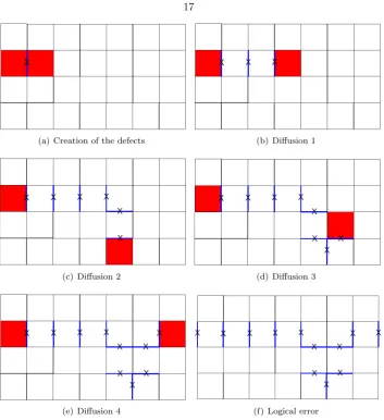
[image:25.595.237.414.538.678.2]While the toric code can reliably store a quantum information at zero temperature against a generic perturbation,[28, 29] it fails to do so at finite temperature.[39] This is due to the fact that it only takes a constant energy barrier to produce a logical operator, see FIG.2.2
(a) Creation of the defects (b) Diffusion 1
(c) Diffusion 2 (d) Diffusion 3
[image:26.595.150.504.53.440.2](e) Diffusion 4 (f) Logical error
Figure 2.2: Defects can be created in pair, diffuse, and recombine to produce a logical operator. The energy barrier for this process is constant.
There is a straightforward generalization of the toric code to a three-dimensional system. This model is typically known as the three-dimensional (3D) toric code. Analogous to the construction of the toric code, 3D toric code is defined to be a set of degenerate ground states of the following Hamiltonian:
H =−X s
As− X
p
Bp, (2.2)
where As and Bp are defined similarly to the 2D toric code. More precisely, qubits reside on the
edges of a cubic lattice. As is a tensor product of theσx operators meeting with a sites. Bp is a
tensor product of σz operators surrounding a plaquette p. There is a general intuition that as the
information encoded in the ground state cannot be protected against a phase flip error. An easy way to see this is to consider a sequence of σz operators that makes a noncontractible loop. Once
the defects are created, they can diffuse freely without paying any extra energy cost. There are other models that have similar properties to the 3D toric code, in that their Hamiltonian can be manifestly divided into two parts. One part is analogous to the star operators, responsible for the protection against the phase flip error. The other part is responsible for the protection against the bit flip error. Section 2.1 provides a model that evades such a natural decomposition. However, the conclusion is that these models also have a finite energy barrier.
2.1
XYZ-plaquette models
We place qubits on vertices of a 4-valent 3D lattice. The stabilizer group is generated by the following operators:
Bxp = Πi∈pXi (2.3)
Bpy= Πi∈pYi (2.4)
Bpz= Πi∈pZi, (2.5)
wherepis the plaquette and{i∈p}denotes a set of vertices on a plaquettep. We shall partition a set of plaquettes intoPx(Py, Pz), which corresponds to a set of nontrivial supports forBpx(Bpy, Bpz).
We shall call elements of these sets asX−(Y−, Z−)plaquettes.
This model is inspired by the construction of the 3D topological color code.[42] For the topological color code, qubits reside on the vertices of a 3D lattice, and the lattice is 4-valent. The stabilizer generators are either a product ofXs or a product ofZs, and they correspond to the unit cells of different dimensions; in one example, generators are either in cubic form or plaquette form. Our approach differs from theirs in a sense that we only allow plaquette operators as stabilizer generators.
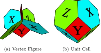
[image:27.595.238.413.551.643.2](a) Vertex Figure (b) Unit Cell
Figure 2.3: The vertex figure and the unit cell of our model. Qubits reside on the vertices. One can see thatBpxx meets with anotherBxpx at one vertex, whereas it meets withBypy andBpzz at two vertices.
6 plaquette operators that share a nontrivial support. Each plaquette operators meet with the same kind of plaquette operator on each vertices and meet with 4 other plaquette operators on 2 vertices. Thus the assignment in Figure 2.3(a) guarantees the commutativity between the stabilizer generators. We must point out that not every lattice structure allows vertex figures like Figure 2.3(a). There are only 4 translationally invariant convex tessellations that have tetrahedral vertex figure: bitruncated qubic honeycomb, cantitruncated cubic honeycomb, omnitruncated cubic honeycomb, and cantitruncated alternated cubic honeycomb.[112] Only the first three admits an arrangement of plaquette operators similar to Figure 2.3(a) at every vertex. Here we mainly study the bitruncated qubic honeycomb model for its simplicity, but analogous results shall be discussed in full generality if possible. The unit cell is shown in Figure 2.3(b) and its tessellation is shown in Figure 2.4. The bitruncated cubic honeycomb is a space-filling tessellation made up of truncated octahedra. It has 14 faces, 36 edges, and 24 vertices. There are 6 square faces and 8 hexagonal faces. Without loss of generality, one can set the 6 square faces to be theY plaquette operators, 4 of the hexagonal faces to be the X-plaquette operators, and the remaining hexagonal faces to be theZ-plaquette operators. Hamiltonian is a sum over these plaquette operators.
H=−J( X
px∈Px
Bpx
x+
X
py∈Py
Byp
y+
X
pz∈Pz
Bpz
[image:28.595.230.447.353.537.2]z). (2.6)
Figure 2.4: Arrangement of the stabilizer generators. The translation of unit cells form a tessellation.
2.1.1
Code subspace
Euler characteristicχis defined as an alternating sum ofkns, wherekndenotes a number of cells of
dimensionn.
χ=
d X
i=0
One of the main ideas that we used here is thatχcan be also written as an alternating sum of Betti numberbis.
χ=
d X
i=0
bi(−1)i (2.8)
biis the rank of then-th singular homotopy group. We briefly explain the Poincar´e duality. Although
it has different forms depending on the context, here we use the one originally introduced by Poincar´e himself.
Theorem 1. (Poincar´e, 1895) bk=bd−k for a closed orientable d-dimensional manifold.
A number of encoded qubits can be computed from the size of the stabilizer group and the number of physical qubits. Since the plaquette operators are not independent to each other, we must count the number of independent relations. In such a pursuit, a geometrical interpretation of our model becomes useful. Note that multiplying all the plaquette operators on a unit cell reduces to an identity, see Figure 2.3(b). Since any contractible closed surface on the lattice can be represented as a union of unit cells, one can see that a multiplication of the plaquette operators onany contractible closed surface reduces to the identity. Therefore we haveC−1 independent relations which generate smooth deformations, whereCis the number of unit cells. We must subtract 1 because multiplying all but one cell results in a relation for that very cell.
Let us consider a periodic boundary condition in all 3 directions. There exists a noncontractible surface that reduces to the identity as one can see in Figure 2.5(a) and Figure 2.5(b). Since there are 3 topologically distinct noncontractible surfaces, we have 3 independent relations, resulting inC+ 2 independent relations. Finally, multiplying allX-like operators adds one independent relation. One can check that multiplication ofYs and multiplication ofZs are implied by the previously mentioned relations.
[image:29.595.198.456.503.650.2](a) Top view (b) Side view
Accounting for these relations, the number of encoded qubits is V −F +C+ 3 = 3 under a periodic boundary condition, where V is the number of vertices, F is the number of faces, and C is the number of unit cells. The first two correspond to the number of qubits and the number of plaquette operators. The remaining terms represent a number of independent relations between plaquette operators. We shall show that the number of encoded qubits only depend on the second Betti number.
Lemma 2. For a stabilizer group{Bxpx, B
y py, B
z
pz}, the number of encoded qubits is b2.
Proof : Let us consider the dual lattice. This can be constructed by replacing thek-dimensional object to a (d−k)-dimensional object. For instance, a vertex of the dual lattice resides on the center of the unit cells of the original lattice. A face on the dual lattice can be constructed by connecting the edges so that the resulting surface is perpendicular to the edges of the original lattice. The Euler characteristic is trivially 0 due to the Poincar´e Duality. The unit cells of the resulting dual lattice is an irregular tetrahedron. Let us denotekis to be the number ofi-dimensional cells on the dual
lattice. The total number of vertices in the original lattice becomesk3, which is the number of unit
cells in the dual lattice. Similarly,F is identical tok1 andC is identical tok0. Note thatk2=k3,
since each cell contains 4 faces and each faces meet with two tetrahedral cells. Therefore, we have
V −(F−C) =k3−k1+k0 (2.9)
=−k3+k2−k1+k0= 0. (2.10)
Hence
k=V −(F−(C−1 + 1 +b2)) (2.11)
=b2, (2.12)
whereb2 is the second Betti number of the manifold. One can also use this intuition to prove that
the group generated by the plaquette operators does not contain−I. Lemma 3. hBx
px, B
y py, B
z
pzidoes not contain−I.
product in the following canonical form.
ΠpxB
x pxΠpyB
y pyΠpzB
z
pz. (2.13)
SinceXY Z=i, the product of plaquette operators on a unit cell is 1. Similarly, for the product of plaquette operators on a noncontractible surface described in Figure 2.5(a) and Figure 2.5(b), we have 4nvertices whereX, Y,andZ meet each other. Hence we arrive at the same conclusion. Since any product of the plaquette operators that results in a trivial operator can be constructed by these constraints, the group does not contain−I.
There are two logical operators that are reminiscent to the surface and the string operator of the 3D toric code. These are drawn in Figure 2.6. One can see the surface operator on the top of the lattice system, which is a product of Bz
pys on a layer of Y-plaquettes. The complementary
[image:31.595.251.389.380.523.2]logical operator is the string operator that has a sequence of Y ZY XY ZY XY ZY X· · · along the line perpendicular to the surface operator. This string winds around the torus and completes a noncontractible loop. These two operators anticommute with each other and both of them commute with the stabilizer generators. One can similarly define two sets of complementary operators in other
Figure 2.6: There is one surface operator and one string operator for each qubits. The surface operator corresponds to the product of ZZZZ on Y-plaquettes. The string operator is the line perpendicular to this surface, with a sequence that goes asY ZY XY ZY X· · ·.
directions. One can easily check the expected commutation and anticommutation relations.
2.1.2
Low-energy excitation
attains a nontrivial phase. In 3D, one can always contract the trajectory of the loop to a point, unless the loop winds around the torus. Hence, one needs higher dimensional objects to attain a nontrivial braiding statistics. In 3D, there are closed string-like excitations and particle-like excitations.[113, 43] When the particle winds around the string, the system attains a nontrivial phase.
Despite the fact that our model is made up of only plaquette operators, it shows a similar behavior. A pair of particle-like excitations can be created from the vacuum by a constant energy. If we truncate a string-like logical operator, excitations form at the end points. When the particle-antiparticle pair is created, they can diffuse without any extra energy cost. The closed string-like excitations can be similarly thought as a truncated surface-like logical operator. There are excitations near the boundary of the constraint. Therefore, the energy cost grows linearly with the size of the surface. If a particle penetrates the closed string, we find that
|ψInitiali=SP|Φi (2.14)
|ψF inali=U SP|Φi=− |ψInitiali, (2.15)
where S is the closed-string excitation, P is the particle excitation, and U is a trajectory of the particle. Therefore, the system picks up a phase ofeiπ in this process. This is illustrated in Figure
[image:32.595.248.393.448.544.2]2.7. One can see that as the particle penetrates through the surface operator and returns to the original position, it meets with the surface operator at one vertex, giving the anticommutation relation.
Figure 2.7: A representation of a particle penetrating through a string-like excitation. The truncated surface operator is a product ofZ-plaquettes. The trajectory of the particle is the nontrivial support of the colored plaquette operators, which meets with theZ-surface at a point.
boundary of the surface. Z-plaquettes trivially commute with the surface operator. X-plaquettes commute with the surface operator since they meet at two vertices. However, there areY-plaquettes meeting at exactly one vertex at the boundary. Hence we expect our system to be a stable classical memory.
2.1.3
Duality
Typically, a strong-weak duality relation relates a strong coupling limit of one model to a weak coupling limit of another model. We use a slightly different strategy here. We first show that our model can be mapped into an Ising gauge theory, from which we can use the Wegner-type duality relation with an Ising model.[114] Mapping from our model to the Ising gauge theory is not exact for a finite sized lattice, but this difference vanishes in the thermodynamic limit. Starting from the partition function of our model,
Z= Tr(exp(−βH)) (2.16)
= Tr(ΠSi∈S(coshβJ+SisinhβJ)), (2.17)
whereSi ∈ {Bpxx, B
y py, B
z pz},
Z = (coshβJ)ntr(Πi(1 +αSi)) (2.18)
= (coshβJ)ntr(
1
X
{ki}=0
ΠiαkiSiki). (2.19)
Note that there were two kinds of constraints: the constraints coming from the closed 2-manifold and the constraints coming from the space-filling products of X, Ys, and Zs. Therefore, we can write down the partition function in the following form:
Z = (2 coshβJ)n(X
c
αAc+ (1 +αnx)(1 +αny)(1 +αnz)−1 +C.T.). (2.20)
HereP
c is a sum over the configurations of the closed 2-manifolds. Ac is the number of plaquettes
for each configurations. C.T.corresponds to the cross terms between the closed 2-manifolds and the space-filling products of Xs, Ys, and Zs. nx,y,z corresponds to the number of X, Y, Z−plaquette
operators. The main idea is that the partition function is dominated by the first term in the thermodynamic limit. The cross terms can be written as
C.T.=X
c
αAc X
i∈{x,y,z}
αni−2nci, (2.21)
for a configurationc.
Lemma 4. There exists an0< 1,2<1such that
Ac+ni−2nci ≥1Ac+2ni (2.22)
for∀c, i.
Proof : Consideri=x. The left hand side of the inequality is
ncy+ncz−nxc +nx≥ncy+n c
z−(1−)n c
x+ (1−)nx (2.23)
≥(
2)Ac+ (1−)nx (2.24)
On the second line, we used the fact that the minimum is achieved forncy= 0.
ncz=ncx= 1
2Ac (2.25)
The same logic can be applied toi=z. Fori=y,
ncx+ncz−nxc +ny≥ncx+n c
z−(1−)n c
y+ (1−)ny (2.26)
≥(2 5 −
3
5(1−))Ac+ (1−)ny. (2.27) Similarly, we used the fact that the minimum is achieved if one of ncx or ncz is 0. Then we have a
2 : 3 ratio between the X−(Z−)plaquettes andY−plaquettes. Therefore, for > 1
3, we have such
(1, 2).
Lemma 5.
lim
vol→∞
Z(βJ) ZIG(βJ)
→1. (2.28)
, where ZIG(βJ) is a partition function for the Ising gauge theory with a temperature β and a
coupling constantJ. vol is the volume of the lattice.
Proof :
We use the following equation:
X
c
α1Ac =(2 coshβJ
0)n
(2 coshβJ0)n X
c
α0Ac (2.29)
= ( 1
2 coshβJ0)
nZ
IG(βJ0), (2.30)
where
Thus the cross terms can be bounded by
ZIG(βJ0)(
coshβJ coshβJ0)
nαδi2n, . (2.32)
whereδi= nni, where nis the total number of plaquettes. This expression becomes
ZIG(βJ0)((
1−t2
1−t21
)12t
2
δ1)n, (2.33)
where t = tanhβJ0. One can show that ( 1−t2
1−t
2
1
)12t
2
1δ < 1 for βJ > 0. Since the renormalized
coupling constantJ0is larger thanJ, these correction terms become negligible in the thermodynamic limit. Therefore,
| lim
vol→∞
Z(βJ)−ZIG(βJ)
ZIG(βJ)
| ≤ |ZIG(βJ
0)
ZIG(βJ)
λn+O(αn)|, (2.34)
whereJ0> J and 0< λ <1. Inn→ ∞limit, we get the desired result.
Lemma 6. Z−C.T.−(αnx+αny+αnz) =Z
IG(βJ), whereZIG is a partition function of the Ising
gauge theory on the same lattice with a temperature β and a coupling constantJ.
Proof : Consider a mapping Bx
px → ZZZZZZ, B
y
py → ZZZZ, B
z
pz → ZZZZZZ, where
Z· · ·Z are products ofZ on the edges of each plaquettes. The resulting model is an Ising gauge theory on a bitruncated cubic honeycomb. The partition function is
ZIG=tr(exp(−βH)) (2.35)
= (coshβJ)ntr(1 + tanhβJ Si), (2.36)
whereSis are eitherZZZZZZorZZZZdepending on the plaquette. Since the Pauli operators are
traceless, a product of the plaquette operators survives only if the union of the plaquettes form a union of closed manifolds.
ZIG(βJ) =Z−C.T.−(αnx+αny +αnz). (2.37)
Using the duality relation between the Ising gauge theory and the Ising model, we can map our model into an Ising model.
Proof:
Z = (coshβJ)ntr(Πi(1 + tanhβJ Si)) (2.38)
= (coshβJ)ntr(
1
X
{ki}=0
ΠiαkiSiki) (2.39)
= (2 coshβJ)n
1
X
{ki}=0
ΠiαkiΠeδ2(
X
j
kj;e), (2.40)
where Πe is a product over all the edges andPjkj;eis a sum overkjs that have nontrivial support
on an edge e. There are three such kjs. One can usekj;e= 12(1−ZZ), whereZZ is a product of
Zs on qubits that reside on the vertices of the dual lattice. For 8 spin configurations (Z1, Z2, Z3) =
(−1,−1,−1), (1,1,1), (1,−1,−1), (−1,1,−1), (−1,−1,1), (1,1,−1), (−1,1,1), (1,−1,1), they all satisfy the delta function. Furthermore, we have 2 combinations for (k1, k2, k3) = (0,0,0), 2
combi-nations for (0,1,1), (1,0,1), and (1,1,0). Plugging these relations in, we get
Z= (coshβJ)n
1
X
{Zi}=0
Πiα1−
1
2Zi+ ˆniZi−niˆ , (2.41)
where Zi±nˆi is theZ operator on the dual sites of the plaquettei. ˆni is the unit normal vector to
the plaquette. Therefore, up to a constant, the partition function is equal to the partition function of the Ising model with ˜βJ =−1
2ln tanhβJ.
Theorem 2. The XYZ-plaquette model with a coupling constant βJ is dual to the classical Ising model on a dual lattice with a dual coupling constant βJ˜ =−1
2ln tanhβJ.
Since the Ising model undergoes a finite temperature phase transition, so does our model. This is analogous to the behavior of the 3D toric code under a temperature change. As in our model, one can show that the 3D toric code has a critical temperature by using the duality relation with the Ising model. Below the critical temperature, there is a symmetry breaking with respect to a surface-like logical operator. The symmetry associated to the string-like logical operator is broken only at the ground state.
One important difference though, is that the 3D toric code can be decomposed into two classical Hamiltonians without spoiling the phase transition: the Hamiltonian responsible for correcting the bit flip error is identical to the Ising gauge theory, which has a finite temperature phase transition. On the other hand, the Hamiltonian responsible for correcting the phase flip error does not have a phase transition. Therefore, one can intuitively understand that the 3D toric code can only correct bit flip errors but not phase flip errors under the influence of a thermal bath. Our model does not allow such a decomposition. Once we get rid of any of the Bx
px, B
y py, or B
z
pz, the partition
temperature phase transition in 3D does not necessarily provide a self-correcting quantum memory.
2.2
No-string rule
One of the defining properties of Haah’s code is that it has no string-like logical operator.[48] Since we are dealing with a lattice system, one needs to precisely define what it means for an operator to be a string. Since this is an important concept, we first reiterate some of the definitions introduced by Haah.[48]
Definition 10. (Haah 2011) A set of sites{p1, p2,· · ·, pn} is a pathjoining p1 andpn if for each
pair (pi, pi+1)of consecutive sites there exists a stabilizer generators that acts nontrivially on their
pair simultaneously, for i= 1,· · · , n−1. A set M of sites is connectedif every pair of sites in M
are joined by a path inM. Aconnected Pauli operatoris a Pauli operator with connected support.
Definition 11. (Haah 2011) LetΩ1,Ω2be congruent cubes consisting ofw3 sites, andObe a finite
Pauli operator. A tripleη = (O,Ω1,Ω2)is a logical string segment if every stabilizer generator that
acts trivially on bothΩ1 andΩ2commutes with O. We call Ω1,2 the anchor. The directional vector
of η is the relative position of Ω1 toΩ2. The lengthis the l1-length of the directional vector, and
the width isw.
Definition 12. (Haah 2011) A logical string segment η = (O,Ω1,Ω2) is connectedif there exists
two sites p1 ∈ Ω1, p2,Ω2 that can be joined by a path in supp(O)∪ {p1, p2}, where supp(O) is
a set of sites on which O acts nontrivially. Two logical string segments (O,Ω1,Ω2), (O0,Ω1,Ω2)
are equivalent ifO0 can be obtained from O by multiplying finitely many stabilizer generators. η is nontrivial if every equivalent logical string segment is connected.
We say that a quantum code has no string if, given a bounded widthw, the lengthlof the logical string segment is bounded by a function of w. On the other hand, a quantum code has a string if such bound does not exist. Consider a toric code for an example. Given a set of defects, one can always move around the defects freely by applying a sequence of Pauli operators. Therefore, the length of the logical string segment is formally unbounded. On the other hand, consider a 4D generalization of the toric code.[40] For such models, one cannot move a defect without paying an extensive energy cost. For such models, the length of the logical string segment isO(1).
The existence of Haah’s code undoubtedly raises a lot of interesting questions. For example, an interesting question to ask is if there exists models that share the same properties of Haah’s code. The energy lower bound of Bravyi and Haah is only based on the bound on the logical string segment length that grows linearly with its width. Once a family of models satisfying these conditions are found, the extensive energy barrier should follow trivially.
2.3
3D local qupit code
[image:38.595.218.429.338.468.2]We consider a qudit stabilizer code that is supported on a 3D square lattice. The qudits are located at the vertices of the lattice. Recall that there were some complications that may arise when the dimensions of the particle is not a prime number. Due to this problem, we shall simply assume that the dimension is a prime number, hence the name qupit. In this setting, the stabilizer generator is described in Figure 2.8. The stabilizer group is generated by the translation of these generators in three different directions.
Figure 2.8: A stabilizer generator before enforcing any assumption
We assume that the stabilizer generators commute with each other. This assumption is necessary to use the stabilizer group formalism. Given a cube, set the middle of the cube to be the origin. Since two cubes can meet each other at a single vertex, the generalized Pauli operators located on the vertices that are diagonal to each other must commute with each other. Since
hα, βi= 0 (2.42)
if and only ifα=aβ for someb∈Zp, the Pauli operators that are diagonally opposite with respect
Figure 2.9: A stabilizer generator after enforcing the commutation relation at the vertices.
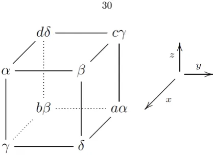
Figure 2.10: Stabilizer group generators forCSαβγδ andCAαβγδ.
Under the aforementioned constraints, one can see that the quantum code is described by 4 symplectic pairs α, β, γ, δ and the symmetric/antisymmetric nature of the code. We shall denote each of these codes as CA,Sαβγδ, where A stands for the antisymmetric code and S stands for the symmetric code. Without loss of generality, we shall assume that the system has a periodic boundary condition, with a fixed length in all three directions equal toL.
To compare our code to Haah’s code, Haah’s code has two local stabilizer generators per cube, which corresponds to the generators responsible for the protection against the bit flip and the phase flip error. Our code has one stabilizer generators for each cube. Some of Haah’s code is a CSS code, but all of our codes are non-CSS. Perhaps more importantly, the local particle dimension of Haah’s code is 22, while for our code it is a prime numberp. We shall in fact see that p= 2 inevitably leads to an existence of string logical operator, which confirms the numerical result by Haah.[48] As we shall see throughout the rest of this chapter, the main difference comes from the structure of the base field: the base field for our code is GF[p], while it is GF[22] for Haah’s code.
[image:39.595.221.425.247.421.2]of any string logical operator. Given a stabilizer code with cubic local generators, no string rule is implied by a simple algebraic constraint on the parameters of the code over a finite fieldFp. The
existence of the quantum code without string logical operator forp≥5 follows from this result. Another important point to discuss is that the codes described by a different set of symplectic pairs may give rise to the same code. Of course, the actual codeword of the quantum code will be not identical. However, they may be equivalent to each other under a local unitary transformation.1 If two quantum codesC1,C2can be mapped to each other via such local unitary transformation, we
shall denote their equivalence with the following notation:
C1∼=C2. (2.43)
Any two codes are equivalent to each other if they can be mapped by a lattice symmetry or a local unitary transformation. The lattice symmetry can be concisely represented as a permutation of the symplectic pairs α, β, γ, δ. The following lemma trivially follows from the definition of the code: the exchange of the symplectic pairs correspond to the rotation in the 3-space.
Lemma 8.
CA,Sαβγδ ∼=CA,Sσ(α)σ(β)σ(γ)σ(δ), (2.44)
whereσ∈S4 over a set{α, β, γ, δ}.
Any local Clifford transformation can be represented as an element ofSL(2, p).[115] One should also note that multiplying a nonzero element aof GF[p] does not change the code. It corresponds to merely changing the stabilizer elementsintosa.
Lemma 9. If∃a∈Fp, M ∈SL(2, p)such thataM{α, β, γ, δ}={α, β, γ, δ}
CA,Sαβγδ ∼=CA,Sα0β0γ0δ0, (2.45)
Finally, there is a subtle equivalence relation between the antisymmetric and the symmetric code. Instead of performing the same local unitary operation on all the qudits, one can imagine performing a unitary transformation on the even (or equivalently, odd) layer only, mappingA→ −A for A ∈ {α, β, γ, δ}. This maps the symmetric code to the antisymmetric code and vice versa in the bulk. However, if the length in the direction normal to these layers is odd, such an operation is ill-defined. In other words, there exists a unitary operation that relates the antisymmetric and symmetric code in the bulk ifLis an even number.
Combining these equivalence relations together, we can get the following result.
1Typically, local unitary transformation in this setting is used in a much stronger sense. More specifically, a local
Lemma 10. For d= 3 code satisfying the deformability condition, there are two symmetric code and two antisymmetric code up to lattice symmetry and local Clifford operation. The parameters of
the codes are{(1,0),(0,1),(1,1),(1,−1)} and{(1,0),(0,1),(1,1),(−1,1)}.
2.3.1
Sufficient condition for the no-string rule
Recall that the existence of a string logical operator is the bulk propertyof the code. That is, the formulation of the no-string rule does not involve anything about the boundary condition. Since there always exists an one-to-one correspondence between a symmetric code and an antisymmetric code that are described by the same symplectic pairs, it suffices to study only one of them for checking the absence of any string logical operator. If an antisymmetric code does not have any string logical operator, neither does the symmetric code with the same symplectic pairs. We shall obtain a sufficient condition for the code to not have any string logical operator for an antisymmetric code. The same statement for the symmetric code should follow trivially from this correspondence.
We first state our main result.
Theorem 3. ForCS,Aαβγδ, the maximum length of a nontrivial string logical operator with a widthw
is bounded by2w, if the following conditions are satisfied.
• Deformability condition : hA, Bi 6= 0∀A6=B,A, B∈ {α, β, γ, δ} • Absence of minima