Development of Interest in Science and Interest in Teaching Elementary Science: Influence of Informal, School, and Inquiry Methods Course Experiences

(1)

Physics and Astronomy Dissertations Department of Physics and Astronomy

8-7-2007

Hot Stars with Disks

Erika Dawn Grundstrom

Follow this and additional works at:https://scholarworks.gsu.edu/phy_astr_diss

Part of theAstrophysics and Astronomy Commons, and thePhysics Commons

This Dissertation is brought to you for free and open access by the Department of Physics and Astronomy at ScholarWorks @ Georgia State University. It has been accepted for inclusion in Physics and Astronomy Dissertations by an authorized administrator of ScholarWorks @ Georgia State University. For more information, please [email protected].

Recommended Citation

(2)

Abstract

The evolutionary paths of the massive O and B type stars are often defined by angular momentum transformations that involve circumstellar gas disks. This circumstellar gas is revealed in several kinds of observations, and here I describe a series of inves-tigations of the hydrogen line emission from such disk using detailed studies of five massive binaries and a survey of 128 Be stars. By examining three sets of spectra of the active mass-transfer binary system RY Scuti, I determined masses of 7.1_±1.2M

(3)

generation of a circumstellar disk. The disk of X Per appears to have grown to near record proportions and the X-ray flux has dramatically increased. Tidal interaction may generate a spiral density wave in the disk and cause an increase in Hα equiva-lent width and mass transfer to the compact companion. During the course of the analysis of the X-ray binaries, I developed numerical models for estimating the size of the Be star disks using just the Hα equivalent width. Finally, I present the results of a three year spectroscopic survey of both the Hαand Hγ regions of 128 Be stars. I find that the median fractional variation in the equivalent width of the disk emission lines is 15% over a two year period. I also find that two-thirds of the sample displays evidence of FeIIemission or absorption resulting from surrounding circumstellar ma-terial. Many candidates for non-radial pulsation and binary systems are also found. Spectra and notes for all of the sample stars are presented in an appendix.

(4)

Erika D. Grundstrom

A Dissertation

Presented in Partial Fulfillment of Requirements for the Degree of Doctor of Philosophy

in the College of Arts and Sciences Georgia State University

(5)

(6)

Erika D. Grundstrom

Major Professor: Committee:

Douglas R. Gies Gary Hastings Todd J. Henry Harold A. McAlister Geraldine J. Peters David W. Wingert

Electronic Version Approved:

(7)

Dedication

To my family:

my mother DorRayne, my father Don, and my siblings Tyan, Ian, and Svaya

You have always been there for me, supporting me and giving me that kick in the pants when I needed it!

(8)

shape me into who I am today, and people who have helped make this whole process of education a joy.

First and foremost, I’d like to thank my parents and my siblings. They have always been there for me and we always have such fun and interesting experiences. Throughout my life, they’ve always encouraged my schooling and my odd little inter-ests and all of the activities I do. Plus, they love to brag about me and that’s always nice! My extended family has always been supportive and curious about what I do and that’s the kind of encouragement a budding young scientist needs.

I’d also like to thank my advisor extraordinaire, Dr. Douglas R. Gies. He has always encouraged me to be a whole person and not chained to my desk (even if he may have wanted me to be ;) ) and has been extraordinarily supportive of my interest in education and education research.

A big thanks to my committee, Gary, Todd, Hal, Gerrie, Dave, and of course, Doug, for reading this! I hope you like it!

(9)

MissAngela has been my roommate, officemate, best friend, and belly dance part-ner for years now and that I’ll never forget and always cherish :)

The faculty and students at the University of Minnesota, especially my undergrad advisor, Dr. Larry Rudnick, prepared me so well for graduate school and I thank them. While at the U of M, I was an undergraduate mentee of graduate student Andrew Young and he’s been a friend and mentor throughout grad school, so I’d really like to thank him too.

Of course, a girl can’t be slaving away all the time so many thanks to all my swing dancing, belly dancing, booty-shakin’, and band-going friends in both Atlanta and Minnesota for helping keep me active and in the loop.

Many people at Georgia State have helped me along the way, teaching classes, making templates, going on observing trips, doing preliminary research... Many thanks to Alvin Das for the GSU dissertation template - it worked like a charm! Dr. David Wingert, Stephen Williams, and Tabby Boyajian have all gone on observ-ing runs with me and we’ve had a great time and learned a great deal in the process. Dr. Ginny McSwain, former roommate, now collaborator, has been a great friend and resource, plus she got me more telescope time! I’d also like to thank all of the graduate students in Doug’s Stellar Spectroscopy class for doing the preliminary work on the X-ray binaries, it was a great help. I’d especially like to thank the two un-dergraduates I have advised, John Helsel and Diana Gudkova - they have both done great work and it’s been so helpful!

(10)

(11)

Tables

2.1 RY Scuti Journal of Spectroscopy . . . 15

2.2 RY Scuti Supergiant Radial Velocity Line Sample . . . 34

2.3 RY Scuti Supergiant Radial Velocity Measurements . . . 36

2.4 RY Scuti Orbital Elements . . . 38

2.5 RY Scuti Hα Wing Velocities and Equivalent Widths . . . 42

2.6 RY Scuti Measurements of Massive Companion Features . . . 43

2.7 RY Scuti Summary of Radial Velocity Fits . . . 45

3.1 LS I +65 010 Observation Journal . . . 65

3.2 LS I +65 010 Radial Velocity and Equivalent Width Measurements . 67 3.3 LS I +65 010 Orbital Elements . . . 69

4.1 Be Stars with Interferometric Hα Measurements . . . 88

5.1 LS I +61 303 Radial Velocity and Hα Measurements . . . 95

5.2 LS I +61 303 Orbital Elements . . . 99

6.1 HDE 245770 and X Per Radial velocity and Hα measurements . . . . 123

6.2 HDE 245770 and X Per Adopted Stellar and Disk Parameters . . . . 128

(16)

7.5 Be Star Survey Fractional Variations in Equivalent Width . . . 195

7.6 Be Star Survey Statistics Regarding Fe II Features . . . 198

C.1 Be Star Survey - Red spectral line measurements . . . 235

C.2 Be Star Survey - Blue Spectral Line Measurements . . . 250

(17)

Figures

1.1 Diagram of a Roche surface in a binary . . . 3

1.2 Evolution of a close binary into a Be XRB . . . 4

1.3 Diagrams illustrating rotational broadening . . . 8

2.1 RY Scuti orbital phase variations in SiIV λ4088 . . . 18

2.2 RY Scuti orbital phase variations in HeI λ4387 . . . 20

2.4 RY Scuti orbital phase variations in HeI λλ4009,4026 . . . 22

2.8 RY Scuti orbital phase variations in SiIII λ4552 . . . 27

2.9 RY Scuti orbital phase variations in NII λ6610 . . . 28

2.10 RY Scuti nebular subtraction diagram . . . 30

2.11 RY Scuti orbital phase variations in Hα from the KPNO coud´e feed 31 2.12 RY Scuti orbital phase variations in Hα from FEROS . . . 32

2.13 RY Scuti orbital phase variations in HeII λ4686 . . . 33

2.14 RY Scuti radial velocity curve . . . 39

(18)

3.1 LS I +65 010 radial velocity curve . . . 70

3.2 LS I +65 010 temporal variations of Hα . . . 71

3.3 LS I +65 010 periodogram of the Hα equivalent width variations . . 73

3.4 LS I +65 010 long term variations in the X-ray flux and Hαequivalent width . . . 75

3.5 LS I +65 010 X-ray fluxes vs. orbital phase . . . 76

3.6 LS I +65 010 range of probable component masses . . . 78

4.1 Predicted Hα equivalent width vs. disk radius . . . 86

4.2 Comparison of interferometrically-determined disk sizes with the sim-ple model . . . 90

5.1 LS I +61 303 radial velocity curve . . . 99

5.2 LS I +61 303 average spectra showing normal and plummeted emission102 5.3 LS I +61 303 time variations in radio, X-ray and Hα strengths for three orbital periods . . . 103

5.4 LS I +61 303 orbital phase variations in Hα parameters . . . 105

5.5 LS I +61 303 orbital phase variations in radio, X-ray and Hα . . . . 106

5.6 LS I +61 303 time variations in radio, X-ray and Hα since 1988 . . 107

5.7 LS I +61 303 predicted disk radius vs. Hα equivalent width . . . . 109

6.1 HDE 245770 spectra during disk near-disappearance . . . 120

6.2 HDE 245770 average spectra from each run . . . 121

6.3 X Per average spectra from each run . . . 122

6.4 Relation between Hα equivalent width and disk radius . . . 128

(19)

6.6 HDE 245770 orbital phase variations of the X-ray light curves . . . 136

6.7 X Per time evolution of the X-ray flux, photometric magnitude, and disk radius . . . 138

6.8 X Per orbital phase variations of the X-ray light curves . . . 140

6.9 X Per radial velocity curve from IUE data . . . 145

6.10 X Per mass plane diagram . . . 146

7.1 Diagram of double-peaked emission . . . 149

7.2 Be Star Survey “normal” stars . . . 161

7.3 Be Star Survey “squarish” stars . . . 162

7.4 Be Star Survey “emission shell” stars . . . 163

7.5 Be Star Survey “shell” stars . . . 164

7.6 Be Star Survey quadruple plot example . . . 166

7.7 Be Star Survey comparison with Deneb . . . 178

7.8 Be Star Survey cross-correlation functions compared to Deneb . . . 179

7.9 Be Star Survey correction inWλ of the hydrogen lines vs. Teff . . . 181

7.10 Be Star Survey ratio of Wλ(HeI)/Wλ(MgII) vs. Teff . . . 182

7.11 Be Star Survey Wλ(Hγ) vs. Wλ(Hα) . . . 185

7.12 Be Star Survey Wλ(FeII CCF) vs. Wλ(Hα) . . . 186

7.13 Be Star Survey V sinivs. FWSM(HeI) . . . 191

7.14 Be Star Survey V sinivs. FWSM(MgII) . . . 192

7.15 Be Star Survey FWSM(HeI)/FWSM(MgII) vs. V sini . . . 194

7.16 Be Star Survey cumulative distributions of the fractional variations in equivalent width . . . 196

7.17 Example of an extremely variable star - Pleione . . . 197

7.18 Be Star Survey π Aqr HeI λ6678 plots . . . 200

7.19 Be Star Survey π Aqr plot of SiIII . . . 201

A.1 Wing velocity measurement diagram . . . 224

(20)

C.5 Plot of all blue spectra of HD005394 . . . 282

C.6 Quadruple plot of HD006811 . . . 284

C.23 Plot of the averages of blue runs of HD021362 . . . 313

(21)

C.38 Plot of the averages of blue runs of HD023862 . . . 342

(22)

(23)

(24)

(25)

(26)

ASM All-Sky Monitor on the Rossi X-ray Timing Explorer

BeXRB Be X-ray Binary

CCD Charged Coupled Device

CCF cross-correlation function

FWHM full-width at half-maximum

FWSM full-width of the second moment at half-maximum

HJD Heliocentric Julian Date

HWHM half-width at half-maximum

IDL Interactive Data Language

IR infrared

IRAF Image Reduction and Analysis Facility

IUE International Ultraviolet Explorer

JD Julian Date

KPNO Kitt Peak National Observatory

keV kiloelectron-volts

(27)

LTE local thermodynamic equilibrium

MAST Multimission Archive at Space Telescope

NASA National Aeronautic and Space Administration

NOAO National Optical Astronomy Observatory

NRP non-radial pulsation

pc parsec

RXTE Rossi X-ray Timing Explorer

RV radial velocity

S/N signal-to-noise ratio

(28)

1.1 Massive Stars

The stars with O and B-type spectral classifications are much hotter, brighter, and more massive than our Sun. They evolve very quickly compared to cooler, less massive stars. Because they have short lifetimes, O and B stars are usually found in groups in star-forming regions and at a variety of stages in the evolutionary track of a star. Due to their intrinsic brightness, their groupings, and their short lifetimes, these massive stars provide excellent laboratories for studying stellar evolution.

Throughout this dissertation, I will be focusing on B type stars, and therefore I will first describe the properties of the B stars. They have masses between 3 and 20 M, temperatures of 10000 to 30000 K, radii between 2.5 and 6 R (for the

unevolved, “main sequence” stars), and lifetimes of 6 million to 600 million years (the more massive, the shorter the lifetime). For comparison, our Sun’s lifetime is 10 billion years. The hottest B stars are B0 and are often called “early”-type in the literature while the coolest B stars, B9, are called “late”-type. Another part of a star’s classification is its luminosity class. From brightest to dimmest, the classes are

(29)

I, II, III, IV, and V. The class V (dwarf) stars are the unevolved main sequence stars and are the most plentiful. Class I stars are supergiants, II are bright giants, III are giants, and IV are subgiants.

The lifetime quoted above is the main sequence lifetime. A star on the main sequence is fusing hydrogen into helium in its core. Once the star has exhausted its fuel supply and can no longer fuse hydrogen, the radiation and gas pressure that kept the star from collapsing due to gravity is gone and the stellar core begins to collapse. This heats the core and makes it denser, which provides an environment for fusion of helium. Helium starts fusing and the star expands. This cycle of fusion, exhaustion, collapse, and fusion of a new element continues until either the collapse of the core cannot restart fusion or until the core has fused to iron. Iron is the “magic” element, as fusion of iron does not release energy, it requires energy. For stars with masses of about 3 to about 9 M, fusion stops at carbon, oxygen, and nitrogen and the remnant of this star is a white dwarf (supported by electron degeneracy pressure). Above 9 M, the core can fuse until iron forms, then fusion stops and there is no

more pressure to keep the star from collapsing completely, and the star experiences a core-collapse supernova event. For stars with masses of about 9 to 30-40 M, the remnant is a neutron star (supported by neutron degeneracy pressure). For stars with masses greater than 30-40 M (i.e., O stars), the remnant is a black hole.

(30)

[image:30.612.227.415.112.245.2]

Figure 1.1: Diagram illustrating gravitational equipotential contours around two stars with

massesM1 andM2 that are a distanceaapart. They are rotating around the center of mass

(theplus sign) with an angular velocityΩ. The two parts of thelopsided figure-eightare the

respective Roche lobes and where they join is the inner Lagrangian point (L1). Image from

Bowers & Deeming (1984).

(31)

[image:31.612.207.452.104.400.2]

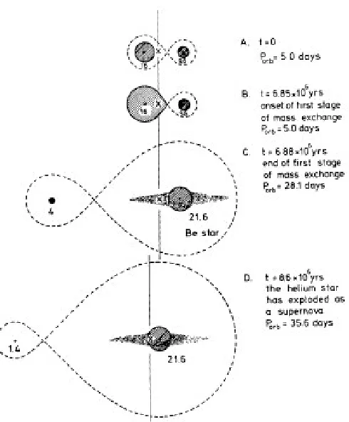
Figure 1.2: The evolution of a close binary system into a Be X-ray binary system. Image from Rappaport & van den Heuvel (1982).

in later chapters. Material from the outflowing disk may transfer back onto the now remnant companion and an accretion disk will form. This accretion disk can get hot enough to produce X-rays.

1.2 Observational Techniques in Spectroscopy

(32)

absorption spectrum. Should the light source be a hot (i.e., energized), thin gas, it will emit photons at the wavelengths corresponding to the energy released when electrons move to a lower energy level, creating an emission spectrum. As no two elements have the same energy levels for their electrons, no two elements have the same spectral signature.

The spectrum of a star is an absorption spectrum as the source of light (produced by fusion at the core) is surrounded by a cooler gas (the stellar atmosphere). There are many different gas species in the atmosphere of a star andtherefore many spectral signatures are superposed on one another. The most important spectral lines in my study of hot stars are produced by hydrogen, helium, carbon, oxygen, nitrogen, silicon, and iron.

The spectral lines of hydrogen that are at optical wavelengths are called the Balmer lines. These lines are produced by electrons going into and out of energy level 2 from and to higher energy levels. Hα (a red line) is produced by the electron transition between levels 2 and 3 (absorption is from 2 to 3, emission from 3 to 2). Hβ (a blue-green line) is the transition between 2 and 4, and Hγ (a violet line) is between levels 2 and 5. Throughout this dissertation, I rely heavily on the Hα and Hγ lines.

1.2.1 Absorption Line Studies

(33)

tempera-ture of a star. For instance, in B stars, the depths of the hydrogen absorption lines change a great deal with temperature – the hotter the star, the smaller (i.e., narrower and shallower) the lines (so B9 stars have very deep and broad hydrogen lines while B0 stars have relatively small hydrogen lines). Other lines also display temperature sensitivity – Mg II gets stronger the cooler the star is, Si III and He II start ap-pearing at hotter temperatures, and HeI gets stronger, peaks, and gets weaker with increasing temperature. Therefore, if one knows the patterns, one may estimate the temperature, which is considered a fundamental parameter of a star.

The gravitational force at the photospheric surface of the star is measured as logg (g expressed in cgs units ofcm s−2_{). The bigger the number, the more surface}

gravity there is. More gravitational pressure will cause atoms to collide more, which will broaden the spectral line. For supergiant stars, logg is small, about 3.0 (as the surface of the star is far from the gravitational center of the star) and the spectral lines are not broad. For main sequence stars, logg is relatively high (about 4.0 or 5.0) so the lines will look broader. The value of logg is also considered a fundamental parameter of a star because it is linked to mass, the most fundamental of all stellar characteristics.

If one examines the spectrum of superposed spectral lines of different elements, one may determine the chemical composition of the star. The chemical composition of a star is measured relative to the solar abundance (as the Sun is the best studied star). Should the relative size of the absorption line of, say, helium be stronger than hydrogen for the temperature of the star, then we would say the star is helium enriched (or perhaps hydrogen deficient, depending on the abundances derived from other lines).

(34)

The non-relativistic version of the Doppler formula is

v = λ−λ0

λ0

c (1.1)

wherev is the velocity of the light source, λis the observed wavelength,λ0 is the rest

wavelength, and cis the speed of light. As a star rotates, part of it is moving toward the observer and part is moving away, so some of the light is shifted blueward and some is shifted redward. This shifting due to rotation will broaden any stellar spectral feature. The left side of Figure 1.3 illustrates how Doppler-shifted light from segments of a stellar surface can combine to make a broadened composite. The portions of the star in regions I and V are moving the fastest so they provide the most shifted light. On the right side of Figure 1.3, the effects of rotational broadening are shown for a computed profile on the top and then in the lower two panels, two stars of the same type but different rotation speeds (the slower one is on the bottom). The projected rotational velocity V sini is another fundamental parameter of a star.

(35)

[image:35.612.118.525.109.406.2]

Figure 1.3: Left: Illustration showing how the addition of all areas of a rotating star contribute to the broadening of a spectral line (from http://www.konkoly.hu/staff/kovari/research.html). Right: Diagram from Gray (1992). The top panel shows computed profiles to illustrate

broad-ening by rotation and the labels denote the rotation speed in km s−1_{. The bottom two panels}

show two stars of the same spectral type but HR 9024 rotates faster.

when the two stars are closest in their orbits. This value can be different depending on when the star was observed, as it is used as a starting point to determine where a star is in the binary orbit at the actual time of observation. Orbital phase is defined as the fractional part ofφ = (t₋T)/P for any given timet. The fourth element is the eccentricity e. Eccentricity is a measure of how non-circular (or “elliptical”) an orbit is, where e= 0 is a perfect circle and e= 1 is a straight line (the circle is completely “squished”). Denoting the semi-major axis of the orbit, the fifth element a is often given in astronomical units and is measured in the plane of the orbit. The quantity

(36)

crosses the plane of the sky (thus there are two). This angle is measured in the plane of the sky from north to a node (should be less than 180◦ _{unless one can determine}

which one corresponds to the star moving away from the observer).

Should the binary system have enough spectroscopic information regarding shifts in spectral features from a “rest” wavelength (radial velocities), one may make a radial velocity curve. If a star is moving quickly around it’s companion, spectral features will be shifted according to the Doppler formula above. There are two parameters that characterize the radial velocity curve, K and γ. K is the semi-amplitude of the curve in km s−1_{. The faster a star orbits, the larger} _K _{is. The center-of-mass (or}

systemic) velocity is denoted by γ. If this number is positive, the binary system is moving away from the observer, if negative, toward. If one has radial velocity curves for both components of the binary, one may also determine the mass ratioqby taking the inverse ratio of theK measurements (as the more massive one will have a smaller semi-amplitude and vice versa).

1.2.2 Emission Line Studies

(37)

(together with absorption lines) to study the radial velocity shifts of the star or of the circumstellar gas itself.

1.3 Studies Presented Here

(38)

Abstract

The massive interacting binary RY Scuti is an important representative of an active mass-transferring system that is changing before our eyes and which may be an example of the formation of a Wolf-Rayet star through tidal stripping. Utilizing new and previously published spectra, we1_{present examples of how a number of illustrative}

absorption and emission features vary during the binary orbit. We identify spectral features associated with each component, calculate a new, double-lined spectroscopic binary orbit, and find masses of 7.1_±1.2 M for the bright supergiant and 30.0_± 2.1 M for the hidden massive companion. Through tomographic reconstruction of the component spectra from the composite spectra, we confirm the O9.7 Ibpe spectral class of the bright supergiant and discover a B0.5 I spectrum associated with the hidden massive companion; however, we suggest that the latter is actually the spectrum of the photosphere of the accretion torus immediately surrounding the 1_{Grundstrom, E. D.; Gies, D. R.; Hillwig, T. C.; McSwain, M. V.; Smith, N.; Gehrz, R. D.; Stahl,} O.; Kaufer, A. - published as Grundstrom et al. (2007d)

(39)

massive companion. We describe the complex nature of the mass loss flows from the system based upon recent hydrodynamical models and find RY Scuti has matter leaving the system in two ways: 1) a bipolar outflow from winds generated by the hidden massive companion, and 2) an outflow from the bright O9.7 Ibpe supergiant in the region near the L2 point to fill out a large, dense circumbinary disk. This circumbinary disk (radius ≈1 AU) may feed the surrounding double-toroidal nebula (radius ≈2000 AU).

2.1 Introduction

RY Scuti (HD 169515) is a distant (1.8 ± 0.1 kpc; Smith et al. 2002) and massive eclipsing binary system with an orbital period of 11.12445 days (Kreiner 2004). Anal-ysis of the light curve indicates that at least one of the components fills its Roche lobe. The present configuration may be semi-detached (Cowley & Hutchings 1976), overcontact (Milano et al. 1981; Djuraˇsevi´c et al. 2001), or one with the more mas-sive component embedded in an opaque, optically thick disk (King & Jameson 1979; Antokhina & Kumsiashvili 1999). The binary appears to be in an advanced stage of evolution, and it has ejected gas into a young (∼130 year old; Smith, Gehrz, & Goss 2001), double-toroidal emission nebula. The≈ 2000 AU nebula is angularly resolved in radio images (Gehrz et al. 1995), infrared images (Gehrz et al. 2001), and inHubble

Space Telescope Hα images (Smith et al. 1999, 2001, 2002). Because the nebula is so

young and the star system is still in an active Roche-lobe overflow phase, RY Scuti is a powerful laboratory for studying non-spherical mass and angular momentum loss in interacting binaries.

(40)

com-“massive companion.” However, the actual masses of the stars in this system are debatable. The radial velocity curve of the supergiant is reasonably well established, but the results for the massive companion depend critically on what spectral fea-tures one assumes are associated with that star. As these feafea-tures are difficult to observe and interpret, the estimated mass range has been huge. For example, Pop-per (1943) arrived at a total system mass in excess of 100 M. Later investigators found lower values: Cowley & Hutchings (1976) estimated masses of 36 and 46 M, Skul’Skii (1992) found 8 and 26M, and Sahade, West, & Skul’Skii (2002) estimated 9 and 36 M (for the supergiant and massive companion, respectively, in each case). There are a number of important photometric studies (e.g., ranging from the discov-ery by Gaposchkin & Shapley 1937 through photoelectric investigations by Giuricin & Mardirossian 1981 and Milano et al. 1981, and up to the most recent multi-color work by Djuraˇsevi´c et al. 2001); however the results differ with regard to the as-sumed binary configuration and depend sensitively on the mass ratio adopted from spectroscopy.

This unique system is representative of the short-lived, active mass transfer stage in the evolution of massive binaries. Theoretical models (Petrovic, Langer, & van der Hucht 2005) indicate most of the mass transfer occurs during a brief (≈104 _yr),

(41)

belong to the observed class of W Serpentis binaries (Tarasov 2000). Only the mass donor star is visible in the spectra of these binaries, and the more massive gainer star is hidden in a thick accretion disk (one source of emission lines in the spectra). The mass transfer process is complex and leaky, and a significant fraction of the mass loss leaves the system completely (as described by Harmanec 2002 for the best known object of the class, β Lyr). The mass donor may eventually lose its entire hydrogen envelope and emerge as a Wolf-Rayet star. Therefore, a system like RY Scuti may be the progenitor of a WR+O binary system (Giuricin & Mardirossian 1981; Antokhina & Cherepashchuk 1988; Smith et al. 2002).

(42)

Range Optical Spectrograph (FEROS) mounted on the 1.52 m telescope of the Euro-pean Southern Observatory (ESO) at La Silla, Chile (see Smith et al. 2002). Also in 1999, we obtained 40 moderate dispersion spectra (in the red region surrounding Hα) using the Kitt Peak National Observatory coud´e feed 0.9 m telescope. Finally, in 2004 we used the CTIO 1.5 m telescope2 _{and Cassegrain spectrograph to obtain ten blue}

spectra of moderate resolution covering one orbital period. Table 2.1 contains run number, dates, spectral coverage, spectral resolving power, number of spectra, tele-scope, spectrograph grating, and CCD detector used in each case. Exposure times were generally limited to 30 minutes or less. Each set of observations was accom-panied by numerous bias, flat-field, and ThAr comparison lamp calibration frames. Furthermore, we obtained multiple spectra each night of the rapidly rotating A-type star ζ Aql for removal of atmospheric water vapor and O2 bands in the red spectra

made with the KPNO coud´e feed.

Table 2.1: Journal of Spectroscopy

Run Dates Range Resolving Power Number of Observatory/Telescope/ Number (HJD-2,450,000) (˚A) (λ/4λ) Spectra Spectral Grating/CCD 1 . . . 1354.7 – 1354.8 6431 – 6785 5440 2 KPNO/0.9m/RC181/TI5 2 . . . 1355.7 – 1364.9 5405 – 6743 3950 32 KPNO/0.9m/RC181/F3KB 3 . . . 1373.7 – 1394.6 3600 – 9200 48000 17 ESO /1.5m/FEROS/EEV 2×4K 4 . . . 1421.8 – 1429.7 5397 – 6735 4050 6 KPNO/0.9m/RC181/F3KB 5 . . . 3152.9 – 3164.9 4068 – 4738 2430 10 CTIO/1.5m/#47II/Loral 1K

The spectra from all the telescopes were extracted and calibrated using standard routines in IRAF3_{. All the spectra were rectified to a unit continuum by fitting}

line-2_{operated by the SMARTS consortium}

(43)

free regions. We removed the atmospheric lines from the red coud´e feed spectra by creating a library of ζ Aql spectra from each run, removing the broad stellar features from these, and then dividing each target spectrum by the modified atmospheric spectrum that most closely matched the target spectrum in a selected region dom-inated by atmospheric absorptions. In a few cases this resulted in the introduction of spectral discontinuities near the atmospheric telluric lines, and these were excised by linear interpolation. We did not attempt any removal of atmospheric lines for the FEROS spectra, but some problem sections in the echelle-overlap regions were excised via linear interpolation. The spectra were then transformed to a common heliocentric wavelength grid for each of the FEROS, KPNO coud´e feed, and CTIO 1.5 m runs. We show several examples of the final spectra in the next section.

2.3 Spectral Variations with Orbital Phase

(44)

variability observed, and in the following sections we analyze in detail the Doppler velocity shifts related to features associated with the supergiant (§2.4) and its massive companion (§2.5).

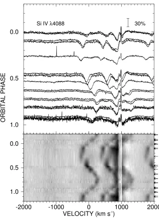
We begin with some examples from the high resolution FEROS spectra. The SiIV

λ4088 absorption feature is one of only a small number of spectral lines formed in the photosphere of the supergiant that is not filled in or affected by nebular emis-sion. We show the orbital phase variations of this line (and the nearby N III λ4097 and Hδ lines) in Figure 2.1 as a function of heliocentric radial velocity for Si IV

λ4088. In this and the next figures we adopt the orbital period from Kreiner (2004) ofP = 11.12445 d and the epoch of phase zero as the supergiant superior conjunction at TSC = HJD 2,451,396.71 (derived in §2.4). The upper portion of Figure 2.1

shows the SiIVprofiles with their continua aligned with the phase of observation (in-creasing downwards) while the lower portion shows the spectra as a gray-scale image interpolated in phase and velocity. Features moving with the radial velocity curve of the supergiant will have a characteristic “S” shape in this image. The break in the continuity of the “S” curve near phaseφ = 0.35 is due to the unfortunate gap in our phase coverage near there and to the simplicity of the interpolation scheme. The Si IV λ4088 feature appears to be useful for the radial velocity measurement of the supergiant, although we find that the depth of the line varies with phase, weakening at φ = 0.0 and strengthening at φ = 0.5. There is no obvious evidence of a reverse “S” feature that would correspond to the motion of the massive companion (although a weak feature is present; _§2.6).

(45)

0.0

0.5

1.0

ORBITAL PHASE

30% Si IV λ4088

-2000 -1000 0 1000 2000

VELOCITY (km s-1₎

0.0

0.5

[image:45.612.163.479.109.541.2]

1.0

Figure 2.1: The orbital phase variations in the Si IV λ4088 absorption line in the FEROS

spectra of RY Scuti are shown in linear plots (top panel) and as a gray-scale image (lower panel).

The intensity in the gray-scale image is assigned one of 16 gray levels based on its value between the minimum (dark) and maximum (bright) observed values. The intensity between observed spectra is calculated by a linear interpolation between the closest observed phases

(shown by arrows along the right axis). The feature centered at 0 km s−1 _{is Si} _IV _λ₄₀₈₈_,

and to the right is NIIλ4097, Hδ λ4101(exhibiting both photospheric absorption and nebular

emission features), and SiIVλ4116(far right edge).

(46)

(47)

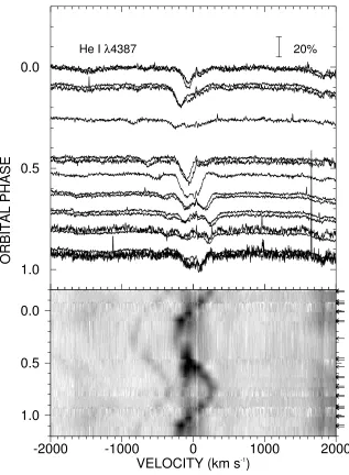
0.0

0.5

1.0

ORBITAL PHASE

20% He I λ4387

-2000 -1000 0 1000 2000

VELOCITY (km s-1₎

0.0

0.5

[image:47.612.164.481.154.586.2]

1.0

Figure 2.2: The orbital phase variations in the He Iλ4387singlet shown in the same format

as Fig. 2.1. This feature strengthens at conjunctions and develops a blueshifted absorption

feature afterφ= 0.5. Traces of the radial velocity curve of the fainter massive companion are

seen especially afterφ= 0.5, however, this feature is not used in the radial velocity analysis

due to the aforementioned blueshifted absorption feature. The fainter absorption feature just

(48)

0.0

0.5

1.0

ORBITAL PHASE

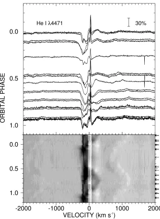
30% He I λ4471

-2000 -1000 0 1000 2000

VELOCITY (km s-1)

0.0

0.5

[image:48.612.164.479.164.594.2]

1.0

Figure 2.3: The orbital phase variations in the HeIλ4471triplet shown in the same format as

Fig. 2.1. This line has a stronger blueshifted absorption feature afterφ= 0.5that transforms

(49)

0.0

0.5

1.0

ORBITAL PHASE

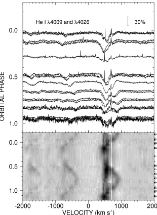
30% He I λ4009 and λ4026

-2000 -1000 0 1000 2000

VELOCITY (km s-1)

0.0

0.5

[image:49.612.165.475.166.591.2]

1.0

Figure 2.4: The orbital phase variations in the He Iλ4009singlet (at ₋634 km s−1_{) and the}

HeIλ4026triplet (at+634 km s−1_{) shown in the same format as Fig. 2.1. He}_I_λ₄₀₀₉_exhibits

the same behavior as He Iλ4387(also a singlet). He Iλ4026behaves like He Iλ4471(also a

(50)

0.0

0.5

1.0

ORBITAL PHASE

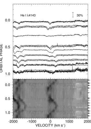
30% He I λ4143

-2000 -1000 0 1000 2000

VELOCITY (km s-1)

0.0

0.5

[image:50.612.165.480.157.599.2]

1.0

Figure 2.5: The orbital phase variations in the He Iλ4143singlet shown in the same format

as Fig. 2.1. It behaves as the HeIλ4387singlet does. The two absorption features at₋1953

and₋1591 km s−1_{are Si} _IV_λ₄₁₁₆_{and He}_I_λ₄₁₂₁_{(this helium feature is also a singlet). The}

(51)

0.0

0.5

1.0

ORBITAL PHASE

30% He I λ4921

-2000 -1000 0 1000 2000

VELOCITY (km s-1)

0.0

0.5

1.0

Fig. 2.1. This line behaves in the same manner as the HeIλ4471triplet. The feature at+600

(52)

0.0

0.5

1.0

ORBITAL PHASE

30% He I λ4713

-2000 -1000 0 1000 2000

VELOCITY (km s-1₎

0.0

0.5

1.0

Fig. 2.1. This line behaves in the same manner as the HeIλ4471triplet. The broad emission

feature on the left is HeIIλ4686which is discussed further in Fig. 2.13. Strong [FeII] nebular

emission features are present at−810 and+1450 km s−1_{. The faint absorption at}₊_{840 km s}−1

(53)

Figure 2.8 shows the orbital variations in the triplet Si III λλ4552,4567,4574 in the velocity frame of SiIII λ4552. The supergiant component appears to be present and undergoes the same kind of strengthening at conjunctions seen in the HeIlines. However, each of the triplet members also shows a broad shallow feature that moves in the manner expected for the massive companion. Thus, our observations confirm the detection of this second component that was discovered by Skul’Skii (1992).

(54)

0.0

0.5

1.0

ORBITAL PHASE

20% Si III λ4552

-2000 -1000 0 1000 2000

VELOCITY (km s-1₎

0.0

0.5

1.0

Figure 2.8: The orbital phase variations in the SiIIIλ4552line in the same format as Fig. 2.1.

All of the triplet SiIIIλ4552,4567,4574(at 0, 1004, and 1459 km s−1_{, respectively) components}

show dramatic strengthening at the conjunctions and display a broad, shallow feature moving

in anti-phase as expected for the massive companion. The absorption feature at−726km s−1

(55)

0.0

0.5

1.0

ORBITAL PHASE

30% N II λ6610

-2000 -1000 0 1000 2000

VELOCITY (km s-1)

0.0

0.5

1.0

Figure 2.9: The orbital phase variations in the emission feature of N II λ6610shown in the

same format as Fig. 2.1 although the plot is not centered on the feature as the very strong

Hα and [N II] features are nearby. The dark absorption line at ₋725 km s−1 _{is the diffuse}

(56)

plus a strong but narrow component formed in the double-toroidal nebula (Smith et al. 2002). Therefore, in order to isolate the emission component near the binary, we had to remove the nebular components of Hα and the nearby [N II] λλ6548,6583 lines. This removal process was done by scaling the [N II] λ6583 line in each spectrum to the appropriate size (of either Hα or [N II] λ6548) using the equivalent widths of these lines from Smith et al. (2002), shifting the rescaled line to the location of the line to be removed, and then subtracting it from the spectrum. This process was done interactively and included small adjustments in the scaling and shifting parameters to optimize the subtraction. This procedure was carried out using the IDL program subcs-v3.pro given in Appendix B. An example of the spectrum before and after subtraction is given in Figure 2.10. The resulting subtracted Hα profiles, based upon the large set of KPNO coud´e feed spectra, are illustrated as a function of orbital phase in the left panel of Figure 2.11. We also show the one spatially resolved HST spectrum of the central binary from the work of Smith et al. (2002) (which has no nebular emission present) that verifies that our line subtraction technique creates difference profiles with the appropriate shape. The emission strength appears to be much stronger at the conjunction phases, but this is due mainly to the drop in the continuum flux at those eclipse phases and our normalization of the emission strength to this varying continuum level. The right panel in Figure 2.11 shows a representation of the Hα profiles relative to a constant flux continuum we made by rescaling the emission flux by a factor

(57)

6550 6600 6650 6700 Wavelength (Angstroms)

0 2 4 6 8

[image:57.612.176.491.113.358.2]

Relative Flux

Figure 2.10: Diagram showing the remainder from the subtraction of the nebular lines in Hα

and HeIλ6678and of the [NII]λλ6548,6583lines for the data set from the KPNO coud`e feed.

Thesolid lineis the original, unaltered spectrum, and thedotted lineis the spectrum with the nebular features removed.

where V is the V-band magnitude at the orbital phase of observation (found by interpolation in the light curve data from Djuraˇsevi´c et al. 2001) and V = 9.03 corresponds to the maximum brightness of the system at quadrature phases. The Hα emission feature appears broad (spanning over 1000 km s−1_{) and approximately}

constant in strength and position in this version. There is often a weak, blueshifted absorption component present (with a radial velocity of ≈ −150 km s−1_{) that gives}

the profile a P Cygni appearance. Similar results were seen in the Hα difference profiles formed from the smaller set of FEROS spectra using using the IDL program

subcsFEint.pro given in Appendix B. The orbital phase variations are shown in

Figure 2.12.

(58)

0.5

1.0

ORBITAL PHASE

-1000 -500 0 500 1000

VELOCITY (km s-1₎

0.0

0.5

1.0

0.5

1.0

ORBITAL PHASE

-1000 -500 0 500 1000

VELOCITY (km s-1₎

0.0

0.5

1.0

Figure 2.11: The orbital variations in the Hαprofiles after subtraction of the nebular

compo-nent (based upon the KPNO coud´e feed set of spectra). The dashed line atφ= 0.15is a single

HSTspectrum of the central binary exclusive of the surrounding nebula, and the good match

to our spectra at that phase indicates that the nebular subtraction method is reliable. The

left hand panel shows the profiles normalized to the observed continuum (lower nearφ= 0.0

andφ = 0.5) while the right hand panel shows the emission rescaled to a constant reference

continuum. The net Hαprofile is approximately stationary and has high velocity wings that

move in anti-phase to the supergiant’s radial velocity curve.

FWHM = 45 km s−1 _{to improve the otherwise noisy appearance. This feature is}

(59)

0.0

0.5

1.0

ORBITAL PHASE

70% Hα

-1000 -500 0 500 1000

VELOCITY (km s-1)

0.0

0.5

1.0

Figure 2.12: The orbital variations in the Hαprofiles after excising the nebular component

(60)

0.0

0.5

1.0

ORBITAL PHASE

10% He II λ4686

-1000 -500 0 500 1000

VELOCITY (km s-1)

0.0

0.5

1.0

Figure 2.13: The orbital phase variations of the broad and weak He II λ4686emission line.

It appears brighter atφ= 0.0and shows a hint of the anti-phase motion associated with the

(61)

2.4 Radial Velocity Curve of the Supergiant

The radial velocity shifts of the supergiant are readily apparent in many lines, and given the quality and number of the new spectra we decided to measure the radial velocities and reassess the orbital elements. We measured relative radial velocities by cross-correlating each spectrum with a template spectrum. For the FEROS and CTIO spectra, this template spectrum was generated from the non-LTE, line-blanketed model atmosphere and synthetic spectra grid from Lanz & Hubeny (2003) using

Teff = 30000 K and logg = 3.0, which are appropriate values for an O9.7 Ib star

(Herrero et al. 1995). This template was rotationally broadened (§2.5) and also smoothed to the instrumental resolution of the FEROS or CTIO spectra. First, we removed certain interstellar features by forming an average interstellar spectrum from the mean of the entire set and then dividing each spectrum by the average interstellar spectrum. Because the spectrum of RY Scuti contains so many stationary nebular lines and possible features from the massive companion, we restricted the wavelength range for the cross-correlation to regions surrounding a set of absorption lines that appeared to be free of line blending and that were clearly visible throughout the orbit. The main features in the selected regions are summarized in Table 2.2.

Table 2.2: Supergiant Radial Velocity Line Sample

Telescope Run Line Regions

ESO 1.5 m Si IVλ4088; Si IVλ4116, He Iλ4121; N III λλ4510,4514,4518;

CTIO 1.5 m Si IVλ4088; Si IVλ4116, He Iλ4121; N III λλ4510,4514,4518;

KPNO CF N IIλ6610 (em.); Si IVλ6701 (em.)

(62)

well separated from any component from the massive companion. Once again, we first removed interstellar features, then selected regions free from nebular lines for the cross-correlation. Once we performed the cross-correlation, we determined the absolute radial velocity of the template spectrum by fitting the core of the emission lines (N II λ6610 and Si IV λ6701) with a parabola and determined the shift from the rest wavelengths. We added the radial velocity of the template to all the relative velocities to place them on an absolute scale.

Because the velocities from the different runs are based upon measurements of dif-ferent lines in the template and individual spectra, we anticipated that there might be systematic differences in the zero-points of each set. We began by making inde-pendent circular orbital fits for each set, and indeed we found the systemic velocityγ

for the FEROS set was offset by −20.6 km s−1 _{from the resulting systemic velocities}

for the KPNO and CTIO sets. As the latter were closer to the nebular systemic velocity (20_±3 km s−1_{; Smith et al. 2002) and based upon more observations, we}

arbitrarily adjusted the FEROS measurements by adding 20.6 km s−1 _{to bring them}

(63)

red spectra, so the velocity error is estimated as the larger of the difference between the two measurements or the mean value of _|Vi−Vi+1|/

√

2 from closely spaced pairs of observations.

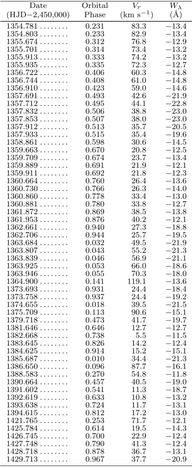
Table 2.3: Supergiant Radial Velocity Measurements

HJD Orbital Vr σ O−C

(−2,450,000) Phase (km s−1₎ _{(km s}−1₎ _{(km s}−1₎ _Telescope

(64)

We determined revised orbital elements using the the nonlinear, least-squares, fit-ting code of Morbey & Brosterhus (1974). Because the errors associated with each run are different, we assigned each measurement a weight proportional to the inverse square of the measurement error. The orbital period was fixed at P = 11.12445 days as found by Kreiner (2004) from contemporary eclipse timing observations over a long time base. We made both eccentric and circular orbital solutions, but we think the eccentric solution, while formally statistically significant according to the test of Lucy & Sweeney (1971), is probably spurious. Harmanec (1987) found that gas streams and circumstellar matter (both present in RY Scuti) can distort spec-troscopic features in mass-transferring binaries because they add emission to said features in non-symmetric ways. Such distortions can lead to skewed radial velocity results and thus artificial eccentricities (Lucy 2005). A zero eccentricity is consistent with predictions for Roche lobe overflow systems where the tidal effects are expected to circularize the orbit and synchronize the rotational and orbital periods. The final orbital elements from both the circular and eccentric solutions are presented in Ta-ble 2.4 together with solutions from Sahade et al. (2002) and Skul’Skii (1992). The epoch TSC refers to the time of supergiant superior conjunction (close to the time

(65)

(2002). We suspect the difference is due to the lack of orbital phase coverage in the observations of Sahade et al. (2002) in the ascending portion of the velocity curve.

Table 2.4: Orbital Elements for RY Scuti

Element Circular Elliptical Sahade et al. (2002) Skul’skii (1992)

P (days) . . . 11.12445a _11.12445a _11.124646a _11.1250a

TSC(HJD–2,400,000) 51396.71±0.02 · · · 44777.9±1.0

T (HJD–2,400,000) . . · · · 51395.68±0.40 45107.74 · · ·

e . . . 0 0.05±0.01 0.16±0.04 0

ω(deg) . . . · · · 57±13 345±15 · · ·

KSG(km s−1) . . . 249±3 247±3 273±14 235±3

KM C (km s−1) . . . 59±9 · · · 71±9 71±2

γSG(km s−1) . . . 11±2 12±2 17±5 9±2

γM C (km s−1) . . . −20±9 · · · 11±2

r.m.s.SG(km s−1) . . . 19 17 · · · ·

r.m.s.M C (km s−1) . . 25 · · · ·

a(R) . . . 69.9±2.3 · · · 77±4 68

q=MM C/MSG . . . 4.2±0.7 · · · 3.9±0.5 3.3±0.1

MSG(M) . . . 7.1±1.2 · · · 10.2±1.7 8

MM C (M) . . . 30.0±2.1 · · · 39±4 26 a _Fixed

2.5 Nature of the Massive Companion

Very little is known about the massive companion because it is difficult to find its associated features in the spectrum (probably because the massive companion is en-shrouded in a thick accretion disk; _§2.7). We can make an approximate estimate for the expected semiamplitude of motion for the massive companion using a geomet-rical argument to find the mass ratio, q = MM C/MSG. Let us assume the

(66)

0.0 0.5 1.0 ORBITAL PHASE

-200 -100 0 100

RADIAL VELOCITY (km s

Figure 2.14: The radial velocity curve and measurements for several spectral components

(where φ = 0.0 corresponds to supergiant superior conjunction). The filled circles represent

radial velocities of the supergiant (with typical errors of 10 km s−1_{) while the large amplitude}

solid lineshows the derived velocity curve for the circular solution and the elliptical solution

is shown by the dotted curve (Table 2.4). The open circlesillustrate the radial velocities for

Si IIIλ4552(with typical errors of 30 km s−1_{) which represents the massive companion and}

the smaller amplitudesolid lineshows the constrained fit (Table 2.7). Thediamondsrepresent

the radial velocities for the broad HeIIλ4686emission (with typical errors of 50 km s−1_{) while}

theplus signsindicate radial velocities for the Hαwings (with typical errors of 2 km s−1_).

function that solely depends on the mass ratio,

V sini/K = ΩRSGsini ΩaSGsini

=

1 + MSG

MM C

RSG

a = (1 +Q)f(Q)

where Ω is the orbital angular rotation speed, Q = 1/q = MSG/MM C, and f(Q)

(67)

mass ratio derived from orbital velocity measurements for both components.

We determinedV sinifor the supergiant through a comparison of the photospheric line width with models for a grid of projected rotational velocity. For this purpose, we selected the SiIV λ4088 line because it is free of nebular emission and line blend-ing with other features and its shape is dominated by rotational broadenblend-ing. We measured the FWHM of Si IV λ4088 in three of the FEROS spectra obtained near supergiant maximum velocity (to avoid the unusual strengthening seen at conjunc-tions and any line blending problems with absorption from the massive companion). We then used the model profiles from the non-LTE, line blanketed models of Lanz & Hubeny (2003) that were rotationally broadened by a simple convolution of the zero-rotation model profiles with a rotational broadening function (Gray 1992) using a linear limb-darkening coefficient from the tables of Wade & Rucinski (1985). From the Lanz & Hubeny grid, we selected a model profile forTeff = 30000 K and logg = 3.0

and adopted a linear limb darkening coefficient at this wavelength of = 0.38. Fi-nally, the resulting models were convolved with an instrumental broadening function to match the resolution of the FEROS spectra. The projected rotational velocity for the supergiant derived from the resulting (V sini, F W HM) relation isV sini= 80_±5 km s−1_{. The error represents the standard deviation of} _V _sin_i _{as derived from the}

three measurements of line width and does not account for any systematic errors associated with the choice of model atmosphere parameters.

We caution that this is actually an upper limit for V sini because the line may also be broadened by macroturbulence in the stellar atmosphere (Ryans et al. 2002). If we include an estimate of Vmacro= 30 km s−1 (a mid-range value for B-supergiants;

Ryans et al. 2002), then we find Veqsini = 74+7₋13 km s−1 (where the error range

(68)

Previous researchers (Popper 1943; Cowley & Hutchings 1976; Skul’Skii 1992; Sahade et al. 2002) have associated a variety of spectral features with the massive companion, and we inspected the orbital variations of all these proposed lines in the FEROS spectra (examples shown in Fig. 2.1 – 2.8). Many of these lines have complicating factors related to nebular emission and blending with other features. For example, a number of the He I lines appear to show a blueshifted absorption feature in the phase rangeφ = 0.6₋0.9 where we would expect to find the absorption component from the massive companion, but these blueshifted features first appear at φ = 0.5 when any gas leaving the supergiant in the L2 region would also appear blueshifted (§2.7). Consequently, an identification of these features with the massive companion is ambiguous.

Only three of the proposed spectral features for the massive companion clearly fit the mass ratio argument described above and display the expected anti-phase velocity shifts: Hα, He II λ4686 and Si III λ4552. Here we present radial velocity measurements for each of these. The Hα emission profile is not Gaussian in shape (see Fig. 2.11) and therefore could not be measured as such. Instead we determined the radial velocity of the line wings (which represent the fastest-moving gas and are unaffected by nebular emission) based upon a bisector position found using the method of Shafter, Szkody, & Thorstensen (1986). We sampled the line wings using oppositely signed Gaussian functions and determined the mid-point position between the wings by cross-correlating these Gaussians with the profile. We used Gaussian functions with FWHM = 137 km s−1 _{at sample positions in the wings of}_±_{382 km s}−1

(69)

radial velocity measurements closely spaced in time (δt > 0.5 d) indicates an average error of 1.7 km s−1_{. Our results are given in column 3 of Table 2.5, and the values}

[image:69.612.226.421.219.692.2]

are plotted as a function of orbital phase in Figure 2.14.

Table 2.5: HαWing Velocities and Equivalent Widths

Date Orbital Vr Wλ

(HJD−2,450,000) Phase (km s−1₎ _(˚_A)

(70)

tions to measure radial velocities. We formed templates from the averages of the entire run for the respective FEROS and CTIO data sets as the He II λ4686 emis-sion strength may have changed between 1999 (FEROS) and 2004 (CTIO). We then transformed the relative velocities to an absolute scale by adding the radial velocity derived by fitting each template with a broad Gaussian. Our results are given in column 4 of Table 2.6 and are plotted in Figure 2.14. Based on visual estimates of the goodness of the fit of this very broad line, we estimate errors in the velocities are

[image:70.612.193.455.406.647.2]

≈ 50 km s−1_.

Table 2.6: Features Associated with the Massive Companion

Date Orbital Vr(Si III) Vr(He II) Wλ(He II)

(HJD−2,450,000) Phase (km s−1₎ _{(km s}−1₎ _(˚_A)

1373.693 . . . 0.931 · · · 51.3 −0.93 1373.758 . . . 0.937 · · · 51.1 −0.92 1374.655 . . . 0.018 · · · 67.2 −0.99 1375.709 . . . 0.113 · · · 63.3 −0.95 1379.718 . . . 0.473 · · · 80.2 −0.63 1381.646 . . . 0.646 · · · 51.1 −0.77 1382.668 . . . 0.738 −97.8 10.3 −0.63 1383.645 . . . 0.826 −59.7 39.0 −0.74 1384.625 . . . 0.914 · · · 71.8 −0.74 1385.687 . . . 0.010 · · · 51.6 −0.95 1386.650 . . . 0.096 · · · 51.4 −0.96 1388.583 . . . 0.270 3.6 122.0 −0.66 1390.664 . . . 0.457 · · · 80.8 −0.60 1391.602 . . . 0.541 · · · 7.8 −0.74 1392.619 . . . 0.633 · · · 24.7 −0.81 1393.638 . . . 0.724 −84.6 15.6 −0.78 1394.615 . . . 0.812 −59.7 1.1 −0.58 3152.930 . . . 0.871 · · · 86.8 −0.59 3153.825 . . . 0.951 · · · 59.2 −0.70 3154.928 . . . 0.050 · · · 72.9 −0.71 3156.922 . . . 0.229 33.0 106.5 −0.29 3157.932 . . . 0.320 73.9 123.5 −0.34 3158.928 . . . 0.410 · · · 72.1 −0.58 3161.915 . . . 0.678 · · · 60.4 −0.34 3162.914 . . . 0.768 −82.6 23.2 −0.51 3163.892 . . . 0.856 · · · 35.3 −0.52 3164.903 . . . 0.947 · · · 54.0 −0.66

(71)

are given in column 5 of Table 2.6. Errors in Hα measurements are _≈0.5 ˚A based upon examining results closely spaced in time. The He II equivalent width errors are 0.02 ˚A for the FEROS data but are about three times worse for the CTIO data (due to the lower resolution of the CTIO spectra). The orbital variations of these equivalent widths are discussed below (§2.7).

The absorption line SiIIIλ4552 displays narrow and broad components that move with the expected orbital Doppler shifts of the supergiant and massive component, respectively (Fig. 2.8). In order to avoid any line blending problems between these components, we selected a subset of FEROS and CTIO spectra observed near the quadrature phases where the the broad component could be measured unambiguously, and we made Gaussian fits to determine the radial velocities. Using a visual estimate of goodness of fit to this broad, shallow line, we estimate errors in these velocities are ≈ 30 km s−1_{. Our results are given in column 3 of Table 2.6 and are plotted in}

Figure 2.14.

The plots of the radial velocities in Figure 2.14 show that all three features exhibit the anti-phase motion expected for the massive companion. We made circular fits of each set by fixing the orbital period and epoch from the solution for the supergiant (Table 2.4) and then solving for the semiamplitude KM C and systemic velocity γM C.

(72)

r.m.s. (km s−1) 22 21 13

Thus, if we adopt the Si III λ4552 velocity fits as the most representative of the massive companion, we can make a double-lined solution of the spectroscopic masses,

Msin3i, using eq. 2.52 in Hilditch (2001),

M1,2sin3i= (1.0361×10−7)(1−e2)3/2(K1+K2)2K2,1P M,

where K is the semiamplitude in km s−1 _and _P _{is the period in days. Furthermore,}

if we set the orbital inclination equal to that for the double-toroidal nebula, then i= 75◦6±1◦7 (Smith et al. 1999) (in substantial agreement with the light curve solutions; Milano et al. 1981; Djuraˇsevi´c et al. 2001), and we can estimate the component masses directly. We find the masses of the components are MSG = 7.1±1.2M and

MM C = 30.0±2.1 M. The former is very low for a normal O-supergiant (Martins,

(73)

2.6 Tomographic Reconstruction of Spectra

Once the orbital solution for RY Scuti was found, we used a tomographic reconstruc-tion technique (Bagnuolo et al. 1994) with the FEROS data to separate the individual spectra of the components. Tomographic reconstruction is an iterative scheme that uses the combined spectra and their associated radial velocities to determine the appearance of each star’s spectrum. RY Scuti presents a special difficulty due to the stationary sharp nebular features. Therefore, before reconstruction, all nebular features listed by Smith et al. (2002) were excised via linear interpolation. We also removed the interstellar lines from each spectrum prior to reconstruction to avoid cre-ating spurious reconstructed features in their vicinity. The reconstruction was based upon a subset of seven FEROS spectra that were obtained near the velocity extrema at the quadrature phases so that we might avoid introducing artifacts due to the line strengthening at the conjunctions and any eclipse effects. Figures 2.15 and 2.16 show plots of the reconstructed spectra in two different regions along with identifications of the principal lines. Also plotted are two comparison spectra from the Valdes et al. (2004) Indo-U.S. Library of Coud´e Feed Stellar Spectra that have a lower resolving power (R≈3600) than that of the FEROS spectra (R ≈48000).

The supergiant has a classification of O9.7 Ibpe var (Walborn 1982) and we see the spectrum of the normal single star, HD 188209 (O9.5 Iab; Walborn 1976), provides a reasonably good match. The He II λλ4199,4541,4686 features appear to be slightly weaker in the RY Scuti supergiant, which is consistent with its subtype difference in spectral type. We used the ratios of the equivalent widths of several weaker HeIlines for the RY Scuti supergiant and HD 188209 spectra to set the monochromatic flux ratio for the RY Scuti binary components, and we find the supergiant contributes

(74)

3950 4000 4050 4100 4150 4200 4250 WAVELENGTH (ANGSTROMS)

0.0 0.5 1.0 1.5 2.0

NORMALIZED FLUX

Figure 2.15: Tomographically reconstructed spectra for the supergiant and the environment

of the massive companion in the spectral range3950₋4250 ˚A plotted using normalized flux.

These are compared with two single star spectra from the atlas of Valdes et al. (2004). The spectra are offset in flux for clarity. The reconstructed spectra display some “rippling” near some strong features due to residual emission with non-orbital motions.

different spectral features. The reconstructed spectra are plotted in Figures 2.15 and 2.16 normalized to their respective continuum fluxes, so individual lines appear deeper than in the composite spectra, where each is diluted by the flux of the other star. There are several obvious differences between the supergiant component and single star spectrum in some of the stronger lines, such as H λ3970 and Hδ λ4101, but we do not ascribe any particular significance to these as such features are clearly distorted by emission from circumstellar gas. On the other hand, there does appear to be a significant weakness in the C lines and an enhancement in the N lines in the spectrum of the RY Scuti supergiant compared to that of HD 188209. For example, the C III

(75)

4450 4500 4550 4600 4650 4700 4750 WAVELENGTH (ANGSTROMS)

0.0 0.5 1.0 1.5 2.0 2.5 3.0

[image:75.612.120.472.122.388.2]

NORMALIZED FLUX

Figure 2.16: Tomographically reconstructed spectra in the range of4450₋4750 ˚A (in the same

format as Fig. 2.15).

absent in the RY Scuti supergiant’s spectrum. This suggests the atmosphere of the supergiant is enhanced with CNO-processed gas (as is the surrounding nebula; Smith et al. 2002). Perhaps this is not surprising given that a large portion of the super-giant’s mass must have already been lost to reveal gas from deeper layers closer to the source of core H-fusion. This result suggests that the bright O9.7 supergiant is the ultimate source of the processed gas that now forms the outer double-toroidal nebula.