Tsimperidis, I. and Yoo, Paul D. and Taha, K. and Mylonas, A. and Katos, V.
(2018) R2BN: an adaptive model for keystroke-dynamics-based educational
level classification. IEEE Transactions on Cybernetics , pp. 1-11. ISSN
2168-2267.
Downloaded from:
Usage Guidelines:
Please refer to usage guidelines at
or alternatively
1
R
2
BN: An Adaptive Model for
Keystroke-Dynamics-Based Educational Level
Classification
Ioannis Tsimperidis, Paul D. Yoo,
Senior Member, IEEE
, Kamal Taha,
Senior Member, IEEE,
Alexios Mylonas,
Member, IEEE, and
Vasilis Katos
Abstract–Over the past decade keystroke-based pattern recognition techniques as a forensic tool for behavioural biometrics have gained increasing attention. Although a number of machine learning based approaches have been proposed, they are limited in terms of their capability to recognise and profile a set of individual’s characteristics. In addition, up to today their focus was primarily gender and age, which seem to be more appropriate for commercial applications (such as developing commercial software), leaving out from research other characteristics, such as the educational level. Educational level is an acquired user characteristic, which can improve targeted advertising, as well as provide valuable information in a digital forensic investigation, when it is known. In this context, this paper proposes a novel machine learning model, the Randomised Radial Basis function Network (R2BN), which recognises and profiles the educational
level of an individual who stands behind the keyboard. The performance of the proposed model is evaluated by using empirical data obtained by recording volunteers’ keystrokes during their daily usage of a computer. Its performance is also compared with other well-referenced machine learning models using our keystroke dynamic datasets. Although the proposed model achieves high accuracy in educational level prediction of an unknown user, it suffers from high computational cost. For this reason, we examine ways to reduce the time that is needed to build our model, including the use of a novel data condensation method, and discuss the trade off between an accurate and a fast prediction. To the best of our knowledge, this is the first model in the literature that predicts the educational level of an individual based on keystroke dynamics information only.
Index Terms—Forensic analysis,keystroke dynamics, user profiling, machine learning, data analytics
—————————— u ——————————
1 I
NTRODUCTIONOOGLE has recently announced its ambitious plan to eliminate passwords in favor of systems that take into ac-count a combination of sensor data such as typing patterns, gait patterns, and coarse or exact location, etc. Keystroke dy-namics, the patterns of rhythm and timing created when an individual types, has been used as a tool by many studies for the purpose of user authentication and user characterisation. The lion’s share of the research belongs to user authentication, since there are many studies that attempt to replace the tradi-tional authentication with passwords, which suffers from many security and usability limitations.
Keyboard dynamics refers to the process of identifying the unique patterns of an individual’s behaviour with a computer based keyboard device. It is closely related to the study of be-havioural biometrics in digital forensics [1][2]. Examples in-clude gait, speech patterns, signatures and keystrokes. Key-stroke dynamics that measure an individual’s unique typing rhythms have been the subject of considerable research over the past decade and their use as a tool for authentication has shown promising results [3]. From a digital forensics perspec-tive, the ability to identify the user and link him or her to a set of activities performed within an information system is of par-amount importance. This is seen as an attribution problem,
and this practically relates to finding and correlating circum-stantial evidence ranging from digital artifacts found on a sus-pect’s hard disk, to analysing the user’s behaviour from ob-servable metrics.
User behaviour-based biometrics technologies provide a number of advantages over traditional or physical biometric technologies. The information can be collected non-obtru-sively or even without interfering with the users’ ongoing work or consent. Collection of such behavioural data often does not require any additional hardware and thus is cost ef-fective as well [4]. However, the efforts in the literature in pro-filing the user’s characteristics using behavioural biometrics techniques have been limited to gender or age only. Some highlights are as follows. Yan and Yan [5] proposed a method-ology that categorises the authors of weblogs according to their gender. They used 75,000 blog entries and exploited the features of word appearance frequency, the blog’s background color, font type and style, punctuations, and emoticons. Their methodology achieved the F-measure of 0.68. Mukherjee and Liu [6] developed a machine-learning-based system that clas-sifies the gender of blog’s author. They collected data from 3,100 blogs and classified the gender of authors using the fea-tures of styling words (like “hmm” and “lol”), gender prefer-ential words (like “sorry”, words ending with “-able”, “-ful” and “-ous”) and sequence of consecutive part-of-speech tags that satisfy some constraints. The system utilised Naïve Bayes and SVM classifiers and it achieved the accuracy of 88%. Cheng et al. [7] also proposed a machine-learning-based sys-tem that identifies the gender of author of a text. This research was motivated by the rapid increase in crime on the Internet. Their dataset includes a collection of texts from Reuters’ news-groups and a collection of emails of Enron employees. They studied hundreds of text features and learned models using Bayesian based logistic regression, AdaBoost decision tree, and SVM. The SVM showed the best results achieving 85% ac-curacy. Jones et al. [8] collected the data of user profiles and
G
————————————————
• I. Tsimperidis is with the Department of Electrical and Computer Engineer-ing, Democritus University of Thrace, 67100 Xanthi, Greece, E-mail: [email protected]
• P.D. Yoo is with Cranfield School of Defence and Security based at Defence Academy of the United Kingdom and CSIS, Birkbeck College, University of London, Malet Street, Bloomsbury, London WC1E 7HX, United Kingdom, E-mail: [email protected]
• K. Taha is with ECE Dept. of Khalifa University, Abu Dhabi, UAE, E-mail: [email protected]
search keywords from Yahoo.com and learned a model using SVM-based classifier. Their SVM-based model achieved 83.8% accuracy on the gender classification and predicted the age of users with 63.9% accuracy. The study of Rangel et al. [9] has a consolidated list of 21 candidate models and classified the au-thors of English or Spanish texts based on their gender and age. Using decision trees, SVM, Naïve Bayes, and logistic re-gression models, they successfully classified the users into three age classes and the best accuracies were 59% for English speaking users and 65% for Spanish speaking users.
The aforementioned approaches however rely on computa-tional machine learning models and have limitations. The most important of them is that all or some of features used to classify the users are limited to certain phrases, words, N-grams and the characters of a language. Most of the ap-proaches are incapable of dealing with the heterogeneity of to-day’s Internet as they were tested on English language only. It is reported that 25.9% of the Internet users are native English speakers and the half of websites worldwide are in English only [10].Clearly, the keystroke dynamics information used in this study could be seen as a remedy for such problem. Key-stroke dynamics is defined as the detailed and precise timing information that describes when each key was pressed and when it was released as a user types on a keyboard and is first introduced in 1970’s. Since then, many keystroke dynamics-based methods have been proposed to replace the password-based authentication.
The features used for analysing keystroke dynamics can be categorised into temporal and non-temporal. As temporal fea-tures are usually time-based, they are measured in millisec-onds. The most well-accepted temporal features are key-stroke-duration-based such as dwell time (the time a key pressed) and flight time (the time between “key up” and the next “key down”) [11]. Other temporal features include the time associated with the trigrams and tetragrams [12]. Non-temporal features are non time-based such as typing speed (e.g. words per minute), the frequency of errors, error correc-tion mode, which key is used when there are two or more op-tions (“Shift”, “Ctrl”, “Alt”, “Enter”, etc.) [13]. Other non-tem-poral features may include the time of day, applications used, and the frequency using the keyboard.
In this context, this paper introduces a novel learning archi-tectured model, Randomised Radial Basis function Network (R2BN). R2BN can recognise and profile the educational level of an individual who stands behind the keyboard. The perfor-mance of the proposed model achieves a test error comparable to or better than the state-of-the-art machine learning models. The contribution of this work can be summarized as follows: • R2BN, a novel machine learning model predicting the edu-cational level of users from keystroke dynamics only. We compare our model with other well-known machine learn-ing models that have been used in the domain. Our experi-mental results suggest that our model is much more suita-ble model with regards to accuracy of predicting the edu-cational level of the users. Moreover, we discuss the ways to address the limitation of the proposed model, namely the time needed to build the model (TBM). In this regard, we discuss tradeoffs of accuracy vs. TBM when we: a) use dif-ferent iterations to build the model and b) use difdif-ferent sampling rates (100% to 10% sampling) in a proposed data condensation method.
• We create a dataset that can be used to study keystroke dy-namics that have been captured from free text over long pe-riods of time. To the best of our knowledge, a similar da-taset, i.e. one containing keystrokes recorded from real us-ers during the daily usage of their computer for a long
period of time instead of typing 2-3 sentences, is not avail-able in the literature.
Having the ability to identify the educational level of an indi-vidual who types a certain piece of text is of significant im-portance in digital forensics. This holds true, as it could be the source of circumstantial evidence for “putting fingers on key-board” and for arbitrating cases where the true origin of a mes-sage needs to be identified. Moreover, if the proposed method is included as part of a text composing system, such as emails and instant texting, it could increase trust towards the appli-cations that use it and may also work as a deterrent for crimes involving forgery. Also, accurately extracting the typing pat-terns of users who attempt to authenticate in a computing sys-tem that does not use the password scheme, like Google Aba-cus, effectively reduces types II errors. Finally, knowing the educational level of a user, could improve targeted advertising as the focus on his/her interests could be predicted easier. In this regard, we make the features used from our dataset avail-able to the research community, hoping that we will inspire and aid more research in this domain.
The rest of the paper is organised as follows. Section II de-scribes the data acquisition, the keystroke dynamics feature extraction, and the design and construction of novel data con-densation method and R2BN model. Section III summarises the results obtained by comparing the performance of the pro-posed model and other nine well-known machine learning models. Section IV provides related work and Section V con-cludes the paper.
2 M
ETHODOur aim is to recognise and profile the educational level of an individual who stands behind a keyboard. To this end, our ap-proach consists of two successive phases. Firstly, we collect free text data from the volunteers who agreed to participate in this venture of capturing their daily, real-life keystrokes over a period of 10 months. Then, we construct a novel machine learning model, R2BN, predicting the educational level of users from keystroke dynamics only. Finally we propose a data con-densation method in order to reduce the training time of R2BN.
2.1 Keystroke Dynamics Dataset
For the data collection, two main issues have been considered. We first considered Internet heterogeneity and standardisa-tion. The heterogeneity of the Internet comes along the issues in languages, locations, and structural and operational varie-ties. The users may have received education from different ed-ucation systems around the world. They are particularly dif-ferent in terms of length of time and grade. We addressed this by adopting the International Standard Classification of Edu-cation (ISCED) [16], which aims to attain a standardisation and classification of different education systems around the world.
The second is related to the keystroke dynamics data itself. Data acquisition for the purpose of analysis of keystroke dy-namics requires deploying a keylogger on a volunteer’s com-puting device. The volunteer may either be requested to type a specific and fixed text, or a free text. The latter is preferred as it integrates better with the subject’s regular typing activi-ties and is less intrusive. However, the continuous recording of a volunteer's typing over an extended duration of time in-troduces the risks of disclosing passwords and personal mes-sages to a third party. This is the main reason for the lack of existance of such recorded free text data in the literature.
AUTHOR ET AL.: TITLE 3
can be installed into any Microsoft Windows based device. The IRecU is available at [17]. The volunteers were asked to provide their educational information and the available levels of 2011 to be selected were 2, 3, ISCED-4, ISCED-5, ISCED-6 and ISCED-7-8. To mitigate the effect of the aforementioned risks, the volunteers were given an option to clear out what they have typed.
The IRecU creates a comma-delimited text (.txt) with the following data for each volunteer.
75,#2014-05-02#,47353342,"dn" 65,#2014-05-02#,47353436,"dn" 75,#2014-05-02#,47353441,"up" 73,#2014-05-02#,47353529,"dn" 65,#2014-05-02#,47353545,"up" 73,#2014-05-02#,47353639,"up" 32,#2014-05-02#,47353779,"dn" 32,#2014-05-02#,47353904,"up"
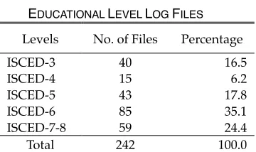
Each line represents a record of the volunteer’s action. The first field represents the virtual key code of the key that the volunteer pressed or released. The second field indicates the date the action took place in the format of yyyy-mm-dd. The third field is the elapsed time since the beginning of that day (12:00 am) in milliseconds, and the forth field is the action, “dn” for key-press and “up” for key-release. We then extracted all the features of keystroke dynamics from the text files. For example, the duration of keystroke is calculated from the sub-traction of ms that correspond to the “up” action minus the ms that correspond to the “dn” action, for the same key. Similarly, all the digram latency representations are calculated. Exam-ples are press-press, press, press-release, and release-release digram latency. The number of log files per educational level is shown in Table 1.
TABLE1
EDUCATIONAL LEVEL LOG FILES
Levels No. of Files Percentage
ISCED-3 40 16.5
ISCED-4 15 6.2
ISCED-5 43 17.8
ISCED-6 85 35.1
ISCED-7-8 59 24.4
Total 242 100.0
The log files varied in size from 170 KB to 271 KB and contained data from 2,800 to 4,500 keystrokes. The class ISCED-2 is absent because there was no log file from a volunteer with this educational level.
There are many useful features that can be extracted from keystroke dynamics. Some of them are temporal, which are usually time-based and measured in millisecond. The most used features in the literature are keystroke duration, which is the time that a key is kept pressed, and the digram latency, which is the time between the pressing or releasing of a key and the pressing or releasing of the next key (this creates four combinations, down-down, down-up, up-down and up-up). In addition, there are other temporal features that have been used or may be used, such as: a) those which include the time associated with the trigrams, tetragrams, etc. [18], b) the num-ber, the duration and the frequency of pauses during typing [19], and c) the typing rate [20].
Except from temporal features, there are non-temporal fea-tures that are non time-based, such as: typing speed (e.g., words per minute), the frequency of errors, error correction mode, finger pressure on the keys [21], which key is used when there are two or more options (e.g., “Shift” [22], “Ctrl”, “Alt”, “Enter”, etc.) [23]. Other non-temporal features may
include the time of day, applications used, and the frequency of using the keyboard.
In this study, we use the most popular features of keystroke dynamics, i.e., keystroke durations and digram latencies. The reason for this is that for keystroke pressure features, a dedi-cated pressure-sensitive keyboard is essential, which contra-dicts with the main advantage of keystroke dynamics biomet-rics. Moreover, the frequency of word errors, typing rate and duplicate keys features are merely practical for text with large number of characters. Finally, trigrams, tetragrams, etc, are much rarer than monograms and digrams [24]. More specifi-cally, we preferred down-down digram latencies (DDDL) to avoid negative values, because the second key may be pressed or may even be released before the releasing of the first key.
The total number of features to consider could have been almost 10,000 if we had used all the keystroke durations and digram latencies assuming an average computer’s keyboard has 100 keys. However, some keys and digrams are used rarely or never. Based on our observation, we decided to in-clude 42 keys and 120 digrams only. To extract features from the log files, we developed “ISqueezeU” software, which reads the text files created by “IRecU” and calculates the aver-age values of durations or latencies. The keys that have at least 10 appearances and the digrams with at least 5 appearances have been taken into account only. The values for the rest keys and digrams were marked as unknown.
The features from our dataset that were used in this work are available on [25].
2.2 Randomised Radial Basis Function Network
[image:4.595.76.256.462.569.2]In this section, we design and modify the radial basis function neural network (RBFN), which was initially proposed by Broomhead and Lowe [26]. RBFN shows faster convergence, smaller extrapolation errors, and higher reliability. It is built on a typical feedforward and three-layered architecture with a single hidden layer, where the activation functions for hidden units are defined as radially symmetric basis functions phi, such as the Gaussian function. Training a RBFN involves two phases: clustering like unsupervised on the hidden layer to de-termine N receptive field centroids in the training data set and the associated widths, and supervised on the output layer to estimate the connection weights w. The output layer is straightforward as it implements a simple multiple linear re-gression using the iterative gradient descent based training method. In each RBF neuron, it is stored a vector with as many dimensions as the number of the input layer neurons. This vector is called “center vector” and is denoted as c. Similarly, the input forms a vector of equal dimensions and the Euclid-ean Distance between the input and the center vector is calcu-lated. The calculated distance is then multiplied by a coeffi-cient b and finally the product is applied to a radial basis func-tion. This procedure is illustrated in Figure 1.
Fig. 1. The structure of the RBF neuron.
[image:4.595.310.552.669.751.2]output of the RBF neuron is given by the outcome of a radial function on the Euclidean distance, i.e.:
(1)
The index in (1) indicates that it is the output of the ith
neu-ron of the network and the double bar denotes the Euclidean distance between vectors. Besides Euclidean distance, Ma-halanobis distance could also be useful as it may give better results in some situations [27]. The radial function produces its largest response when the input vector is equal to the center vector. On the contrary, as the input moves near to the center, the response falls off exponentially as in (2).
(2)
In the third layer, the number of neurons is as many as the number of the categories in which the data will be classified. This means that in our case there are 5 neurons in the output layer. Each output node computes a sort of score for the asso-ciated category. Typically, a classification decision is made by assigning the input to the category with the highest score. The score in every output neuron is computed by taking a weighted sum of the activation values from every RBF neuron, as shown below:
(3)
where N is the number of neurons in hidden layer, a(i) is the
weight assigned to the ith neuron, b(i) is the coefficient of the ith
neuron and c(i) is center vector of the ith neuron. During the
training process, it selects three sets of parameters: the center vectors (c(i)) and beta coefficient (b(i)) for each of the neurons, and
the matrix of output weights between the neurons and the out-put nodes (a(i)). Schwenker et al. [28] provide an overview of
common approaches to training such radial basis based mod-els. In short, they perform the k-Means clustering on their training set and the cluster centers are used as the center vec-tors. The trade off in choosing the number of neurons in hid-den layer is that the more neurons the higher the classifier’s accuracy, while the less neurons the shorter the system’s train-ing time. The average distance between all instances in a clus-ter and the corresponding clusclus-ter cenclus-ter is given by:
(4)
where m is the number of instances belonging to this cluster, xj
is the jth instance in the cluster and C is the cluster center.
Hav-ing the value s, the beta coefficient for the cluster is calculated as:
(5)
The output weights can be trained using the gradient de-scent optimisation technique. The training inputs are the val-ues obtained by the RBF neurons using the training set x. Gra-dient descent runs separately for each output node (that is, for each class in the data set).
Finally, the modified radial basis neural network is ran-domized [29]. A model that does not give satisfactory results we call it “weak”. A strategy to enhance its performance is to combine many “weak learners” (WL) in a way that the output of each classifier can be aggregated to form a final decision. To provide a training set to the next-level classifier, weights are assigned to the instances, which determine the probability that should appear in the next training set. This probability is equal for every instance at the beginning of the procedure and there-fore the first-level classifier uses the entire available training set. Instances with higher weights are more likely to be in-cluded in the next training set, and vice versa. The idea is to increase the weight on the misclassified instances so that these instances will make up a larger part of the next classifiers training set, and hopefully the next trained classifier will per-form better on them. To explain how this works, let assume that there is a binary problem (only two classes) and every kth
instance in the training set has the value pk, while qk is the
cor-rect output after the procedure. Because the problem is binary, the qk may have the values +1 and –1. As mentioned earlier,
weights are assigned to instances of the training set, which are stored to a vector W. Initially, these weights are equal for every instance and therefore all of them participate in the training procedure of the first WL. The weights are adjusted using the equation below:
(6)
where Wt(k) is the weight of the kth instance of the tth classifier
training set, At is a coefficient corresponding to the tth classifier
and indicates its importance to the final result, ft(pk) is the
pre-diction of the tth classifier for the kth instance and St is a
normal-ise factor which ensures that the sum of the instance weights is equal to 1. From the above, it follows that the qk·ft(pk) product
will be positive when the prediction is correct and negative when it is incorrect. Because this product is part of a negative exponent entails that when the prediction is correct the weight of the instance will be decreased and when it is incorrect will be increased. Moreover, the Wt is a distribution because each
weight Wt(k) represents the probability that the kthinstance will
be selected as part of the next training set, and because every weight has value between 0 and 1 and their sum is 1. Once the training of all WL is completed, the output of the final classi-fier is given by:
(7)
where T is the number of WL, ft(p) is the output of the tth WL,
which is +1 or –1 in the case being studied and At is the
coeffi-cient that was assigned to the tth WL. Therefore, the final output
is just a linear combination of all of the WLs and the final de-cision is simply the sign of this sum. It should also be noted that the At coefficients, each of which is computed after the
training of the corresponding classifier as:
(8)
where 𝜀" is the number of misclassifications over the training
set divided by the training set size. According to equation (8),
( )
x
r
(
x
c
)
y
(i)=
-(
)
b x c2e
c
x
r
-
=
- ×-( )
å
= -×
-×
=
N i c x b ie
i ia
x
y
1 ) ( 2 ) ( ) (å
=-×
=
m j jC
x
m
s
11
22
1
s
b
×
=
( )
( )
( ) t p f q A t tS
e
k
W
k
W
t k t k× × -+
×
=
1( )
( )
÷
ø
ö
ç
è
æ
×
=
å
= T t t tf
p
AUTHOR ET AL.: TITLE 5
when the 𝜀" quantity approaches 0 the 𝐴" coefficient grows
ex-ponentially, which means that better classifiers play more im-portant role to the final result. When the 𝜀" quantity is equal to
0.5, i.e., the classifier accuracy is 50%, the 𝐴" is 0 and therefore
every classifier with accuracy no better than random guessing is ignored. Finally, when the 𝜀" is over 0.5, the 𝐴" is negative,
which means that the opposite decision of the classifier is taken into account.
Algorithm 1 summarises the abovementioned operation of R2BN procedure.
The parameters of the Algorithm 2 are the training set x, the “weak learner”, which is the RBFN, and the number of itera-tions T, while n is the training sample size. In each iteration the weighted error ε%, the coefficient At, and the weights Wt are
calculated.
2.3 Data Condensation Method
One of the problems in any classification procedure is that, ir-respective of the sophistication of the classifier in use, as the dataset size increases so does the computational time. As with any other classifier, the training time of R2BN is considerable and highly depends on the number of iterations. One possible solution is to build the classification model on a much smaller representative subset of the original dataset. The aim is to re-duce the dataset size as much as possible with the minimum loss of classifier performance.
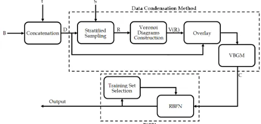
[image:6.595.37.293.606.728.2]To this end, this subsection proposes a new data condensa-tion method, which precedes R2BN as shown in Fig. 2.
Fig. 2. R2BN and data condensation method block diagram. D is stratified
sampled by percentage S and R is produced. Voronoi diagrams V(R) are produced based on R. Dataset D overlies over V(R). VBGM clustering al-gorithm is used to produce dataset C. A number of RBFNs where each one uses different training set, calculated by the previous neural network, performs the classification.
The proposed filter-based random sub-field data condensa-tion method consists of a three stages. In the first stage,
assuming that B is a given training set, with N instances and M features, then the dataset D is a concatenation of B and the target values t. In simple random sampling (SRS), a sample R is selected from B uniformly with replacement following a bi-nomial distribution. Equivalent weights are given to all sam-ples in the dataset, so that any sample is chosen with equal probability regardless of whether it was previously sampled or not [30]. Although SRS simplifies analysis results, it suffers in performance when D is imbalanced, just as it happens in our case, where the class ISCED-4 occupies the 6% of the in-stances and class ISCED-6 the 35%. In the filter-based random sub-field data condensation, D is divided into a set of strata according to the different target values in t, and SRS is per-formed on each stratum independently. In this context, we use the proportional sampling approach, where the proportion sampled from each stratum is equal in the sample as it is in the original dataset. Thus, if D is highly imbalanced, then higher sampling percentage would be given to the small target stra-tum.
Upon sampling from D to produce R, we need to assess whether this sample is a good representative or not. There are two types of statistical tests, namely parametric and nonpara-metric statistical tests. Paranonpara-metric tests make assumptions about the statistical distribution of the original dataset, while non-parametric tests assume no underlying statistical struc-ture about the data. Thus, in order to maintain generality in this framework, the nonparametric preference is adopted.
In this study, the test was performed on the most significant features. The topic of feature subset selection has been well studied in the literature, whereby a feature selection algorithm consists of a search technique in conjunction with an evalua-tion metric. Here, a filter-based feature selecevalua-tion method, which utilises the information gain as an evaluation metric with respect to the class value is used. It can be formalised as:
(9)
where H(x) is the entropy of x, given by
(10)
where E is the length of the vector x and Pr(x[i]) is the proba-bility of the x[i].
The second stage is the construction of a Voronoi diagram V(R) based on the subsampled dataset R. The Voronoi diagram V(R) is the collection of all Voronoi regions VR(rn, R) whose
cen-ters rn are instances in R. For a brief definition of Voronoi
dia-gram let x, yÎÂM. Then the bisector of x and y:
(11)
is the perpendicular line through the center of the line segment 𝑥𝑦
(((. Where 𝐴̅ denotes the closure of some set A and ‖. ‖, is the p-norm distance, defined as:
(12)
The half plane D(x, y) which is separated by the bisector is:
(
class
) (
H
class
Attribute
)
H
IG
=
-
|
( )
x
( )
x
[ ]
i
( )
x
[ ]
i
H
Ei
Pr
ln
Pr
1
å
=
-=
( )
{
M}
p p
y
s
s
s
x
y
x
B
,
=
-
=
-
|
Î
Â
p M
i p i
p
w
w
å
=
=
(13)
and the corresponding Voronoi region of x with respect to R is written as:
(14)
The main method for computing a Voronoi diagram is by the brute force approach. Thus, it could be defined as:
(15)
Variety of efficient algorithms exists to compute the Voronoi diagram, such as the incremental construction, divide & quer, and plane sweep. According to [31], the divide & con-quer algorithm and the plane sweep constructs a Voronoi dia-gram of n points within time O(n·logn) and linear space, in the worst case, where both bounds are optimal.
Here, we used the Euclidean distance measure to calculate the Voronoi regions. Nonetheless, it is worth mentioning that variety of other distance metrics can be chosen depending on the nature of the problem and the data. For example, for con-tinuously-valued attributes, one can employ the Mikowsky, Mahalanobis, Chebychev, Camberra, Quadratic, Correlation, Chi-square, and many others. This stage is very crucial since it re-duces the complexity of the next clustering stage, where we assume that data points that are far apart do not have an effect on each other. As you may have noticed, this approach allows the condensation process performed in parallel to the different Voronoi regions.
In third stage the original dataset D overlies over the Voro-noi diagram V(R). The goal of this stage is to fetch representa-tive centroids from each Voronoi region, for which the collec-tion of all centroids comprise the reduced dataset C. It is re-mained to be decided which clustering algorithm must be used and how many centroids per Voronoi region should be fetched. By specifying as clustering validity measure that the clustering algorithm should attempt to minimise the inter-cluster distance measures and maximise the intra-inter-cluster dis-tance measures, the VBGM clustering algorithm [32] is used to fetch at most -𝑈𝑛/2centroids from each 𝑛"2 Voronoi region,
with 𝑈3 to be the M-dimensional data instances that constitute
the Voronoi region. In this work, α0 is set to 0.01, which most
often results in selecting less than -𝑈𝑛/2. Although, the sam-pling percentage is specified inthe beginning of the algorithm, the final sampling percentage most often ends up being slightly less, where the highest worst case condensation per-centage 𝑃𝐸𝑅78 is
(16)
where 𝐾3 is the number of clusters. The three stages of the
fil-ter-based random sub-field data condensation are described in the following pseudo code.
Algorithm 2 has as parameters the Dataset D and a sam-pling percentage S which takes values between 0 and 1. In stage 1, a representative set R from D is selected by calling a stratified random sampling. The number of selected instances corresponds to the specified parameter S. In stage 2, based on R, a Voronoi diagram V(R) is constructed by partitioning the dataset space into L = 𝑆 × 𝑁 Voronoi regions ÎV(R). Finally, in stage 3, the original instances from D is overlayed back onto V(R) and VBGM clustering algorithm is used to fetch at most -𝑈3/2 centroids from each 𝑛"2Voronoi region. Thus, now it
can be assumed that for each local region in the input space represented by a centre vector and there is corresponding sca-lar output into which it maps then the centroids can be fol-lowed by convolution process as below.
In addition, for datasets of high dimensions, one might em-ploy cheap distance metrics. For instance, only the most sig-nificant features can be chosen for the distance metric, which in turn reduces the time latency of computing the distances drastically. Moreover, one could rely on the construction of an approximate Voronoi diagrams as in the proposed architecture. This stage is very crucial since it reduces the complexity of the next clustering/learning stage. Another note that merits a mention is that this framework allows for parallel condensa-tion to be performed to the different Voronoi regions.
3 M
ODELE
VALUATION ANDA
NALYSISIn this section we evaluate and compare the performances of the proposed R2BN model and other well-known nine machine learning models, namely: i) radial basis function network (RBFN), ii) multi-layer perceptron (MLP), iii) support vector machine (SVM), iv) random forest (RF), v) logistic model tree (LMT), vi) naïve Bayes tree (NBTree), vii) best first tree (BFTree), viii) naïve Bayes (NB) classifier, and ix) simple lo-gistic (SL). The models are tested on the benchmark keystroke dynamics dataset in terms of: a) the model accuracy (Acc.), which is the percentage of correctly classified instances, b) the stability (𝜎), which is the measure of deviation of all the model accuracies over 10-folds, and c) time complexity (TBM), which is the CPU time required to build the model.
More specifically, to assess the performance of the proposed model fairly with regards to the abovementioned criteria (i.e., accuracy, stability, and time complexity), the well-referenced cross-validation is used [33]. In the 10-fold cross-validation, which is the most commonly used version, the dataset is di-vided into 10 subsets. Each time, one of the 10 subsets is used as the testing set and the other 9 subsets are put together to form a training set. Then, the average error across all 10 trials is computed. The advantage of this method is that the way the data gets divided matters less. Every data point gets to be in a testing set exactly once, and in a training set 9 times.
Moreover, to validate the quality of the proposed model,
( )
{
M}
p
p
y
s
s
s
x
y
x
D
,
=
-
<
-
|
Î
Â
( )
!
( )
x y R y
y
x
D
R
x
VR
¹ Î
=
,,
,
(
)
{
M}
p j p n
n
R
r
x
r
x
j
n
x
r
VR
,
=
<
,
"
¹
|
Î
Â
å
=×
-=
Knn n n
wc
U
K
N
PER
AUTHOR ET AL.: TITLE 7
the F-score and ROC index are computed and provided. For the F-score, we calculated the harmonic mean of the specificity and sensitivity [34], where its value falls in the range between 0 and 1. Accuracy is measured by ROC index, the area under the ROC curve [35].
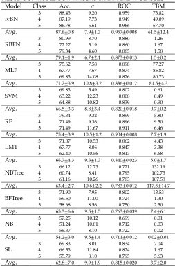
TABLE2
RESULTS OF MODEL COMPARISONS ON DIFFERENT CLASSES Model Class Acc. 𝜎 ROC TBM R2BN
3 88.43 9.20 0.959 73.82
4 87.19 7.73 0.949 49.09
5 86.78 6.61 0.966 67.70
Avg. 87.6±0.8 7.9±1.3 0.957±0.008 61.5±12.4
RBFN
3 80.99 8.70 0.880 1.26
4 77.27 5.19 0.860 1.67
5 79.34 4.60 0.885 1.58
Avg. 79.1±1.9 6.7±2.1 0.873±0.013 1.5±0.2
MLP 3 4 75.62 67.77 7.58 7.67 0.898 0.874 77.27 85.82
5 69.83 14.08 0.876 80.73
Avg. 71.7±3.9 10.8±3.2 0.886±0.012 81.5±4.3
SVM
3 69.83 5.49 0.802 0.61
4 63.22 12.23 0.808 0.49
5 64.88 10.82 0.839 0.90
Avg. 66.5±3.3 8.8±3.4 0.820±0.018 0.7±0.2
RF 3 4 79.34 71.49 9.32 9.36 0.899 0.896 5.80 9.50
5 71.49 11.67 0.911 6.46
Avg. 75.4±3.9 10.5±1.2 0.904±0.008 7.7±1.9
LMT
3 71.07 10.53 0.862 4.43
4 67.77 8.06 0.847 3.38
5 62.40 10.56 0.817 6.68
Avg. 66.7±4.3 9.3±1.3 0.840±0.023 5.0±1.7
NBTree
3 66.12 12.73 0.771 132.19
4 60.74 8.41 0.795 102.73
5 61.16 10.26 0.783 107.58
Avg. 63.4±2.7 10.6±2.2 0.783±0.012 117.5±14.7
BFTree
3 71.90 7.95 0.802 13.53
4 59.50 11.00 0.724 1.30
5 58.68 8.56 0.750 2.50
Avg. 65.3±6.6 9.5±1.5 0.763±0.039 7.4±6.1
NB 3 4 57.25 51.24 10.12 10.81 0.699 0.712 0.01 0.03
5 55.37 8.10 0.722 0.02
Avg. 54.2±3.0 9.5±1.4 0.711±0.012 0.02±0.01
SL
3 69.83 8.01 0.834 2.04
4 66.53 11.84 0.824 1.67
5 55.79 8.10 0.795 5.63
Avg. 62.8±7.0 9.9±1.9 0.815±0.020 3.7±2.0 R2BN (30 clusters for K-Means, 0.9 minimum standard deviation for the clusters and
55 iterations for adaptive boosting, for 5-classes dataset, 30 clusters for K-Means, 1.9 minimum standard deviation for the clusters and 45 iterations for adaptive boosting, for 4-classes dataset, and 60 clusters for K-Means, 1.0 minimum standard deviation for the clusters and 70 iterations for adaptive boosting, for 3-classes dataset), RBFN (70 clusters for K-Means and 1.0 minimum standard deviation for the clusters, for 5-classes dataset, 100 clusters for K-Means and 1.0 minimum standard deviation for the clusters, for 4-classes dataset, and 40 clusters for K-Means and 1.2 minimum standard deviation for the clusters, for 3-classes dataset) MLP (0.7 learning rate and 0.4 momentum, for 5-classes dataset, 0.5 learning rate and 0.6 momentum, for 4-clas-ses dataset, and 0.8 learning rate and 0.6 momentum, for 3-clas4-clas-ses dataset), SVM (1.0 C-value and Polykernel as kernel type, for 5-classes dataset, 1.0 C-value and Polyker-nel as kerPolyker-nel type, for 4-classes dataset, and 3.0 C-value and PolykerPolyker-nel as kerPolyker-nel type, for 3-classes dataset), RF (100 trees with 100 random features each, for 5-classes dataset, 100 trees with 162 random features each, for 4-classes dataset, and 90 trees with 120 random features each, for 3-classes dataset), LMT (10 iterations for LogitBoost, 1 as minimum number of instances for splitting a node and 0.01 beta value for LogitBoost, for 5-classes dataset, 4 iterations for LogitBoost, 1 as minimum number of instances for splitting a node and 0.0 beta value for LogitBoost, for 4-classes dataset, and 10 iterations for LogitBoost, 1 as minimum number of instances for splitting a node, and 0.01 beta value for LogitBoost, for 3-classes dataset), BFTree (5 folds in internal cross validation and 1 as minimum number of instances at the terminal nodes, for 5-classes dataset, 3 folds in internal cross validation and 1 as minimum number of instances at the terminal nodes, for 4-classes dataset, and 30 folds in internal cross validation and 2 as minimum number of instances at the ter-minal nodes, for 3-classes dataset), and SL (no iterations for LogitBoost and 40 as heuristic stop, for 5-classes dataset, 130 iterations for LogitBoost and 50 as heuristic stop, for 4-classes dataset, and no iterations for LogitBoost and 30 as heuristic stop, for 3-classes dataset).
However, as the ISCED-4 class makes only 6.2% of the whole dataset and the learning models rarely see the samples and adjust the weights, increasing the probability of unreliable results (i.e., imbalance effect), ISCED-3 and ISCED-4 classes
are merged forming the new ISCED-3-4 classes. Now the da-taset has the following four classes, i) those who do not have tertiary education, ii) those who have short cycle tertiary edu-cation, iii) those who have university degree, and iv) those who have education higher than tertiary. Again, ISCED-3-4 and ISCED-5 are merged to form a new ISCED-3-4-5 class da-taset. This balances up the number of samples in each class for fair model evaluation and comparisons. The experimental re-sults are summarised in Table 2.
[image:8.595.38.291.152.536.2]R2BN excels all other models in terms of Acc., in 3, 4 and 5-classes datasets, about 8% improved from its base model (RBFN). More specifically, R2BN achieves an accuracy of 86.8% with 5-classes dataset. Similarly, with 4-classes dataset, the dif-ference between the accuracies of the R2BN predictions and the baseline is over 62%, while in 3-classes case this difference is over 54%. In addition, R2BN becomes the second in the stabil-ity behind the RBFN model, achieving 7.9±1.3 deviation of all the model accuracies over 10-folds. Moreover, R2BN has the greatest ROC index, over all other models, reaching a value only 0.043 less than the optimum 1.0 and followed by RF and MLP which have 0.904 and 0.886, respectively. However as our results suggest, almost all the other models require less train-ing time (see Table 2). Specifically, R2BN’s is only better than MLP and NBTree with regards to TBM. It requires considera-bly more time to learn a model than NB (approx. 3075x), SVM (approx. 88x), RBFN (approx. 41x), and RF (approx. 8x).
Fig. 3. Accuracy comparison over three different classes’ datasets.
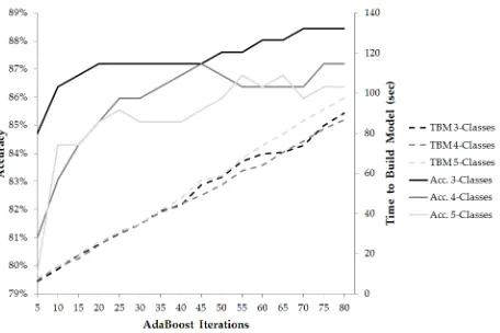
Fig. 3 visualises the experimental results of accuracy for the ten models, over three different datasets. As suggested by our experimental results, randomised radial basis function net-work, seems to be a much more suitable model, achieving 88.43% Acc. We believe that the utility of R2BN can be con-firmed with these experimental results, however, there is a drawback that should be addressed. Specifically, it is obvious that learning an optimal model for R2BN is still time consum-ing. We performed additional experiments on 3, 4, and 5 clas-ses. As shown in Table 3, the weights were converged over 70 iterations, which we believe is causing the issue. Even though the standard RBFN has an advantage of faster convergence, the meta nature of the modified R2BN increases the model complexity leading to slow overall convergence.
As it was expected, the time needed to build the model is increasing linearly as the number of iterations increases, while the accuracy of the system seems to tend to reach a maximum value. This is clearer in Figure 4, which visualises the findings of Table 3.
TABLE3
THE PERFORMANCE OF R2BNMODEL
[image:8.595.312.541.372.519.2]Acc. (%)
TBM (sec)
Acc. (%)
TBM (sec)
Acc. (%)
TBM (sec) 5 84.71 6.09 80.99 6.67 79.75 7.75 10 86.36 12.07 83.06 13.55 84.30 13.71 15 86.78 19.14 84.30 17.53 84.30 19.56 20 87.19 24.56 85.12 24.27 85.12 25.73 25 87.19 29.89 85.95 30.69 85.54 30.54 30 87.19 34.62 85.95 34.62 85.12 34.86 35 87.19 41.17 86.36 40.54 85.12 41.55 40 87.19 44.19 86.78 44.94 85.12 47.55 45 87.19 54.24 87.19 49.09 85.54 56.63 50 87.60 58.22 86.78 54.32 85.95 58.81 55 87.60 66.08 86.36 61.28 86.78 67.70 60 88.02 69.79 86.36 63.82 86.36 73.88 65 88.02 70.54 86.36 70.55 86.78 79.64 70 88.43 73.82 86.36 75.99 85.95 86.08 75 88.43 83.76 87.19 82.16 86.36 91.85 80 88.43 90.13 87.19 86.58 86.36 97.53 The highest accuracy on each dataset is bolded and underlined.
Fig. 4. Accuracy and time needed to build model of different classes’ datasets according the number of iterations.
As seen in Table 3, however, with the configurations of 15 iterations for 3 classes, 25 iterations for 4 classes, and 20 itera-tions for 5 classes, the time complexities could be reduced by 74%, 60% and 62%, respectively which makes the R2BN the most accurate model with time complexity of 24.9±5.8, mean-ing that the time required to build the model is reduced by 60% with less than 2% drop of accuracy.
TABLE4
THE PERFORMANCE OF R2BNMODEL
USING DATA CONDENSATION METHOD
R-Rate
3 Classes 4 Classes 5 Classes Acc.
(%)
TBM (sec)
Acc. (%)
TBM (sec)
Acc. (%)
TBM (sec) 0.0 88.43 73.82 87.19 49.09 86.78 67.70 0.1 81.82 54.68 80.82 40.25 79.09 54.05 0.2 81.68 36.39 78.50 40.76 72.28 50.95 0.3 71.82 29.73 70.62 26.18 73.30 40.12 0.4 77.71 26.28 76.40 23.99 70.66 45.55 0.5 71.14 24.12 66.89 18.64 66.44 32.85 0.6 68.50 19.44 61.72 13.87 57.94 26.68 0.7 63.30 16.21 61.68 11.79 57.28 18.00 0.8 69.51 7.60 56.79 6.97 57.83 15.18 0.9 66.04 5.57 55.36 4.59 59.62 4.76 Results from 0% to 90% condensation.
An alternative way to reduce TBM is the use of a data con-densation method. Table 4 presents the Acc and TBM of R2BN when the data condensation method that was described in
Section 2.4 is used, with sampling percentage from 100% to 10%. As shown by our results, there are instances in which the accuracy of R2BN does not significantly degrade, while TBM reduces remarkably. For example, in 3-classes dataset, when the sampling percentage is 0.4, the model works 3 times faster with a loss of 10% in accuracy.
4 R
ELATED WORKTo the best of our knowledge, we are one of the first to provide a dataset containing keystroke dynamics, which have been collected from free text, recorded from real users during the daily usage of their computer for a long period of time. It also includes demographic data to be used for user classification, such as educational level. The datasets in the literature contain keystroke data, which in most cases, are collected from users typing 2-3 sentences only [36]. Rybnik et al. [37] created a free text dataset, which contains keystrokes from 9 volunteers. Each volunteer typed a long text of more than 250 characters twice in five sessions. Similarly, the dataset of Messerman et al. [38] included keystrokes that were recorded over a 12-month period by 55 volunteers using a web-mail application. Compared to our work, these datasets were created by us-ers' typing in specific environments rather than from normal use. Some other datasets were created on specific devices ra-ther than on the user's device, while the recording was done in a designated area and not in the familiar space (home, of-fice, etc.) of the volunteers. Finally, few datasets were created by long time user recording than in some sessions, and few are those that contain data from thousands of keystrokes in each logfile, as is the case with our own Readers interested in a sur-vey of free text datasets that were created to test user authen-tication methods may refer to Alsultan and Warwick [39].
Regarding to data condensation, because it is a significant procedure in machine learning, especially in cases where the speed of a system is crucial, many methods have been pro-posed to reduce the training time needed. Liu et al. [40] use three different methods to speed up the computation of SVM classifier, namely one with random selection of data and two other using proximity graphs. Similarly, Gamboni et al. [41] aim to increase the speed of SVMs on large datasets using three methods, i.e., blind random sampling and two linear-time methods for guided random sampling. A different ap-proach was proposed by Rizwan and Anderson [42], where an adaptive data condensation scheme for k-NN classifiers is used by reducing the instances in the training data based on the observed similarities.
In most cases, the proposed data condensation methods significantly reduce the computational time with a slight de-crease of the classification performance. The novelty of the proposed method of this paper lies in the possibility of apply-ing to the highly unbalanced datasets, as with the problem we are dealing with.
5 C
ONCLUDINGR
EMARKSKeystroke-based pattern recognition techniques as a tool for behavioural biometrics are of great importance in digital fo-rensics. This paper introduced a novel model which recog-nises and profiles the educational level of an individual who stands behind a keyboard.
[image:9.595.41.269.292.444.2] [image:9.595.34.280.565.747.2]AUTHOR ET AL.: TITLE 9
dwell times and flight times of the participants keystrokes. Recruiting users and capturing their everyday keystroke is a hard task, especially if one considers that keystrokes often contain sensitive information. This increases the complexity of finding participants that can provide real keystroke dynamics and not synthesized ones. While our dataset is limited and affected by our participants’ demographics, to the best of our knowledge, no other dataset with real keystroke dynamics (i.e. one captured from free text) exists. Instead, previous datasets required participants to write free text that was 2-3 sentences long only. By making the features used from our dataset avail-able to the research community, we hope that we will inspire and aid more research in keystroke-based pattern recognition.
In this work, the dataset was fed into a proposed model, named R2BN, which is the randomised modification of a well-known radial basis neural network. R2BN is built on a shallow-learning architecture, which aims to achieve faster conver-gence and smaller extrapolation errors. It improved its perfor-mance in terms of model accuracy, stability, and learning com-plexity. The experimental results on the dynamic keystroke dataset proved that the proposed R2BN can achieve a test error comparable to or better than the state-of-the-art models.
Our experimental results uncovered a limitation of R2BN, namely the long time required to build the model. This can be addressed by either performing fewer iterations on the boost-ing algorithm, or by usboost-ing a new data condensation method. Our evaluation uncovered cases where high accuracy is main-tained while TBM is considerably reduced.
For a given set of keystroke data, the randomisation of ra-dial function based model provides a way of fine-tuning the global model, as well as improving its predictive performance. Having the ability to identify the educational level of a user who types a certain piece of text has significant value in digital forensics. To the best of our knowledge, this study introduces the first model that can achieve above 85% model accuracy, as well as the greatest model stability over three different classes in the keystroke-dynamic-based educational level classifica-tion task. The utility of the proposed model have been proven in dealing with the source of circumstantial evidence for “put-ting fingers on keyboard” and for profiling the characteristics of the users. However, we note that the deployment of such a system must be in accordance with the current, enforced legal and regulatory framework, as the unauthorized analysis of keystrokes entails privacy violations, which might involve sensitive personal information (e.g., in accordance to the EU legislation).
Our plans for future work include further classification tasks such as predicting handedness. We also plan further work on examining alternatives for the data condensation method as a means to reduce the time that is needed to build the R2BN.
R
EFERENCES[1] K. Taha and P. D. Yoo, “SIIMCO: A forensic investigation tool for identifying the influential members of a criminal organization”, IEEE Trans. on Information Forensics & Security, vol. 11, no. 4, pp. 811–822, 2016.
[2] M. Alzaabi, K. Taha, P. D. Yoo and T. A. Martin, “CISRI: A crime in-vestigation system using the relative importance of information spreaders in networks depicting criminals communications”, IEEE Trans. on Information Forensics & Security, vol. 10, no. 10, pp. 2196-2211, 2015.
[3] F. Monrose and A. D. Rubin, “Keystroke dynamics as a biometric for authentication”, Future Generation Computer Systems, vol. 16, pp. 351– 359, 2000.
[4] R. V. Yampolskiy and V. Govindaraju, “Behavioural biometrics: a sur-vey and classification”, Int. J. Biometrics, vol. 1, no. 1, pp. 81-113, 2008. [5] J.X. Yan and L. Yan, “Gender classification of weblog authors”, in 2006
Amer-ican Association for Artificial Intelligence Spring Symposium, 2006, pp. 228-230. [6] A. Mukherjee and B. Liu, “Improving gender classification of blog
authors”, in Proc. 2010 Conf. Empirical Methods in Natural Language Processing, MIT, MA, USA, 2010, pp. 207-217.
[7] N. Cheng, R. Chandramouli and K. Subbalakshmi, “Author gender identification from text”, Digital Investigation, vol. 8, no. 1, pp. 78-88, 2011.
[8] R. Jones, R. Kumar, B. Pang and A. Tomkins, ““I know what you did last summer”: query logs and user privacy”, in Proc. 16th ACM Conf. on Information and Knowledge Management, New York, NY, USA, 2007, pp. 909-914.
[9] F. Rangel, P. Rosso, M. Koppel, E. Stamatatos and G. Inches, “Over-view of the author profiling task at PAN 2013”, notebook for PAN at Conf. and Labs of the Evaluation Forum, Valencia, Spain, 2013. [10] G. Rehm and H. Uszkoreit, The English language in the digital age,
Springer Berlin Heidelberg, 2012.
[11] D. Song, P. Venable and A. Perrig (1997), User recognition by keystroke latency pattern analysis [Online]. Available FTP: http://citese-
erx.ist.psu.edu/viewdoc/down-load?doi=10.1.1.37.7619&rep=rep1&type=pdf.
[12] Y. Zhao, “Learning user keystroke patterns for authentication”, in Proc. World Academy of Science, Engineering and Technology, Vol. 14, Karnataka, India, 2006, pp. 65-70.
[13] K. Hempstalk, “You are what you type?”, in Proc. New Zealand Com-puter Science Research Student Conference, Christchurch, New Zealand, 2008, pp. 24-31.
[14] P. V. P. Sundar and A. V. S. Kumar, “An enhanced disengagement detection in online learning using quasi framework”, Int. J. of Applied Engineering Research, vol. 10, no.55, pp. 1298-1302, 2015.
[15] I. Tsimperidis, S. Rostami and V. Katos, “Age detection through key-stroke dynamics from user authentication failures”, Int. J. of Digital Crime and Forensics, vol. 9, no. 1, pp. 1-16, 2017.
[16] “ISCED: International Standard Classification of Education”, Uis.unesco.org. [Online]. Available: http://www.uis.unesco.org/Ed- ucation/Pages/international-standard-classification-of-educa-tion.aspx.
[17] “IRecU – BU Cyber Security Research Group”, cybersecurity.bourne-mouth.ac.uk. [Online]. Available: https://cybersecurity.bourne-mouth.ac.uk/?page_id=265.
[18] R. Moskovitch, C. Feher, A. Messerman, N. Kirschnick, T. Mustafic, A. Camtepe, B. Löhlein, U. Heister, S. Möller, L. Rokach, and Y. Elo-vici, “Identity theft, computers and behavioral biometrics”, in Proc. 2009 IEEE Int. Conf. on Intelligence and Security Informatics, Pisca-taway, NJ, USA, 2009, pp. 155–160.
[19] A. Goodkind and A. Rosenberg, “Muddying the multiword expres-sion waters: How cognitive demand affects multiword expresexpres-sion production”, in Proc. 2015 Conf. of the North American Chapter of the Association for Computational Linguistics – Human Language Technolo-gies, Denver, CO, USA, 2015, pp. 87-95.
[20] M. Villani, C. Tappert, G. Ngo, J. Simone, H. St. Fort and S.-H. Cha, “Keystroke biometric recognition studies on long-text input under ideal and application-oriented conditions”, in Proc. 2006 Conf. of Com-puter Vision and Pattern Recognition Workshop, New York, NY, USA, 2006, pp. 39.
[21] H. Saevanee and P. Bhattarakosol, “Authenticating user using key-stroke dynamics and finger pressure”, in Proc. 6th IEEE Conf. on Con-sumer Communications and Networking, Piscataway, NJ, USA, 2009, pp. 1078-1079.
[22] N. Bartlow and B. Cukic, “Evaluating the reliability of credential hard-ening through keystroke dynamics”, in Proc. 17th Int. Symposium on Software Reliability Engineering, Raleigh, NC, USA, 2006, pp. 117-126. [23] A. Kumar, A. Patwari and S. Sabale, “User authentication by typing
Research in Computer and Communication Engineering, vol. 3, no. 10, pp. 8132-8134, 2014.
[24] P. S. Teh, S. Yue and A. B. J. Teoh, “Feature fusion approach on key-stroke dynamics efficiency enhancement”, Int. J. of Cyber-Security and Digital Forensics, vol. 1, no. 1, pp. 20-31, 2012.
[25] “Keystroke dynamics datasets – BU Cyber Security Research Group”, cy-bersecurity.bournemouth.ac.uk. [Online]. Available:
https://cybersecurity.bournemouth.ac.uk/?page_id=624.
[26] D. S. Broomhead and D. Lowe, “Multivariable functional interpolation and adaptive networks”, Complex Systems, vol. 2, pp. 321-355, 1988.
[27] A. G. Bors and I. Pitas, “Median radial basis functions neural net-work”, IEEE Trans. on Neural Networks, vol. 7, no. 6, pp. 1351-1364, 1996.
[28] F. Schwenker, H. A. Kestler and G. Palm, “Three learning phases for radial-basis-function networks”, Neural Networks, vol. 14, no. 4-5, pp. 439-458, 2001.
[29] O. Y. Al-Jarrah, O. Alhussein, P. D. Yoo, S. Muhaidat, K. Taha and K. Kim, “Data randomization and cluster-based partitioning for botnet intrusion detection”, IEEE Trans. on Cybernetics, vol. 46, no. 8, pp. 1796-1806, 2016. [30] K. Josien, M. C. Liu, T. W. Liao, and E. Triantaphyllou, “An evaluation of
sampling methods for data mining with fuzzy C-means” in Data mining for design and manufacturing, Norwell, MA, USA: Kluwer Academic Publish-ers, 2001, pp. 355-369.
[31] F. Aurenhammer and R. Klein, “Voronoi diagrams”, in Handbook of computational geometry, chapter V: Elsevier Science Publishing, 2000, pp. 201-290.
[32] C. Bishop, Pattern recognition and machine learning. New York: Springer, 2006.
[33] P. Refaeilzadeh, L. Tang and H. Liu, “Cross-validation”, in Encyclopedia of Database Systems. New York: Springer, 2009, pp. 532-538, 2009.
[34] N. Ye, K. M. A. Chai, W. S. Lee and H. L. Chieu, “Optimizing F-measures: A tale of two approaches”, in Proc. 29th Int. Conf. Machine Learning, Edin-burgh, U.K., 2012, pp. 289-296.
[35] D. M. W. Powers, “Evaluation: From precision, recall and F-measure to ROC, informedness, markedness and correlation”, J. Machine Learning Technologies, vol. 2, no. 1, pp. 37-63, 2011.
[36] E. Vural, J. Huang, D. Hou, S. Schuckers, “Shared research dataset to sup-port development of keystroke authentication”, in Proc. IEEE International Joint Conference on Biometrics, Clearwater, FL, USA, 2014, pp. 1-8. [37] M. Rybnik, M. Tabedzki, M. Adamski and K. Saeed, “An exploration of
keystroke dynamics authentication using non-fixed text of various length”, in Proc. 2013 Int. Conf. on Biometrics and Kansei Engineering, Tokyo, Japan, 2013. pp. 245-250.
[38] A. Messerman, T. Mustafic, S. A. Camtepe and S. Albayrak, “Continuous and Non-intrusive Identity Verification in Real-time Environments based on Free-Text Keystroke Dynamics”, in Proc. 2011 Int. Joint Conf. on Biomet-rics, Washington, DC, USA, 2011, pp. 1-8.
[39] A. Alsultan and K. Warwick, “Keystroke dynamics authentication: A sur-vey of free-text methods”, Int. J. of Computer Science Issues, vol. 10, issue 4, no. 1, pp. 1-10, 2013.X. Liu, J. F. Beltran, N. Mohanchandra and G. T. Tous-saint, “On speeding up support vector machines: Proximity graphs versus random sampling for pre-selection condensation”, Int. J. of Computer and Information Technology, vol. 7, no. 1, pp. 133-140, 2013.
[40] X. Liu, J. F. Beltran, N. Mohanchandra and G. T. Toussaint, “On speeding up support vector machines: Proximity graphs versus random sampling for pre-selection condensation”, Int. J. of Computer and Information Technol-ogy, vol. 7, no. 1, pp. 133-140, 2013.
[41] M. Gamboni, A. Garg, O. Grishin, S. M. Oh, F. Sowani, A. Spalvieri-Kruse, G. T. Toussaint and L. Zhang, “An empirical comparison of support vector machines versus nearest neighbour methods for machine learning applica-tions”, in Proc. Int. Conf. on Pattern Recognition Applications and Methods, An-gers, France, 2014, pp. 110-129.