Audio video based Segmentation and Classification using SVM and AANN

Audio-video based Segmentation and Classification

using SVM and AANN

K. Subashini

Research Scholar

Department of Computer Science and Engineering Annamalai University,Annamalainagar-608 002, India

S. Palanivel

Professor

Department of Computer Science and Engineering Annamalai University,Annamalainagar-608 002, India

V. Ramaligam

Professor

Department of Computer Science and Engineering Annamalai University,Annamalainagar-608 002, India

ABSTRACT

In this paper, we propose a method for combining audio and video for segmentation and classification. The objective of seg-mentation is to detect the category change point such news to advertisement. The classification system classify the audio-video data into one of the predefined categories such as news, adver-tisement, sports, serial and movies. Mel frequency cepstral co-efficients(MFCC) are used as acoustic features and color his-togram is used as visual features for segmentation and classifi-cation. Support vector machine(SVM) and autoassociative neu-ral network(AANN) models are used for segmentation and clas-sification. The evidence from audio and video are combined us-ing weighted sum rule for both segmentation and classifications.

General Terms:

Audio-video segmentation, Audio-video classification

Keywords:

Support vector machines(SVM),Auto associative neural net-work(AANN),Mel frequency cepstral coefficients,Color his-togram,Audio and video segmentation,Audio and video classi-fication,Weighted sum rule

1. INTRODUCTION

In this era of growing information technology, the information is flooding in the form of audio, video, text and audiovisual. Real time broadcasters as well as commercial broadcasters are enabled with devices to easily broadcast and store multimedia contents. This data, Once broadcast and stored, are not changed for any case. Manual handling of this data is impractical for real-time campaigning applications because of its increasingly large volume. Hence, it is important to have a method of automati-cally index multimedia data for targeting and commercial broad casting application based on multimedia contents. Segmentation and classification of data into different categories is one impor-tant step for building such systems. Our main objective in this paper is combining individual results audio-video segmentation and classification. Audio and video detection and categorization are emerging research area.

1.1 Related work

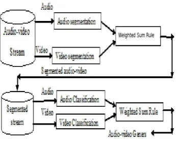
classifica-Fig. 1. Combining audio and video segmentation and classification

tion and annotation algorithm is obtained. Then, in[26] a survey on visual content based video indexing and retrieval shows huge information on video. In [31] a high-accurancy audio classifica-tion algorithm is proposed based on SVM-UBM using MFCCs as classification features. A effective algorithm for unsupervised speaker segmentation using AANN is described in [10]. In [1] a robust speaker change detection algorithm is proposed. Evalua-tion of classificaEvalua-tion techniques for audio indexing is described in[3]. In [5] a hybride approach is presented for audio segmen-tation. Acoustic, strategies for automatic segmentation are de-scribed in[12]. In [16] unsupervised speaker change detection using SVM missclassification rate is described. Automatic seg-mentation, classification and clustering of broadcast news audio is given in [21].

1.2 Outline of the work

In this paper, audio and video are combined for segmentation and classification. Fig. 1., Shows the block diagram of audio and video segmentation and classification. The paper is organized as follows: Acoustic feature extraction and Visual feature extrac-tion are described in Secextrac-tion 2. Modeling techniques used for segmentation and classification are described in Section 3. Seg-mentation and classification methods are in Section 4., and 5, respectively. Experimental results are explained in section 6. Fi-nally, conclusions is given in section 7.

2. FEATURE EXTRACTION FOR

SEGMENTATION AND CLASSIFICATION

2.1 Acoustic Feature Extraction

MFCC is perceptually motivated representation defined as the cepstrum of a windowed short-time signal. A non-linear mel-frequency scale is used which approximates the behaviour of the auditory system. The MFCC is based on the extraction of the sig-nal energy with-in critical frequency bands by means of a series of triangular filters as shown in Fig. 2. Whose centre frequencies are spaced according to melscale. The mel-cepstrum exploits auditory principles as well as the decorrelating property of the cepstrum [10]. Fig. 3. illustrates the computation of MFCC fea-tures for a segment of audio signal which is described as follows : The mel-frequency cepstrum has proven to be highly effec-tive in recognizing structure of music signals and in modeling the subjective pitch and frequency content of audio signals. Psy-chophysical studies have found the phenomena of the mel pitch

Fig. 2. Mel scale filter bank

Fig. 3. Extraction of MFCC from audio signal

scale and the critical band, and the frequency scale-warping to the mel scale has led to the cepstrum domain representation. The mel scale is defined as

Fmel=

clog 1 +f c

log(2) (1)

whereFmelis the logarithmic scale offnormal frequency scale.

The mel-cepstral features, can be illustrated by the MFCCs, which are computed from the fast Fourier transform (FFT) power coefficients. The power coefficients are filtered by a triangular bandpass filter bank. Whenc in (1) is in the range of 250 -350, the number of triangular filters that fall in the frequency range 200 - 1200 Hz (i.e.,the frequency range of dominant au-dio information) is higher than the other values of c. There-fore, it is efficient to set the value ofc in that range for cal-culating MFCCs.Denoting the output of the filter bank bySk

(k= 1,2,· · ·, K), the MFCCs are calculated as cn=

r 2 K

K

X

k=1

(logSk) cos

h

n(k−0.5) π K i

, n= 1,2· · ·, L

Fig. 4. An example of a Feature Extraction. (a) Input Image. (b) Color Histogram.

Fig. 5. Principle of Support Vector Machine.

2.2 Visual Feature Extraction

A color histogram is a representation about distribution of colors in a representation about distibution of colors in an image, de-rived by counting the number of pixels in each of the given set of color ranges in a typically two dimensional(2D) color space. A histogram of an image is produced first by dicretization of the colors in the image into a number of bins, and counting the num-ber of image pixels in each bin. The histogram provides a com-pact summarization of the distribution of data in a image. The color histogram of an image is relatively invariant with trans-action and rotation about the viewing axis, and may vary very slowly with the view angle. Further, they are computationally trivial to compute. Moreover, small changes in camera viewpoint has on color histograms. Hence, they are used to compare images in many applications. This work uses color histogram as visual feature. The RGB color space is quantized into64bins by n.64 bin histogram extracted from an image is shown Fig. 4.

3. MODELING TECHNIQUES USED FOR

SEGMENTATION AND CLASSIFICATION

3.1 Support Vector Machine (SVM)

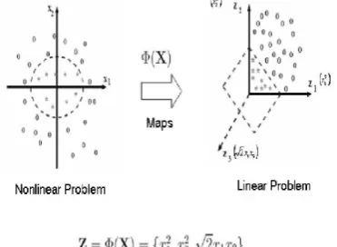
The SVM method is based on structural risk minimization prin-ciple and finds the best balance between the model complexity and learning ability according to the limited sample of informa-tion. The basic idea is to find the optimal separable hyper-plane that not only spearates the two classes without error, but makes the largest interval between them. SVM transforms input vec-tors into a high-dimensional feature space using a non-linear transformationφ, and then to do a linear separation in feature space as shown in Fig. 5. Support Vector Machine (SVM) can be used for classifying the obtained data (Burges, 1998). SVMs are a set of related supervised learning methods used for classi-fication and regression. They belong to a family of generalized linear classifiers. Let us denote a feature vector (termed as pat-tern) byx=(x1, x2,· · ·, xn)and its class label byysuch that

y = {+1,−1}. Therefore, consider the problem of separating the set ofn-training patterns belonging to two classes

(xi, yi), xi∈Rn, y={+1,−1}, i= 1,2,· · ·, n

A decision functiong(x)that can correctly classify an input pat-ternxthat is not necessarilly from the training set. A linear SVM is used to classify data sets which are linearly separable. The SVM linear classifier tries to maximize the margin between the separating hyperplane. The patterns lying on the maximal mar-gins are called support vectors. Such a hyperplane with maxi-mum margin is called maximaxi-mum margin hyperplane [24]. In case of linear SVM, the discriminant function is of the form:

g(x) =wt_{x+b (3)}

such thatg(xi)≥0foryi= +1andg(xi)<0foryi=−1.

In other words, training samples from the two different classes are separated by the hyperplaneg(x) = wt_{x+b = 0. SVM}

finds the hyperplane that causes the largest separation between the decision function values from the two classes. Now the total width between two margins is _w2tw, which is to be maximized.

Mathematically, this hyperplane can be found by minimizing the following cost function:

J(w) =1 2w

t_w

(4) Subject to separability constraints

g(xi)≥+1 for yi= +1

or

g(xi)≤ −1 for yi=−1

Equivalently, these constraints can be rewritten more compactly as

yi wtxi+b

≥1; i= 1,2,· · ·, n (5)

For the linearly separable case, the decision rules defined by an optimal hyperplane separating the binary decision classes are given in the following equation in terms of the support vectors:

Y =sign

i=Ns

X

i=1

yiαi(xxi) +b

!

(6) whereY is the outcome, yi is the class value of the training

example andxirepresents the inner product. The vector

corre-sponds to an input and the vectorsxi, i= 1, . . . , Ns, are the

sup-port vectors. In Eq. 6,bandαiare parameters that determine the

hyperplane. A non-linear support vector classifier implementing the optimal separating hyperplane in the feature space with a ker-nel function K(xi,xnew) is given by

f(xnew) =sgn SV

X

i=1

αiyiK(xi, xnew) +b

! (7) The SVM has two layers. During the learning process, the first layer selects the basisK(xi, xnew),i = 1,2,· · ·, N, from the

given set of bases defined by the kernel; the second layer con-structs a linear function in this space. This is completely equiv-alent to constructing the optimal hyperplane in the correspond-ing feature space. The SVM algorithm can construct a variety of learning machines by use of different kernel functions. Three kinds of kernel functions are usually used. They are

(1) Polynomial kernel of degreed

K(x1, x2) = (γhx1, x2i+c0)

d

(8) (2) Gaussian radial basis function (RBF)

K(x1, x2) =exp −γkx1−x2k2

Input layer Layer

.

.

.

.

.

.

.

.

.

.

.

.

.

.

.

Compression layer

Output layer 1

2

3

4

5

Fig. 6. A Five Layer AANN Model.

(3) Sigmoidal kernel

K(x1, x2) = tanh (γhx1, x2i+c0) (10)

where kernel parameters

—γ: width of RBF coefficient in polynomial —d: degree of polynomial

—c0: additive constant in polynomial

3.2 Autoassociate Neural Network (AANN)

Autoassociative neural network models are feedforward neural networks performing an identity mapping. The modality would be the ablity to solve the scaling problem. The AANN is used to capture the distribution of the input data and learning rule in[19],[29]. Let us consider the five layer AANN model shown in Fig. 6, which has three hidden layers. The processing units in the first and third hidden layers are non-linear, and the units in the second compression/hidden layer can be linear or non-linear. As the error between the actual and the desired output vectors is minimized, the cluster of points in the input space determines the shape of the hypersurface obtained by the projection onto the lower dimensional space. A five layer autoassociative

neu-ral network model is used to capture the distribution of the fea-ture vectors. The second and fourth layers of the network have more units than the input layer. The third layer has fewer units than the first or fifth. The activation functions at the second, third and fourth layers are non-linear. The non-linear output function for each unit istanh(s), Wheresis the activation value of the unit. The standard backpropagation learning algorithm is used to adjust the weights of the network to minimize the mean square error for each feature vector. The AANN captures the distribu-tion of the input data depending on the constraints imposed by the structure of the network, just as the number of mixtures and Gaussian functions do in the case of Gaussian mixture model. Gaussian mixture model.

4. AUDIO VIDEO SEGMENTATION

4.1 Audio and Video Segmentation using SVM

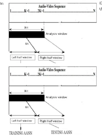
The proposed audi(video) segmentation uses a sliding window of about 2 sec assuming the category change point occurs in the middle of the window. The sliding window is intially placed at the left end of the audio(video) signal. The SVM is trained to

Fig. 7. SVM Based Segmentation Algorithm.

Fig. 8. AANN Based Segmentation Algorithm.

classify the feature vectors in the left half of the window, and the feature vectors in the right half of the window and it is shown in Fig. 7. The SVM is tested with all these feature vectors. a

low missclassification or a high correct classification indicated a category change point such as news to advertisement because the SVM is able to discriminate the two classes. SVM training and testing are repeated by moving the window with a shift of 80 msec until it reaches the right end of audio(video) signal.

4.2 Audio and Video Segmentation using AANN

The proposed audi(video) segmentation uses a sliding window of about 2 sec assuming the category change point occurs in the middle of the window. The sliding window is intially placed at the left end of the audio(video) signal. The AANN model is trained to capture the distribution of the feature vectors in the left half of the window, and the feature vectores in the right half of the window are used for testing as shown in Fig. 8. The out put of the model is compared with the input to compute the nar-malized squared error (ei) for theithfeature vector (yi) is given

by,

ek=

kxi−oik2

kxik2

(11) whereoiis the output vector given by the model. The errorekis

transformed into a confidence scoresusing

s= exp(−ek) (12)

4.3 Combining Audio-Video Segmentation

The evidence from audio and video segmentation from SVM(AANN) are combined using weighted sum rule. The weighted sum rule states that ”‘If the category change point is detected att1 from the audio and att2 is within a threshold t

then the category change point is fixed att1+t2 2 ”.

5. AUDIO AND VIDEO CLASSIFICATION

5.1 Audio-Video Classification using SVM

Support vector machine is trained to distingush acoustic(visual) features of a category from all other categories. One svm is cre-ated for each category. For testing, acoustic(visual) features are given as input to the svm model and the distance between each of the feture vectors and the svm hyperplane is optained. The aver-age distance is calculated for each model. The category of audio is decided based on the maximum distance.

5.2 Audio and Video Classification using AANN

Autoassociative neural network is used to capture the distribu-tion of the acoustic(visual) feature vectors of a category. Separate AANN model are trained to capture the distribution of acous-tic(visual) feature vectors of each category. For testing, each acoustic(visual) feature vector is given as input to each of the models. The output of the model is compared with the input to compute the normalized squared error. The normalized squared error is transfered into a confidence score as described in section 6.1. The average confidence score is calculated for each model. The category is described based on highest confidence score.

5.3 Combining Audio-video Classification using SVM

The evidence from audio and video classifications are combined using weighted sum rule. The audio and video classification re-sults obtained by SVM are combined using:

mj=

w naj+

1−w

p vj,1≤j≤c, (13) Where

aj= i=1

X

n

xj

i (14)

vj= i=1

X

p

yj

i (15)

xji=

1, if ca i =j

0, otherwise (16)

yj_i =

1, if cv i =j

0, otherwise (17) ca

i =Category label forithaudio frame.

cv

i =Category lable forithvideo frame.

vj= video based score forjthcategory.

aj= audio based score forjthcategory.

mj= Combined audio and video based score forjthcategory.

c= number of category. n= number of audio frames. p= number of video frames. w= weights.

The category is decided based on the highestmj.

Fig. 9. Audio-Video Based Segmentation Using AANN.

Similarly, the results obtained for audio and video classification by AANN are combined using:

s=w n

n

X

i=1

sa i +

(1−w) p

p

X

i=1

sv

i (18)

nis the number of frames in audio signal. pis the number of frames in video signal. sa

i is the confidence score rate of theithaudio frame.

sv

i is the confidence score of theithvideo frame.

sis the combined audio and video confidence score. wis weight.

The category is decided based on the highest confidence score obtained from the models.

6. EXPERIMENTAL RESULTS

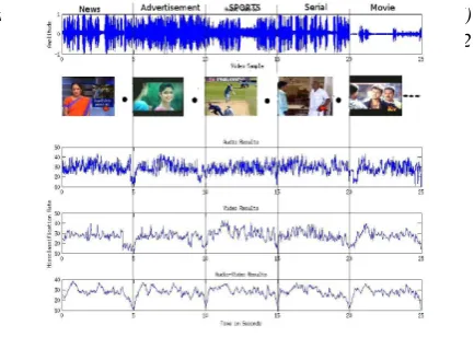
In order to test the performance of the proposed audio-video segmentation and classification system is evaluated using the TV broadcasting programs audio-video collections from various channels, comprising different durations of audio-video ranging from five seconds to one hour.The recording consits news fol-lowed by sports etc. In our work, the audio sequence should be cut into short audio segments. Multi-channel audio signals are pre sampled across multiple inputs, they are downsampling rate of 8000khz and 16 bit monophonic PCM formate. For each au-dio clip, features described above is extracted every 20ms, with a 30 ms overlap. This section analyzes the performance of the pro-posed audio-video classification in two phases. Initially, the in-dividual segmentation of the audio and video genre are used for classification and the combined results are evaluated. For con-ducting experiments, video data is recorded using a TV tuner card at 25frames/s,240*320 pixels size of images from various television channels at different timings to ensure variety of data. All the geners are collected from various channels from differ-ent regional language channels.The first phase, individual frames of the audio and video genre are used for the experiments. For segmenting visual and acoustic are obtained for all the training and testing frames. Then, weighted sum rule matching is used to find the distance between two segmentations as described in Section 4. The sample segmentation using SVM and AANN are shown in 9,. and 10., respectively. The overall segmentation performance is reported in 11. For combining the audio,video

and audio-video optained shifting the frames 4:1 ratio of audio and video frames used through out the experiment. In our work the analysing frame is set as 2 sec data set for both audio and video. The performance of the method is compared with audio

Fig. 10. Audio-Video Based Segmentation Using SVM.

Fig. 11. Performance Diagram of Audio-Video Segmentation Based on SVM and AANN.

Fig. 12. Performance diagram of Audio-Video Based Classification using SVM and AANN.

and 1. The sample performance for classification is reported in 12.

7. CONCLUSIONS

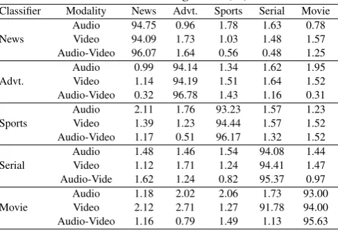
In this paper, a method was proposed for combining audio and video data for segmentation and classification. In this work mel-frequency cepstral coefficients and color-histogram are used as

Table 1. Performance of proposed algorithm for audio-video classification using AANN(%)

Classifier Modality News Advt. Sports Serial Movie Audio 94.75 0.96 1.78 1.63 0.78 News Video 94.09 1.73 1.03 1.48 1.57 Audio-Video 96.07 1.64 0.56 0.48 1.25 Audio 0.99 94.14 1.34 1.62 1.95 Advt. Video 1.14 94.19 1.51 1.64 1.52 Audio-Video 0.32 96.78 1.43 1.16 0.31 Audio 2.11 1.76 93.23 1.57 1.23 Sports Video 1.39 1.23 94.44 1.57 1.52 Audio-Video 1.17 0.51 96.17 1.32 1.52 Audio 1.48 1.46 1.54 94.08 1.44 Serial Video 1.12 1.71 1.24 94.41 1.47 Audio-Vide 1.62 1.24 0.82 95.37 0.97 Audio 1.18 2.02 2.06 1.73 93.00 Movie Video 2.12 2.71 1.27 91.78 94.00 Audio-Video 1.16 0.79 1.49 1.13 95.63

Table 2. Performance of proposed algorithm for audio-video classification using SVM(%)

Classifier Modality News Advertisement Sports Serial Movie

Audio 97.4 078 0.0 0.0 1.82

Advt. Video 97.96 1.38 0.44 0.0 0.22

Audio-Video 99.04 0.64 0.0 0.0 0.32

Audio 1.42 96.09 0.50 0.50 1.49

News Video 0.78 96.22 0.0 1.15 1.85

Audio-Video 0.62 98.18 0.0 0.64 0.86

Audio 2.08 0.96 95.48 0.0 1.48

Sports Video 1.98 1.09 96.46 0.47 0.0

Audio-Video 0.58 0.38 99.04 0.0 0.0

Audio 1.73 2.87 0.0 94.9 0.5

Serial Video 0.86 1.47 0.0 96.28 1.39

Audio-Vide 0.54 0.87 0.0 97.99 0.60

Audio 1.17 1.02 0.0 1.03 96.78

Movie Video 0.92 0.78 0.86 0.66 96.78

Audio-Video 0.30 0.70 0.0 0.68 98.52

8. REFERENCES

[1] J. Ajmera, I. McCowan, and H. Bourland. Robust speaker change detection.IEEE Journal of Signal Process Letter, 11(8):649–651, Aug 2004.

[2] J. Ajmera, I. McCowan, and H. Bourlard. Speech/music segmentation using entropy and dynamism features in a HMM classification framework. Speech Communication, 40(3):351–363, 2003.

[3] J. A. Arias, J. Pinquier, and R. Ande-Obrecht. Evaluation of classification techniques for audio indexing.In proc. 13th Eropean conf. Signal Processing, 2005.

[4] Drain Brezeale and Diane J.Cook. Automatic video clas-sification a survey of the literature.IEEE Transaction on System,Man,and cybernetic, 38(3):416–430, May 2008. [5] S. Cheng and H. Wang. Metric SEQDAC: A hybrid

ap-proach for audio segmentation. Proc. 8th International conference on spoken language Process., pages 1617– 1620, Oct 2004.

[6] Zhouyu Fu, Guojun Lu, Kai Ming Ting, and Dengsheng Zhang. A survey of audio-based music classification and annotation. IEEE Transactions Multimedia, 13(2):303– 318, April 2011.

[7] M.Kalaiselvi Geetha, S.Palanivel, and V.Ramaligam. A novel block intensity code for video classification and re-trieval. Expert System With Applications, 36:6415–6420, 2009.

[8] W.J. Gillespie and D.T. Nguyen. Video classification using a tree-based RBF network.IEEE International Conferance on image processing, 3(1):465–468, 2005.

[9] R. Jarina, M. Paralici, M. Kuba, J. Olajec, A. Lukan, and M. Dzurek. Development of reference platform for generic audio classification development of reference plat from for generic audio classification.IEEE Computer society, Work shop on Image Analysis for Multimedia Interactive,, pages 239–242, 2008.

[10] S. Jothilaskmi, S. Palanivel, and V. Ramalingam. Unsuper-vised speaker segmentation with residual phase and MFCC features.Expert System With Applications, 36:9799–9804, 2009.

[11] K. Kaabneh, A. Abdullah, and A. Al-Halalemah. Video classification using normalized information distance. In Proceedings of the geometric modelling and imaging-new trends, pages 34–40, 2005.

[12] T. Kemp, M. Schmidt, M. Westphal, and A. Waibel. Acous-tic strategies for automaAcous-tic segmentation of audio data. Proc. IEEE International conference on Acoust, Speech, Signal Process., pages 1423–1426, jun 2000.

[13] Serkan Kiranyaz, Ahmad Farooq Qureshi, and Moncef Gabbouj. A generic audio classification and segmenta-tion approach for multimedia indexing and retrieval.IEEE Trans. Audio, Speech and Lang Processing, 14(3):1062– 1081, May 2006.

[14] J. Kittler, M. Hatef, R.P. Duin, and J.Matas. On com-bining classifier.IEEE Trans. Pattern Anal. Mach. Intell., 20(3):226–239, 1998.

[15] C. Lin, J. Shih, K. Yn, and H. Lin. Automatic music genre classification based on modulation spectral analysis of spectral and cepstral features.IEEE Transactions Multi-media, 11(4):670–682, June 2009.

[16] P.C. Lin, J.C. Wang, J.F. Wang, and H.C. Sung. Unsuper-vised speaker change detection using SVM training mis-classsification rate.IEEE Int’l Conf. Acoustics, Speech and Signal Processing, 14(3):1062–1081, May 2006.

[17] Lie Lu, Hong-Jiang Zhang, and Stan Z. Li. Content-based audio classification and segmentation by using support vec-tor machines.Springer-Verlag Multimedia Systems, 8:482– 492, 2003.

[18] Yu-Fei. Ma and Hong-Jiang. Zhang. Motion pattern based video classification using support vector machines.In Pro-ceedings of IEEE International Symposium on Circuit and Systems, 2:69–72, 2002.

[19] S. Palanivel.Person Authentication using Speech, Face and Visual Speech. Ph.D thesis, Indian Institute of Technology Madras, Department of Computer Science and Engg, 2004. [20] P.Dhanalakshimi, S.Palanivel, and V.Ramaligam. Classifi-cation of audio signals using SVM and RBFNN.Expert System With Applications, 36:6069–6075, 2009.

[21] M. Sieglar, U. Jain, B. Raj, and R. Stern. Automatic seg-mentation, classification and clustering of broadcast news audio.Proc. DARPA Speech recognition workshop, pages 97–99, 1997.

[22] V. Suresh, C. Krishna Mohan, R. Kumaraswamy, and B. Yegnanarayana. Content-based video classification us-ing SVM.In International conference on neural informa-tion processing, 2004.

[23] V. Suresh, C. Krishna Mohan, R. Kumaraswamy, and B. Yegnanarayana. Combining multiple evidence for video classification. In IEEE internationalconference intelli-gent sensing and information processing, pages 187–192, jan2005 2005.

[24] V. Vapnik. Statistical Learning Theory. John Wiley and Sons, New York, 1998.

[25] Y. Wang, Z. Liu, and J.C. Huang. Multimedia content anal-ysis using both audio and visual clues.IEEE Signal Pro-cess. Mag., 17:12–36, 2000.

[26] H. V. Weiming, Nianhua xie, Li. Li, Xiang Lin Zeng, and Stephen maybank. A survey on visual content-based video indexing and retrival. IEEE Transaction on Sys-tem,Man,and cybernetic, part c:1–23, 2011.

[27] L. Xu, A. Krzyzak, and C.Y. Suen. Methods of combining multiple classifiers and their applications to handwriting recognition.IEEE Trans. Syst. Man, Cybern., 2:418–435, 1992.

[28] L. Q. Xu and Y. Li. Video classification using spactial-temporal features and PCA.International Conference on Multimedia and Expo, 3:345–348, 2003.

[29] B. Yegnanarayana and S.P. Kishore. AANN: An alterna-tive to GMM for pattern recognition.Neural Networks, 15, 2002.

[30] Y. Yuan and C. Wan. The application of edge features in au-tomatic sports genre classification.In Proceedings of IEEE Conference on Cybernetics and Intelligent Systems, pages 1133–1136, 2004.