Numerical Study of Free Convection Flow Past
a Vertical Cone with Variable Heat and Mass Flux
S. Gouse Mohiddin
Department of Mathematics,Madanapalle Institute of Technology & Science, Madanapalle, AP, India
O. Anwar Bég
Mechanical Engineering Subject Group, Sheffield Hallam University, Sheffield,S1 1WB, England, UK
S. Vijaya Kumar Varma
Department of Mathematics, Sri Venkateswara University,Tirupati - 517502, AP, India
ABSTRACT
A numerical study of buoyancy-driven unsteady natural convection boundary layer flow past a vertical cone embedded in a non-Darcian isotropic porous regime with transverse magnetic field applied normal to the surface is considered. The heat and mass flux at the surface of the cone is modeled as a power-law according to
q x
w( )
x
m and*
( )
nw
q x
x
respectively, where x denotes the coordinate along the slant face of the cone. Both Darcian drag and Forchheimer quadratic porous impedance are incorporated into the two-dimensional viscous flow model. The transient boundary layer equations are then non-dimensionalized and solved by the Crank-Nicolson implicit difference method. The velocity, temperature and concentration fields have been studied for the effect of Grashof number, Darcy number, Forchheimer number, Prandtl number, surface heat flux power-law exponent (m), surface mass flux power-law exponent (n), Schmidt number, buoyancy ratio parameter and semi-vertical angle of the cone. Present results for selected variables for the purely fluid regime are compared with the published work and are found to be in excellent agreement. The local skin friction, Nusselt number and Sherwood number are also analyzed graphically. The study finds important applications in geophysical heat transfer, industrial manufacturing processes and hybrid solar energy systems.Keywords
Cone; Free convection, Magnetohydrodynamic (MHD) flow, non-Darcian porous media; finite difference method; heat mass flux;
1.
NOMENCLATURE
x, y coordinates along the cone generator and normal to the generator
u,v velocity components along the x- and y-directions g gravitational acceleration
r
local radius of conet
timet dimensionless time
T
temperatureT dimensionless temperature
C
concentrationC dimensionless concentration D mass diffusion coefficient K permeability of porous medium
w
q
heat flux (i.e. heat transfer rate per unit area)
*
w
q
mass flux (i.e. mass transfer rate per unit area) k thermal conductivity of fluid
L reference length
X, Y dimensionless coordinates along the cone generator and normal to the generator
U,V dimensionless velocity components along the X- and Y-directions
b Forchheimer geometrical constant Da Darcy number
Fs Forchheimer number GrL Grashof number
M magnetic parameter B0 magnetic field strength
Pr Prandtl number
N buoyancy ratio parameter Sc Schmidt number
m power-law index for surface heat flux relation n power-law index for surface mass flux relation Nux local Nusselt number
NuX dimensionless local Nusselt number
Shx local Sherwood number
ShX non-dimensional local Sherwood number
R dimensionless local radius of cone Greek symbols
dynamic viscosity of fluid kinematic viscosity of fluid semi-vertical cone angle thermal diffusivity
volumetric thermal expansion coefficient dimensionless temperature function dimensionless time
X dimensionless local shear stress function (skin friction)
Subscripts
w
condition on the wall∞ free stream condition
2.
INTRODUCTION
Darcy law. However, for high velocity flow situations, the Darcy law is inapplicable, since it does not account for inertial effects in the porous medium. Such flows can arise for example in the near-wellbore region of high capacity gas and condensate petroleum reservoirs and also in highly porous filtration systems under high blowing rates. The most popular approach for simulating high-velocity transport in porous media is the Darcy–Forchheimer drag force model. This adds a second-order (quadratic) drag force to the momentum transport equation. This term is related to the geometrical features of the porous medium and is independent of viscosity. Vafai and Tien [5] presented a seminal study discussing the influence of Forchheimer inertial effects in porous media convection. Chen and Chen [6] studied the mixed convective boundary layer flow from a vertical surface in a fluid-saturated non-Darcian porous medium including Forchheimer inertial effects. Hossain and Paul [7] studied thermal convection boundary layer flow with buoyancy and suction/blowing effects from a cone with non-uniform surface temperature. They extended this study [8] to consider non-uniform surface heat flux, both studies employing numerical methods. Chamkha et al. [9] studied the double-diffusive convection heat and mass transfer over a cone (and wedge) in Darcy-Forchheimer porous media. Magnetohydrodynamic (MHD) flow and heat transfer is of considerable interest because it can occur in many geothermal, geophysical, technological, and engineering applications such as nuclear reactors and others. The geothermal gases are electrically conducting and are affected by the presence of a magnetic field. Vajravelu and Nayfeh[10] studied hydromagnetic convection from a cone and a wedge with variable surface temperature and internal heat generation or absorption. Thusfar the transient thermal convection flow over a cone in Darcy-Forchheimer porous media has not been studied in the literature despite important applications in geothermics, geophysics and materials processing.
3.
MATHEMATICAL MODEL
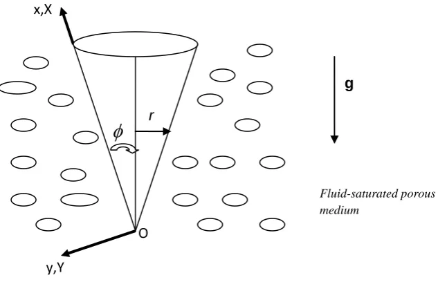
An axisymmetric unsteady natural convection boundary layer flow past a vertical cone with transverse magnetic field applied normal to the surface with variable heat and mass flux in a Darcy-Forchheimer fluid saturated porous medium in a cartesian (x, y) coordinate system is formulated mathematically in this section. Initially, it is assumed that the cone surface and the surrounding fluid which are at rest possess the same temperatureT and concentration levelC everywhere in the fluid. At time t 0, heat supplied from the cone surface to the fluid, concentration level near the cone surface are raised at a rate of qw
x xmand
* n
qw x x respectively, and they are maintained at the same level. It is assumed that the concentration Cof the diffusing species in the binary mixture is very less in comparison to the other chemical species, which are present and hence the Soret and Dufour effects are negligible. We consider viscous flow where pressure work, viscous dissipation and thermal dispersion effects are neglected. The coordinate system chosen (as shown in Fig.1) is such that the x-direction is measured along the cone surface from the leading edge O, and the y-direction is normal to the cone generator. The cone apex is located at the origin(x=y=0). Here designates the semi-vertical angle of the cone and r is
the local radius of the cone. Then under the above assumptions, the governing boundary layer equations with Boussinesq’s approximation are
0 ur vr x y (1)
2 2
0 cos ( )
2
* 2
cos ( )
B
u u u u
u v u g T T
t x y y
b
g C C u u
K K (2) 2 2
T T T T
u v
t x y y
(3)
2 2
C C C C
u v D
t x y y
(4)
where all terms are defined in the nomenclature. Under the Boussinesq approximation buoyancy effects are simulated only in the momentum equation, which is coupled to the energy equation, constituting a free convection regime. The corresponding spatial and temporal initial and boundary conditions at the surface and far from the cone take the form:
0 : 0, 0, ,
t u v TT C Cfor all x, y
*
( ) ( )
0 : 0, 0, T qw x , C qw x
t u v
y k y D
at y = 0
0, ,
u T T C Cat x = 0, (5) u0,TT ,CC as
y
. where all the parameters defined in the nomenclature.The equations (1) to (4) are highly coupled, parabolic and nonlinear. An analytical solution is clearly intractable and in order to facilitate a numerical solution we non-dimensionalize the model. Proceeding with the analysis we now introduce the following transformations: x X L ,
1 4 y Y GrL L , R r
L
, where rxsin,
41 vL V GrL ,
1 2 uL U GrL ,
1 2 2 t t GrL L 2 2 1
0 2 B L M GrL
(6)
0
UR VR
X Y
(7)
2
2 cos cos
2
U U U U Fs
U V MU T NC U
X Y Y DaGrL Da
U
t
(8)2 1
2 Pr
T T T T
U V
t X Y Y
(9)
2 1
2
C C C C
U V
t X Y Sc Y
(10)
The corresponding non-dimensional initial and boundary conditions are given by
0 : 0, 0, 0, 0
t U V T C for all X, Y,
0 : 0, 0, T m, C n
t U V X X
Y Y
at Y = 0, (11)
0
U , T 0, C0 at X = 0, 0,
U T0, C0 as Y .
Where again all the parameters are given in the nomenclature. The dimensionless local values of the skin friction, Nusselt number and the Sherwood number are given by the following expressions
0 U x
Y Y
(12)0 T
Nux X
Y Y
(13)0 C
Shx X
Y Y
(14)4.
NUMERICAL SOLUTION
In order to solve the unsteady, non-linear, coupled equations (7) – (10) under the conditions (11), an implicit finite difference scheme of Crank-Nicolson type has been employed which is discussed by many authors Muthucumaraswamy and Ganesan [11], Gouse Mohiddin [12] and Gouse Mohiddin et al [13] and Bapuji et al. [14]. The finite difference scheme of dimensionless governing equations is reduced to tri-diagonal system of equations and is solved by Thomas algorithm as discussed in Carnahan et al. [15]. The region of integration is considered as a rectangle with
1 max
X and Ymax 22 where Ymaxcorresponds to Y which lies very well out side both the momentum and thermal boundary layers. The maximum of Y was chosen as 22, after some preliminary investigation so that the last two boundary conditions of (11) are satisfied within the tolerance limit105. The mesh sizes have been fixed as X 0.05,
0.05 Y
with time step t 0.01. The computations are carried out first by reducing the spatial mesh sizes by 50% in one direction, and later in both directions by 50%. The results are compared. It is observed in all cases, that the results differ only in the fifth decimal place. Hence, the choice of the mesh sizes seems to be appropriate. The scheme is unconditionally stable. The local truncation error is O( t2 Y2 X)and it tends to zero as t, X and Ytend to zero. Hence, the scheme is compatible. Stability and compatibility ensure the convergence. The derivatives involved in Equations (12) – (14) are evaluated using five point approximation formula.
5.
RESULTS AND DISCUSSION
[image:4.595.77.257.381.522.2]
Fig 1: Physical Model
Table 1 Comparison of local skin friction values at X = 1.0 and m = 0.5 with those of Hossain-Paul [8] for steady state
purely fluid (Da in present model) case.
Pr
Hossain and Paul
[8] X/GrL
3/5
Present results
0.01
5.13457 5.13424
0.05
2.93993 2.93180
0.1
[image:4.595.69.276.560.696.2]2.29051 2.29044
Table 2 Comparison of local Nusselt number values at X = 1.0 and m = 0.5 with those of Hossain-Paul [8] for steady
state purely fluid (Da in present model) case.
Pr
Hossain and Paul [8]
NuX/GrL 3/5
Present results
0.01
0.14633 0.14648
0.05
0.26212 0.26227
0.1
0.33174 0.33648
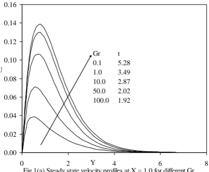
In Figures 1(a) and 1(b), the influence of Grashof number (
l
Gr
) on steady state velocity(U) and temperature (T) distributions with Y-coordinate are shown. Free convection i.e. thermal buoyancy effects are analyzed via the Grashof number. For an increasingGr
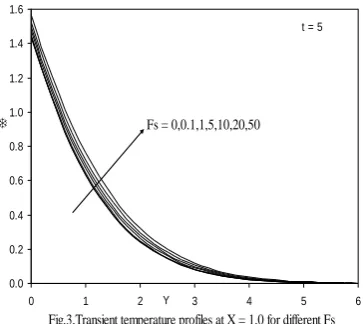
l from 0.1 through 1.0, 10.0,50.0 to 100.0 cooling of the cone by free convection occurs i.e. heat is conducted away from the cone to the surrounding regime. Figures 2(a) and 2(b) show the effect of Darcy number (Da) on dimensionless velocity (U) and temperature (T) with transformed radial coordinate (Y) close to the leading edge (i.e. cone apex) at X = 1.0. To study the influence of regime permeability from sparsely packed media to densely packed materials the following values Da = 1.0, 0.1, 0.01, 0.001 are considered. Da = K L2for a fixed value of the reference length (L) is directly proportional to permeability (K) of the porous regime. Increasing Da increases the porous medium permeability and simultaneously decreases the Darcian impedance since progressively less solid fibers are present in the regime. The flow is therefore accelerated for higher Da values causing an increase in the velocity U as shown in Figure 2(a). Maximum effect of rising Darcy number is observed at intermediate distance from the cone surface around Y 1. Conversely temperature T depicted in Figure 2(b) is opposed by increasing Darcy number. The presence of fewer solid fibers in the regime with increasing Da inhibits the thermal conduction in the medium which reduces distribution of thermal energy. The regime is therefore cooled when more fluid ispresent and T values in the thermal boundary layer are decreased. Profiles for both velocity and temperature are smoothly asymptotic decays to the free stream indicating that excellent convergence (and stability) is obtained with the numerical method. Velocity boundary layer thickness will be increased with a rise in Da and thermal boundary layer thickness reduced. The effect of the Forchheimer inertial drag parameter (Fs) on dimensionless temperature (T) profiles is shown in Figure 3. The Forchheimer drag force is a second order retarding force simulated in the momentum conservation equation. Increasing Fs values from 0.0 through 0.1,1.0,5.0,10.0,20.0 and 50.0 causes a strong increase in Forchheimer drag which
g
y,Y
x,X
O
r
decelerates the flow i.e. reduces velocities. For higher values of Fs it is expected that the porous medium flow becomes increasingly chaotic. Temperature (T) however is slightly increased with a rise in Forchheimer parameter. The effects of the Prandtl number (Pr) on velocity profiles are depicted in Figure 4. Pr encapsulates the ratio of momentum diffusivity to thermal diffusivity. Larger Pr values imply a thinner thermal boundary layer thickness and more uniform temperature distributions across the boundary layer. Hence thermal boundary layer will be much less thick than the hydrodynamic (translational velocity) boundary layer. Smaller Pr fluids have higher thermal conductivities, so that heat can diffuse away from the cone surface faster than for higher Pr fluids (thicker boundary layers). Physically the lower values of Pr correspond to liquid metals (Pr 0.02, 0.05), Pr = 0.7 is accurate for air or hydrogen and Pr = 7.0 for water. The computations show that translational velocity U is therefore reduced as Pr rises from 0.72 through 1.0, 2.0, 5.0, 7.0 and 10.0 since the fluid is increasingly viscous as Pr rises. Figure 4(b) indicates that a rise in Pr substantially reduces the temperature T in saturated porous regime. The profiles become increasingly parabolic as Pr increases above 0.1, for which the profile is approximately a linear decay. For all cases T decays to zero as Y , i.e. in the free stream. There is however a rapid decay to zero for the maximum Pr (= 10) where the temperature plummets to zero in the near-wall region. Concentration function values are seen to increase slightly with an increase in Pr.
Figure 5 shows the effect of the Schmidt number (Sc) on the dimensionless concentration (C). We note that the Schmidt number (Sc) embodies the ratio of the momentum to the mass diffusivity. Sc therefore quantifies the relative effectiveness of momentum and mass transport by diffusion in the hydrodynamic (velocity) and concentration (species) boundary layers. Smaller Sc values can represent for example hydrogen gas as the species diffusing in air , Sc = 2.0 implies hydrocarbon diffusing in air, and higher values to petroleum derivatives diffusing in fluids (e.g. ethyl benzene) as indicated by Gebhart et al. [16]. As Sc increases, Figure 5 shows that C values are strongly decreased, as larger values of Sc correspond to a decrease in the chemical molecular diffusing i.e. less diffusion therefore takes place by mass transport. The dimensionless concentration profiles all decay from a maximum concentration to zero in the freestream. Greater Sc values correspond to lower chemical molecular diffusivity of the parent fluid so that less diffusion of the species occurs in the regime. Concentration boundary layer thickness will therefore be reduced. For low Sc fluid greater species diffusion occurs and concentration boundary layer thickness increased. For Sc = 1, the Concentration and velocity boundary layers will have approximately the same thickness i.e. species and momentum will be diffused at the same rates. With lower Sc values the decay of concentration from the cone surface is more controlled, for increasing values of Sc the profiles descend more and more steeply and concentration falls faster from the surface to a short distance into the boundary layer regime.The effect of surface heat flux power
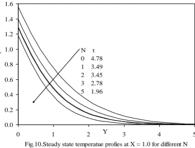
exponent (m) on the steady state temperature (T) is shown in Figure 6. An increase in the value of m reduces the temperature. It is also seen that the time required to reach the steady state temperature is more at lower values of m. Figure 7 depict the distribution of concentration (C) with radial coordinate (Y) for various values of the surface mass flux power law exponent (n). The concentration reduces with the increasing n values from 0.0 through 0.25, 0.50, 0.75 and 1.0. Increasing Fs clearly reduces the local Nusselt number as shown in Figure 8. A slight increase in local Nusselt number accompanies the increment in Pr as shown in Figure 9. The influence of the concentration to thermal buoyancy ratio parameter (N), on dimensionless temperature (T) with radial coordinate (Y) is shown in Figure 10. N = 0 indicates that thermal and species buoyancy forces are both absent. For N > 0, thermal and species buoyancy forces aid each other. N = 1 implies that both buoyancy forces are of the same order of magnitude. A rise in N from 0.0 through 1.0, 2.0, 3.0 and 5.0 induces a retarding effect on the flow in the porous regime i.e. velocities are decreased. Increasing N (thermal and concentration buoyancy forces assisting each other) decreases temperatures in the regime i.e. cools the boundary layer regime. The effect of semi-vertical angle of the cone () on dimensionless temperature (T) with Y-coordinate is shown in Figure 11. It is observed that a rise in substantially increases the temperature T in the boundary layer regime. And more time is required to reach the steady state. Figures 12 the influence of magnetic parameter (M) versus spanwise spatial distributions of velocity U are depicted. Application of magnetic field normal to the flow of an electrically conducting fluid gives rise to a resistive force that acts in the direction opposite to that of the flow. This force is called the Lorentz force. This resistive force tends to slow down the motion of the fluid along the cone and causes an increase in its temperature and a decrease in velocity as M increases. An increase in M from 1 though 2, 3, 4 clearly reduces streamwise velocity U both in the near-wall regime and far-field regime of the boundary layer.
0.00 0.02 0.04 0.06 0.08 0.10 0.12 0.14 0.16
0 2 4 6 8
Gr t 0.1 5.28 1.0 3.49 10.0 2.87 50.0 2.02 100.0 1.92 U
Y
0.0 0.2 0.4 0.6 0.8 1.0 1.2 1.4 1.6
0 2 4 6
T
Y
Fig.1(b).Steady state temperature profiles at X = 1.0 for different Gr Gr t
0.1 5.28 1.0 3.49 10.0 2.87 50.0 2.02 100.0 1.92
0.00 0.02 0.04 0.06 0.08 0.10 0.12 0.14 0.16 0.18
0 2 4 6 8
U
Y
Fig.2(a).Transient velocity profiles at X = 1.0 for different Da Da = 0.001,0.01,0.1,1
t = 5
0.0 0.2 0.4 0.6 0.8 1.0 1.2 1.4 1.6 1.8
0 1 2 3 4 5 6 7
Da = 0.001,0.01,0.1,1 T
Y
Fig.2(b).Transient temperature profiles at X = 1.0 for different Da
t = 5
0.0 0.2 0.4 0.6 0.8 1.0 1.2 1.4 1.6
0 1 2 3 4 5 6
Fs = 0,0.1,1,5,10,20,50
T
[image:6.595.321.503.75.237.2]Y
Fig.3.Transient temperature profiles at X = 1.0 for different Fs
t = 5
0.00 0.02 0.04 0.06 0.08 0.10 0.12 0.14 0.16 0.18 0.20
0 2 4 6 8 10 12
Pr t 0.72 6.73 1 3.36 2 3.19 5 3.22 7 3.49 10 11.13 U
Y
Fig.4. Steady state velocity profiles at X=1.0 for different Pr
0.0 0.2 0.4 0.6 0.8 1.0 1.2 1.4 1.6 1.8 2.0
0 1 2 3 4 5 6
Sc t 0.1 1.99 0.5 2.71 1.0 3.58 3.0 4.02 5.0 4.88 C
Y
6.
REFERENCES
[1] Ingham, D. B., Pop, I. 2002. Transport Phenomena in Porous Media II, Pergamon, Oxford.
[2] Nield, D. A., Bejan, A. 2006. Convection in Porous Media, 3rd edition, Springer, New York.
[3] Vafai, K. (Ed.). 2005. Handbook of Porous Media, 2nd edition, CRC Press, Boca Raton.
[4] Trevisan, O. V., Bejan, A. 1990. Combined heat and mass transfer by natural convection in a porous medium, Adv. Heat Transfer, 20 (1990) 315-352.
0.0 0.2 0.4 0.6 0.8 1.0 1.2 1.4 1.6 1.8
0 1 2 3 4 5
m t 0.00 3.52 0.25 3.52 0.50 3.49 0.75 3.46 1.00 3.44 T
Y
Fig.6.Steady state temperature profiles at X = 1.0 for different m
0.0 0.2 0.4 0.6 0.8 1.0 1.2
0.0 0.5 1.0 1.5 2.0 2.5 n t
[image:7.595.96.278.72.405.2]0.00 3.08 0.25 3.06 0.50 3.49 0.75 3.88 1.00 4.17
Fig.7.Steady state concentration profiles at X = 1.0 for different n C
Y
0.0 0.1 0.2 0.3 0.4 0.5 0.6 0.7 0.8
0.0 0.2 0.4 0.6 0.8 1.0 1.2 Fs = 0,0.1,1,5,10,20,50
X
Fig.8.Effect of Fs on local Nusselt number at X = 1.0
Nu
X
t = 5
0.0 0.1 0.2 0.3 0.4 0.5 0.6 0.7 0.8 0.9
0.0 0.2 0.4 0.6 X 0.8 1.0 1.2
Fig.9.Effect of Pr on local Nusselt number at X = 1.0
Nu
X
Pr t 0.72 6.73 1 3.36 2 3.19 5 3.22 7 3.49 10 11.13
0.0 0.2 0.4 0.6 0.8 1.0 1.2 1.4 1.6
0 1 2 3 4 5
[image:7.595.327.526.76.227.2]N t 0 4.78 1 3.49 2 3.45 3 2.78 5 1.96 T
Fig.10.Steady state temperatue profies at X = 1.0 for different N Y
0.0 0.5 1.0 1.5 2.0 2.5
0 2 4 6 8 10
t 20 3.49 30 8.49 55 11.24
Fig.11. Steady state temperature profiles at X=1.0 for different
T
Y
0.0 0.1 0.2 0.3 0.4 0.5 0.6 0.7 0.8 0.9 1.0
0 2 4 6 8 10
M t 1 4.21 2 5.44 3 6.59 4 7.63 U
[image:7.595.87.530.79.746.2] [image:7.595.323.524.272.602.2]Y
[5] Vafai, K., Tien, C. L. 1981. Boundary and inertia effects on flow and heat transfer in porous media, Int. J. Heat Mass Transfer, 24 (1981)195-203.
[6] Chen, C. H., Chen, C. K. 1990. Non-Darcian mixed convection along a vertical plate embedded in a porous medium, Applied Mathematical Modelling, 14 (1990) 482-488.
[7] Hossain, M.A., Paul, S.C. 2001. Free convection from a vertical permeable cone with non-uniform surface temperature, Acta Mechanica, 151 (2001) 103-114. [8] Hossain, M.A., Paul, S.C. 2001. Free convection from a
vertical permeable circular cone with non-uniform surface heat flux, Heat Mass Transfer, 37 (2001) 167-173.
[9] Chamkha, A.J., Khalid, A. R. A., Al-Hawaj, O. 2000. Simultaneous Heat and Mass Transfer by Natural Convection from a Cone and a Wedge in Porous Media, J. Porous Media, 3 (2000) 155-164.
[10]Vajravelu, K., Nayfeh, L. 1992. Hydromagnetic convection at a cone and a wedge, Int Commun Heat Mass Transfer, 19 (1992) 701–710.
[11]Muthucumaraswamy, R., Ganesan, P. 1998. Unsteady flow past an impulsively started vertical plate with heat and mass transfer, Heat Mass Transf., 34 (1998) 187-193.
[12]Gouse Mohiddin, S. 2011. Computational Fluid Dynamics, LAP Lambert Academic Publishing, Germany.
[13]Gouse Mohiddin, S., Prasad, V. R., Varma, S. V. K., Anwar Bég, O. 2010. Numerical Study Of Unsteady Free Convective Heat And Mass Transfer In A Walters-B Viscoelastic Flow Along A Vertical Cone, Int. J. of Appl. Math. and Mech., 6 (2010) 88-114.
[14]Bapuji Pullepu, Ekambavanan, K., Chamkha, A. J. 2008. Unsteady laminar free convection from a vertical cone with uniform surface heat flux, Nonlinear Analysis: Modelling and Control., 13 (2008) 47-60.
[15]Carnahan, B., Luther, H. A., Wilkes, J.O. 1969. Applied Numerical Methods, John Wiley and Sons, New York. [16]Gebhart, B., Jaluria, Y., Mahajan, R.L., Sammakia, B.
1998. Buoyancy – Induced flows and Transport,