Application of Soft Computing Methods for Economic Load Dispatch Problems

(1)

Application of Soft Computing Methods for Economic

Load Dispatch Problems

Hardiansyah

Department of Electrical Engineering Tanjungpura University Pontianak 78124, Indonesia.

Junaidi

Yohannes MS

ABSTRACT

Economic load dispatch problem is an optimization problem where objective function is highly non linear, non-convex, non differentiable and may have multiple local minima. Therefore, classical optimization methods may not converge or get trapped to any local minima. This paper presents a comparative study of three different evolutionary algorithms i.e. differential evolution, artificial bee colony algorithm and particle swarm optimization for solving the economic load dispatch problem. All the methods are tested on 3-units and 6-units test system. Simulation results are presented to show the comparative performance of these methods.

Keywords

Economic Load Dispatch, Differential Evolution, Artificial Bee Colony, Particle Swarm Optimization.

1. INTRODUCTION

Economic load dispatch (ELD) is defined as the process of allocating generation levels to the generating unit in the mix, so that the system load is supplied entirely and most economically. The objective of an ELD problem in power system operation is to determine the optimal combination of power outputs for all generators, which minimizes the total fuel cost while satisfying constraints [1]. In the traditional ELD problem, the cost function for each generator is approximately represented by a single quadratic function and the problem is solved using mathematical programming based on optimization techniques such as the lambda-iteration, gradient and dynamic programming methods. However, many mathematical assumptions such as convexity, quadratic, differentiable or linear objectives are required to simplify the problem [2].

Several classical optimization techniques need derivative information of the objective function to determine the search direction. But actual fuel cost functions are linear, non-convex, non differentiable and may have multiple local minima [3]. Recently some heuristic techniques such as genetic algorithm [4], ant colony search algorithm [5], evolutionary programming [6], improved tabu search [7], differential evolution [8], particle swarm optimization [9] and artificial bee colony algorithm [10] have been used to solve the complex non-linear optimization problem.

In this paper ELD problem has been solved using three different evolutionary algorithms i.e. differential evolution (DE), artificial bee colony (ABC) algorithm and particle swarm optimization (PSO). Performance of each algorithm for solving the ELD problem has been investigated and simulation results are presented in terms of accuracy, reliability and execution time.

The rest of this paper is organized as follow. Section 2 presents the ELD formulation. Section 3 presents evolutionary algorithm. Results and discussions are given in section 4, and section 5 gives some conclusions.

2. ECONOMIC LOAD DISPATCH

FORMULATION

The objective of an ELD problem is to find the optimal combination of power generations that minimizes the total generation cost while satisfying an equality constraint and inequality constraints. The fuel cost curve for any unit is assumed to be approximated by segments of quadratic functions of the active power output of the generator. For a given power system network, the problem may be described as optimization (minimization) of total fuel cost as defined by (1) under a set of operating constraints.







 





n

i

i i i i i n

i i

T

F

P

a

P

b

P

c

F

1 2

1

)

(

(1)

where

F

_Tis total fuel cost of generation in the system ($/hr), ai, bi, and ci are the cost coefficient of the i th generator, Pi is

the power generated by the i th unit and n is the number of generators.

The cost is minimized subjected to the following generator capacities and active power balance constraints.

n

i

P

i,min



i



i,max

for



1 ,

2 ,



,

(2)

where Pi, min and Pi, max are the minimum and maximum power

output of the i th unit.

Loss n

i i

D

P







1

(3)

where PD is the total power demand and PLoss is total

transmission losses.

The transmission losses PLoss can be calculated by using B

matrix technique and is defined by (4) as,

j ij n

i n

j i

Loss

P

B

P



 



1 1

(4)

(2)

3. EVOLUTIONARY ALGORITHM

3.1 Differential Evolution (DE)

Differential evolution (DE) is a population based evolutionary algorithm, capable of handling non-differentiable, non-linear and multi-modal objective functions [11-13]. A brief description of different steps of DE algorithm is given below:

3.1.1. Initialization

The population is initialized by randomly generating individuals within the boundary constraints





D

j

N

i

X

rand

X

p

j j

j ij

,

2 ,

1 ;

,

2 ,

1 *

max min

min 0











(5)

where

X

_ij0is the initialized jth decision variable of ith population set; ‘rand’ function generates random values uniformly in the interval [0,1]; Np is the size of the population; D is the number of decision variables. The fitness function is evaluated for each individual.

X

min_j and

X

max_j are the lower and upper bound of the jth decision variable, respectively.

3.1.2. Mutation

As a step of generating offspring, the operations of ‘mutation’ are applied. ‘Mutation’ occupies quite an important role in the reproduction cycle. The mutation operation creates mutant vectors

X

_i'kby perturbing a randomly selected vector

X

_ak with the difference of two other randomly selected vectors

k b

X

and

X

_ck at kth iteration as per following equation.





p

k c k b k

a k i

N

i

X

Fx

X

,

2 ,

1

'











(6)

where

X

_i'kis the newly generated ith population set after performing mutation operation at kthiteration;

X

_ak,

X

_bk and

k c

X

are randomly chosen vectors at kth iteration

)

,

2 ,

1 (





N

_p



and

a



b



c



i

.

X

_ak,

X

_bk and

k c

X

are selected for each new parent vector.

]

2 ,

0 [



Fx

is known as ‘scaling factor’ used to control the amount of perturbation in the mutation process and improve convergence. Many schemes of creation of a candidate are possible.

Here strategy 1 has been mentioned in the algorithm.

3.1.3. Crossover

Crossover represents a typical case of a ‘genes’ exchange. The parent vector is mixed with the mutated vector to create a trial vector, according to the following equation:













otherwise

X

q

j

or

Cr

j

rand

if

X

k i

k ij k i

'

" ₍₇₎

where i=1,2,…, Np ; j=1, …, D. k

ij k

ij

X

,

'

,

and

" are the jth individual of ith target vector, mutant vector, and trial

vector at kth iteration, respectively. q is a randomly chosen index  (j = 1,2, …, D) that guarantees that the trial vector gets at least one parameter from the mutant vector even if Cr =0. Cr = [0, 1] is the ‘Crossover constant’ that controls the diversity of the population and aids thealgorithm to escape from local optima.

3.1.4. Selection

Selection procedure is used among the set of trial vector and the updated target vector to choose the best. Each solution in the population has the same chance of being selected as parents. Selection is realized by comparing the objective function values of target vector and trial vector. For minimization problem, if the trial vector has better value of the objective function, then it replaces the updated one as per following equation.















otherwise

X

f

X

if

X

k i

k i k

i k i k

i

)

(

" " 1

(8)

where

X

_ik1 is the ith population set obtained after selection operation at the end of kth iteration, to be used as parent population set (in ith row of population matrix) in next iteration (k + 1th).

3.2 Artificial Bee Colony (ABC)

Artificial Bee Colony (ABC) is one of the most recently defined algorithms by Dervis Karaboga [14, 15]. It has been developed by simulating the intelligent behavior of honey bees. In ABC system, artificial bees fly around in a multidimensional search space and the employed bees choose food sources depending on the experience of themselves. The onlooker bees choose food sources based on their nest mates experience and adjust their positions. Scout bees fly and choose the food sources randomly without using experience. Each food source chosen represents a possible solution to the problem under consideration. The nectar amount of the food source represents the quality or fitness of the solution. The number of employed bees or the onlooker bees is equal to the number of food sources or possible solutions in the population. A randomly distributed initial population is generated and then the population of solutions is subjected to repeated cycles of the search process of the employed bees, onlookers and scouts. An employed bee or onlooker probabilistically produces a modification on the position in her memory to find a new food source (solution) and evaluates the nectar amount (fitness) of the new food source. If the nectar amount of the new food source is higher than that of the previous one then the bee remembers the new position and forgets the old one. Once the employed bees complete their search process, they share the nectar information of the food sources and their position information with the onlooker bees on the dance area. The onlooker bees evaluate the nectar information and choose a food source depending on the probability value associated with that food source using (9).





e

N

j j i i

fit

P

1

(9)

where fiti is the fitness value of the solution i which is

(3)

onlookers produce a modification in the position selected by it using (10) and evaluate the nectar amount of the new source.

v

_ij



x

_ij





_ij



x

_ij



x

_kj



(10) where k



{1, 2,…., ne} and j



{1, 2, …,D} are randomly

chosen indexes. Although k is determined randomly, it has to be different from i.



_ij is a random number between [-1, 1]. It controls the production of neighborhood food sources. If the nectar amount of the new source is higher than that of the previous one, the onlookers remember the new position; otherwise, it retains the old one. In other words, greedy selection method is employed as the selection operation between old and new food sources.

If a predetermined number of trials do not improve a solution representing a food source, then that food source is abandoned and the employed bee associated with that food source becomes a scout. The number of trials for releasing a food source is equal to the value of ‘limit’, which is an important control parameter of ABC algorithm. The limit value usually varies from 0.001NeD to NeD. If the abandoned source is xij, j



(1, 2,..., D)then the scout discovers a new food source xij

using (11).

x

_ij



x

_j_min



rand

(

0 ,

1 )





x

_j_max



x

_j_min



(11)

Where

x

_j_minand

x

_j_maxare the minimum and maximum limits of the parameter to be optimized. There are four control parameters used in ABC algorithm. They are the number of employed bees, number of unemployed or onlooker bees, the limit value and the colony size. Thus, ABC system combines local search carried out by employed and onlooker bees, and global search managed by onlookers and scouts, attempting to balance exploration and exploitation process [15].

The algorithmic steps involved in ABC algorithm are as follows:

1) Generate n random solutions with in boundaries of the system

P



P

_min



rand



(

P

_max



P

_min

)

2) Calculate the objective function and fitness of each solution

3) Store the best fit as Pbest solution

4) A mutant solution is formed using a randomly selected neighbour,

P

_k_mu_tan_t



P

_k

(

i

)





P

_j

(

i

)



P

_k

(

i

)







2 

rand



1 

Where j is the randomly selected neighbour and i is a random parameter

5) Replace

P

_k_mu_tan_tby

P

_k, if the mutant has higher fitness or lower fuel cost of generation.

6) Repeat the above procedure for all the solutions 7) Probability of each solution is calculated as Probability (i) =a*fitness (i)/max (fitness) + b Where {a+b =1}

8) The solution P is selected if its Probability is greater than a random number,

If (rand<probability (i))

Solution is accepted for mutation Else

Go for next solution

Counter is Incremented While (Counter = population/2) 9) Again the best P is determined

10) Replace a P by random P if its trial counter exceeds threshold

11) Repeat the above for max no of iterations 12) The Pbest and F (Pbest) are the best solution and global min of the objective function.

3.3 Particle Swarm Optimization (PSO)

Natural creatures sometime behave as a Swarm. One of the main streams of artificial life researches is to examine how natural creatures behave as a Swarm and reconfigure the Swarm models inside the computer. Dr. Eberhart and Kennedy develop PSO, based on analogy of the Swarm of birds and fish school. Each individual exchanges previous experiences among themselves [16, 17]. PSO as an optimization tool provides a population based search procedure in which individuals called particles change their position with time. In a PSO system, particles fly around in a multi dimensional search space. During flight each particles adjust its position according its own experience and the experience of the neighboring particles, making use of the best position encountered by itself and its neighbors.

In the multidimensional space where the optimal solution is sought, each particle in the swarm is moved toward the optimal point by adding a velocity with its position. The velocity of a particle is influenced by three components, namely, inertial, cognitive, and social. The inertial component simulates the inertial behavior of the bird to fly in the previous direction. The cognitive component models the memory of the bird about its previous best position, and the social component models the memory of the bird about the best position among the particles. The particles move around the multi-dimensional search space until they find the optimal solution. The modified velocity of each agent can be calculated using the current velocity and the distance from Pbest and Gbest as given below.









par D

t ij t

i

t ij t

ij t

ij

N

j

N

i

X

Gbest

r

C

X

Pbest

r

C

V

w

V

,

2 ,

1 ;

,

2 ,

1

₂ ₂ 1 1

1 1 1

1 1





















 

  

… (12)

Using the above equation, a certain velocity, which gradually gets close to Pbest and Gbest, can be calculated. The current position (searching point in the solution space), each individual moves from the current position to the next one by the modified velocity in (12) using the following equation:

X

_ijt



X

_ijt1



V

_ijt (13)

where,

t Iteration count

t ij

V

Dimension i of the velocity of particle j at iteration t

t ij

X

Dimension i of the position of particle j at iteration t

(4)

2 1

,

C

Acceleration coefficients

t ij

Pbest

Dimension i of the own best position of particle j until iteration t

t ij

Gbest

Dimension i of the best particle in the swarm at iteration t

D

N

Dimension of the optimization problem (number of decision variables)

par

N

Number of particles in the swarm

2 1

,

r

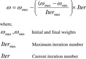
Two separately generated uniformly distributed random numbers in the range [0, 1]

The following weighting function is usually utilized:

Iter



_















max min max max

(



(14)

where,

min max

,



Initial and final weights

max

Iter

Maximum iteration number

Iter

Current iteration number

Suitable selection of inertia weight in above equation provides a balance between global and local explorations, thus requiring less number of iterations on an average to find a sufficient optimal solution. As originally developed, inertia weight often decreases linearly from about 0.9 to 0.4 during a run.

The algorithmic steps involved in particle swarm optimization technique are as follows:

1) Select the various parameters of PSO.

2) Initialize a population of particles with random positions and velocities in the problem space.

3) Evaluate the desired optimization fitness function for each particle.

4) For each individual particle, compare the particles fitness value with its Pbest. If the current value is better than the Pbest value, then set this value as the Pbest for agent i.

5) Identify the particle that has the best fitness value. The value of its fitness function is identified as Gbest.

6) Compute the new velocities and positions of the particles according to equation (12) & (13).

7) Repeat steps 3-6 until the stopping criterion of maximum generations is met.

4. RESULTS AND DISCUSSIONS

The applicability and validity of the proposed evolutionary algorithm for practical applications have been tested on various test cases consisting of 3-units and 6-units system [18, 19]. A reasonable B-loss coefficients matrix of power system network has been employed to calculate the transmission

losses. The software is developed in MATLAB and executed on Pentium IV PC (2.80 GHz) with 2.046 GB RAM.

Case 1: 3-units system

[image:4.595.320.540.170.316.2]

In this case, a simple power system consists of three-unit thermal power plant is used to demonstrate how the work of the proposed approach. Characteristics of thermal units are given in Table 1, the following coefficient matrix Bij losses.

Table 1 Generating unit capacity and coefficients

Unit

min

i

P

(MW)

max

i

P

(MW) ai

($/MW2₎

bi

($/MW) ci

($)

1 50 250 0.00525 8.663 328.13

2 5 150 0.00609 10.04 136.91

3 15 100 0.00592 9.76 59.16

  

 

  

  

000161 . 0 0002830 . 0 000184 . 0

000283 . 0 0001540 . 0 000175 . 0

000184 . 0 0000175 . 0 000136 . 0

ij B

[image:4.595.54.221.257.372.2]

Economic load dispatch (ELD) solution for three-unit system is solved using evolutionary algorithms such as DE, ABC, and PSO. Table 2 shows the optimal power output, total cost of generation, as well as active power loss for the power demands of 275 MW, 300 MW, 350 MW and 400 MW. It showed that the evolutionary algorithm has succeeded in finding a global optimal solution for this case.

Table 2 Comparison of three methods: best result for case 1

PDemand

(MW) Methods P1 (MW)

P2 (MW)

P3 (MW)

PLoss (MW)

Fcost ($/hr)

275 DE ABC PSO

189.95 189.95 185.82

70.44 70.44 73.42

23.40 23.40 24.57

8.80 8.80 8.80

3328.3 3328.3 3328.5

300 DE ABC PSO

202.47 202.47 202.59

80.98 80.98 81.40

27.08 27.08 26.50

10.54 10.54 10.49

3615.1 3615.1 3615.1

350 DE ABC PSO

228.08 228.08 227.26

102.62 102.61 102.91

33.81 33.81 34.38

14.50 14.50 14.54

4204.3 4204.3 4204.3

400 DE ABC PSO

250.00 249.84 248.45

126.64 130.56 129.74

42.72 38.48 40.94

19.36 18.87 19.14

4815.0 4815.2 4815.3

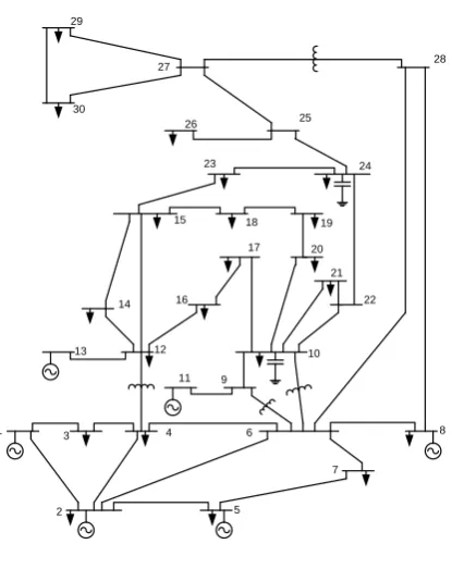
Case 2: 6-units system

To verify the effectiveness of the proposed evolutionary algorithm, a six-unit thermal power generating plant acquired from the standard IEEE 30 bus- test system (Figure 1) was tested. Characteristics of thermal units are given in Table 3, the following coefficient matrix Bij losses.

[image:4.595.315.550.422.556.2]

(5)

1

2 5

7

8 6

4 3

11 9

10 12

13

14 16 22

21 20

19 18

15

17

23 24

25 26

30 29

27 28

Figure 1: IEEE 30-bus 6-generator test system

Table 3 Generating unit capacity and coefficients

Unit

min i P

(MW)

max i P

(MW)

ai

($/MW2) bi

($/MW)

ci ($)

1 10 125 0.0033870 0.856440 16.817750 2 10 150 0.0023500 1.025760 10.029450 3 35 225 0.0006230 0.897700 23.333280 4 35 210 0.0007880 0.851234 27.634000 5 130 325 0.0004690 0.807285 36.856880 6 125 315 0.0003998 0.850454 30.147980

       

 

       

 



000085 . 0 000032 . 0 000025 . 0 000019 . 0 000020 0 000022 . 0

000032 . 0 000069 . 0 000030 . 0 000024 . 0 000015 0 000026 . 0

000025 . 0 000030 . 0 000071 . 0 000017 . 0 000016 0 000019 . 0

000019 . 0 000024 . 0 000017 . 0 000065 . 0 000013 0 000015 . 0

000020 . 0 000015 . 0 000016 . 0 000013 . 0 000060 0 000017 . 0

000022 . 0 000026 . 0 000019 . 0 000015 . 0 000017 0 000140 . 0

. . . . . .

[image:5.595.61.269.67.329.2]

Bij

Table 4 Comparison of three methods: best result for case 2 with PD = 700 MW

Unit Output DE ABC PSO

P1 (MW) 28.3056 27.3761 35.2774

P2 (MW) 10.0000 10.5000 40.3285

P3 (MW) 118.9572 118.7326 130.3539 P4 (MW) 118.6410 118.9831 125.1370 P5 (MW) 230.8075 230.6243 212.2078 P6 (MW) 212.7207 212.7142 174.5335 Total power

output (MW) 700.4319 718.9303 717.8380 Total generation

cost ($/hr) 820.2665 820.2667 823.9455 Power losses

(MW) 19.4319 18.9303 17.8380

CPU time (sec) 0.7773 2.0688 3.6866

P1 (MW) 32.5970 32.5652 38.0626

P2 (MW) 14.5060 14.4528 38.1482

(MW) 25.3327 25.3461 24.0292

CPU time (sec) 0.7658 2.0360 3.7776

P1 (MW) 36.8560 37.2907 52.9447

P2 (MW) 21.0658 24.2945 27.2979

(MW) 31.9858 31.8325 30.9183

CPU time (sec) 0.7610 2.0377 3.8754

5. CONCLUSION

In this paper a comparative study of different evolutionary techniques to solve the power system economic load dispatch problem is investigated. The proposed approach has been demonstrated by two different cases to have superior features, including high quality solution, stable convergence characteristic, and good computation efficiency. The simulation results obtained that the DE algorithm reaches convergence faster than ABC and PSO methods. However, the proposed three different evolutionary algorithms showed a good performance by reducing total operating costs and transmission losses.

6. REFERENCES

[1] B. H. Chowdhury and S. Rahman. 1990. “A review of recent advances in economic dispatch,” IEEE Transactions on Power Systems, vol. 5 (4), pp. 1248-1259

[2] A. J. Wood and B. F. Wollenberg. 1984. “Power Generation, Operation, and Control”, John Wiley and Sons, New York

[3] J. B. Park, K. S. Lee, J. R. Shin and K. Y. Lee. 2005. “A particle swarm optimization for economic dispatch with non smooth cost functions”, IEEE Trans. on Power Systems, vol. 20 (1), pp. 34-42

[image:5.595.54.263.611.751.2]

(6)

[5] K. Lenin and M. R. Mohan. 2006. “Ant colony search algorithm for optimal reactive power optimization”, Serbian Journal of electrical Engineering, vol. 3 (1), pp. 77-88

[6] H. T. Yang, P. C. Yang and C. L. Huang. 1996. “Evolutionary programming based economic dispatch for units with non-smooth fuel cost functions”, IEEE Transactions on Power Systems, vol. 11 (1), pp. 112-118 [7] W. M. Lin, F. S. Cheng and M. T. Tsay. 2002. “An

improved tabu search for economic dispatch with multiple minima”, IEEE Trans. on Power Systems, vol. 17 (1), pp.108-112

[8] Nasimul Nomana, Hitoshi Iba. 2008. “Differential evolution for economic load dispatch problems”, Electric Power Systems Research, vol. 78, pp. 1322-1331 [9] Pancholi, R. K., and Swarup, K. S. 2004. “Particle

swarm optimization for security constrained economic dispatch”, International Conference on Intelligent Sensing and Information Processing, Chennai, India, pp. 712

[10]H. Gozde, M. C. Taplamacioglu, and I. Kocaarslan. 2010. “Application of artificial bee colony algorithm in an automatic voltage regulator (AVR) system”, vol. 2 (4), pp. 88-92

[11]R. Storn, and K.V. Price. 1997. “Differential evolution a simple and efficient heuristic for global optimization over continuous spaces”, J. Global Optim. Vol. 11 (4) , pp. 341–359

[12]K. V. Price, R. M. Storn, and J. A. Lampinen. 2005. “ Differential evolution: a practical approach to global optimization”, Springer, Berlin, Heidelberg

[13]T. Takahama, and S. Sakai. 2006. “Constrained optimization by the epsilon constrained differential evolution with gradient-based mutation and feasible elites”, Proceedings of the 2006 IEEE Congress on Evolutionary Computation, pp. 308–315.

[14]D. Karaboga, and B. Basturk. 2008. “On the performance of artificial bee colony (ABC) algorithm”, Applied Soft Computing, vol. 8 (1), pp. 687- 697

[15]Dervis Karaboga, and Bahriye Akay. 2009. “A comparative study of artificial bee colony algorithm”, App. Mathematics and Computation, Elsevier, pp.108-132

[16]J. Kennedy, and R. C. Eberhart. 1995. “Particle swarm optimization”, Proceedings of IEEE International Conference on Neural Networks (ICNN’95), Perth, Australia, vol. 4, pp. 1942-1948

[17]Y. Shi and R. C. Eberhart. 2001. “Particle swarm optimization: development, applications, and resources, Proceedings of the 2001 Congress on Evolutionary Computation, vol. 1, pp. 81-86

[18]M. Vanitha, and K. Tanushkodi. 2011. “Solution to economic dispatch problem by differential evolution algorithm considering linear equality and inequality constrains”, International Journal of Research and Reviews in Electrical and Computer Engineering, vol. 1(1), pp. 21-26