Speciation in Digital Organisms
Thesis by
Stephanie S. Chow
In Partial Fulfillment of the Requirements
for the Degree of
Doctor of Philosophy
California Institute of Technology
Pasadena, California
2005
c
2005
Stephanie S. Chow
Acknowledgements
I would like to thank my advisor, Dr. Christoph Adami, for his advice and guidance on
all aspects of my graduate career in his lab. He helped make this thesis a reality. I would
also like to thank Dr. Claus Wilke for his close collaboration and patience with my many
questions, which taught me a lot on how to properly conduct research. My thesis committee
asked me some very interesting questions: Dr. Michael Cross, Dr. Steven Quartz and Dr.
Barbara Wold. My fellow graduate students in the lab, past and present, contributed many
useful suggestions: Alan Hampton, Allan Drummond, Evan Dorn, Jesse Bloom and Robert
Forster.
In less direct ways, my friends made this thesis possible. Without their friendship,
support, and advice on many aspects of my work and life, the stresses of graduate school
would have been impossible to deal with, and life would be a lot less fun.
Finally, I would like to thank my parents and my sister. Their love, support, and high
expectations, not to mention the examples that they set in their own careers made a Ph.D.
Abstract
Current estimates of the number of species on Earth range from four to forty million total
species. Why are there so many species? The answer must include both ecology and
evolution. Ecology looks at the interactions between coexisting species, while evolution
tracks them through time. Both are required to understand aspects of environments which
promote speciation, and which promote species persistence in time.
The explanation for this biodiversity is still not well understood. I argue that resource
limitations are a major factor in the evolutionary origin of complex ecosystems with
inter-acting and persistent species. Through experiments with digital organisms in environment
with multiple limited resources, I show that thes conditions alone can be sufficient to
in-duce differentiation in a population. Moreover, the observed pattern of species number
distributions match patterns observed in nature. I develop a simple metric for phenotypic
distance for digital organisms, which permits quantitative analysis of similarities within,
and differences between species. This enables a clear species concept for digital
organ-isms that may also be applied to biological organorgan-isms, thus helping to clarify the biological
species concept. Finally, I will use this measurement methodology to predict species and
Contents
Acknowledgements iii
Abstract iv
1 Introduction 1
1.1 Speciation . . . 2
1.2 Single niches and competitive exclusion . . . 5
1.3 Multiple niches and adaptive radiation . . . 7
1.4 Motivation . . . 10
2 Avida 12 2.1 Overview of Avida . . . 14
2.2 Organisms in Avida . . . 15
2.3 Virtual hardware . . . 15
2.4 Genomes and Instruction Sets . . . 17
2.5 Mutations . . . 19
2.7 Resources and the rate of reproduction . . . 20
2.8 Experimental setup . . . 23
3 Species in Avida 25 3.1 Species concepts . . . 25
3.2 The digital species concept . . . 26
3.3 Species determination . . . 28
3.3.1 Phylogenetic distance . . . 28
3.3.2 Clustering and calibration . . . 30
4 Adaptive radiation and emergence of species 34 4.1 A single niche in Avida . . . 34
4.2 Multiple niches in Avida . . . 35
4.3 Patterns of differentiation and speciation . . . 36
4.3.1 Low diversity populations . . . 37
4.3.2 High diversity populations . . . 38
4.3.3 Time course of speciation . . . 39
4.3.4 Methods of adaptation . . . 41
5 Diversity and productivity 44 5.1 Measures of diversity . . . 44
5.2 Productivity and species in Avida . . . 45
5.4 Frequency-dependent selection and stability . . . 51
5.4.1 Phenotypes of co-evolved species . . . 54
5.5 The founder effect . . . 56
5.6 Population size limitations . . . 58
5.7 Cutoff dependence of the clustering algorithm . . . 60
6 On the orthogonal nature of species 62 6.1 A representation of phenotype in Avida . . . 63
6.2 Species orthogonality . . . 65
6.3 Invasion of novel species into stable environments . . . 67
7 Conclusions and future research 73 7.1 Conclusions . . . 73
7.2 Future research . . . 75
7.2.1 Vector representation and speciation in biological organisms . . . . 75
7.2.2 Natural extinction . . . 76
8 Appendix 78 8.1 Alternate measures of distance between two genotypes . . . 78
8.2 The default instruction set . . . 79
List of Figures
1.1 The kangaroo, native only to Australia, eats grasses and the shoots and leaves
of plants [106]. . . 3
1.2 The deer, and its relatives such as gazelles and antelope, are native to most
continents, but not Australia. It eats grasses and the shoots and leaves of
plants [107]. . . 4
1.3 Changes in average cell size in a population of E. coli during 3000
gener-ations of experimental evolution. The solid line shows a best fit of a step
function model. From [30]. . . 6
1.4 Three basic types of Pseudomonas fluorescens morphs arising as a result
of adaptive radiation in an unshaken medium. The ’smooth morph’ (SM)
occupies the broth phase, ’wrinkly spreader’ (WS) occupies the air-broth
interface at the surface, and ’fuzzy spreader’ (FS) occupies the bottom of the
1.5 Diversity as a function of nutrient concentration in one replicate with
Pseu-domonas fluorescens. Black dots represent heterogeneous (undisturbed)
en-vironments, while white dots represent homogeneous (shaken) environments.
P-values for the quadratic effect are<0.0005 in the heterogeneous case, and
0.06 in the homogeneous case. Diversity is given as Simpson’s Index of
Diversity 1−λ. From [47]. . . 9
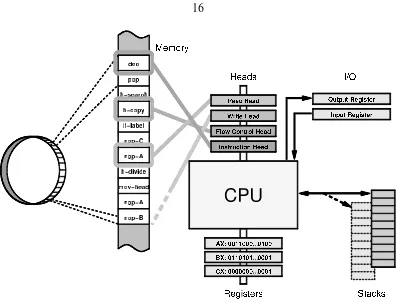
2.1 The basic hardware architecture of an Avida organism: CPU, registers, stacks,
IO buffers. From [72]. . . 16
3.1 A simple example of a phylogenetic tree, showing how to measure the
phy-logenetic distance between any two organisms or genotypes who share a
common ancestor. Each dot or node represents a genotype. Each edge
con-nects a parent genotype with a child genotype which is at least one mutation
away from its parent. In this example, A is the ancestor of all the genotypes
in the tree. The distance between any two nodes can be found by counting
the number of edges between them. The distance between B and its ancestor
3.2 Adjusted log cumulative proportion of replicates versus the second cluster
score in infinite (non-depletable) inflow runs. The values in the ordinate have
been transformed by adding one before taking the base 10 logarithm. The
solid line is the best linear fit through the origin. A cluster score threshold
of 151,467 classifies 75% of the infinite inflow replicates as having a single
species. . . 32
4.1 Fitness of E. coli in a glucose-limited environment. Fitness is measured
by calculating the reproductive rate of the population relative to that of the
founder, and displays punctuated increases as fitter mutants sweep through
the population. (data from R. Lenski, MSU) . . . 35
4.2 Fitness of digital organisms in Avida in a single niche environment. Fitness
is measured by the reproductive rate, and displays punctuated increases as
fitter mutants sweep through the population. . . 36
4.3 Phylogenetic depth versus time in an environment that does not promote
speciation. Each line traces an organism in the final population back to the
original unevolved ancestor. From [103]. . . 37
4.4 Phylogenetic depth versus time in an environment that does promote
specia-tion. Each line traces an organism in the final population back to the original
4.5 Resource use pattern as a function of time in a community of four species in
an experiment seeded with an unevolved ancestor. Black areas indicate that
a given resource is used at a particular point in time. Each subplot of the four
corresponds to the line of descent from a representative genotype (the most
numerous one) of one of the four species in the evolved population. Species
subplots are sorted in order of their time of branching from the main line of
descent, with the top one branching first, and so on. The experiment had the
standard duration of 400,000 updates, but only the first 200,000 are shown
since there are no subsequent changes to the figure. . . 40
4.6 Resource usage pattern as a function of time in a community of four species
in an experiment seeded with an evolved generalist who consumes all nine
resources. Black areas indicate that a given particular point in time. Each
subplot corresponds to the line of descent from a representative genotype
(the most numerous one) of one of the four species in the evolved population.
Species subplots are sorted in order of their time of branching from the main
line of descent, with the top one branching first, and so on. The full duration
5.1 Diversity in relation to productivity as a result of adaptive radiation in
Pseu-domonas fluorescens, by disturbance regime. More frequent disturbances
produce more homogeneous environments. Rows correspond to the
distur-bance regime, and columns correspond to different diversity measures. In
the first column, diversity is expressed as 1−λ (solid line) and λ1 (dashed
line); in the second column, as the number of distinct colony morphs; in the
third column, as the relative frequency of the smooth morphotypes (filled
sections) with respect to other types. From [48]. . . 46
5.2 Mean number of species as a function of inflow rate (A) and time (B). Error
bars indicate standard error over 25 replicates. All runs are seeded with an
unevolved ancestor unable to use any resources. From [6]. . . 47
5.3 Number of resources consumed by the population, by inflow rate and time.
At each time point, number of resources consumed by at least one member of
the population in a replicate is counted. For clarity, only every second inflow
rate, plus the infinite (non-depletable) case, is plotted. At a very low inflow
rate, few resources are exploited. At intermediate inflows, all or nearly all
nine are consumed, and at extremely high and infinite inflow rates, an
5.4 Mean time until first consumption of a resource, in replicates where the
re-source was used. A higher time value implies a more difficult gene to
ac-quire. Note: populations were sampled every 10000 updates, so transitory
genes may escape detection. If there is no data point, the gene was not found
in any replicate. . . 50
5.5 Relative fitness of a phenotype in a two-phenotype population as a function
of its proportion in the population, illustrating positive (A) and negative (B)
frequency-dependent selection. In A and B, a population consisting of 20%
phenotype 1 and 80% phenotype 2 has a relative fitness ratio of 1, indicating
that the two phenotypes are in equilibrium. In A, the equilibrium is unstable.
If phenotype 1 goes over 20% of the population, then it will be fitter than
phenotype 2 and increase its proportion in the population until it takes over.
Conversely, if phenotype 1 is below 20%, it will be less fit than phenotype 2
and go to extinction. In B, the equilibrium stable. If phenotype 1 is at
pro-portion greater than its equilibrium, it has a lower fitness than its competitor
phenotype 2, and will decrease in frequency. Conversely, if phenotype 1 is
at a lower proportion than equilibrium, it will be fitter than phenotype 2, and
5.6 Species invasion when rare in a replicate with six species. Each species in
the replicate is able to invade a population of the remaining five, where each
species is represented by its most numerous genotype. The effect of negative
frequency dependent selection is clear, as species adjust their numbers until
an equilibrium is reached. From [6]. . . 53
5.7 Matrix of resource use by the species depicted in figure 5.6. Each rectangle is
shaded according to the number of times the particular resource is consumed
in the life cycle of an average member of the species. Although there is some
overlap in resource use, each species dominates in at least one. . . 55
5.8 Mean number of species as a function of inflow rate where runs are seeded
with evolved generalist organisms. Error bars indicate standard error over 25
replicates. All runs are seeded with a clonal population based on one of five
generalists who use all nine resources. . . 57
5.9 Matrix of resource use by in a replicate with six species with a generalist
founder. Each rectangle is shaded according to the number of times it is
used in the life cycle of an average member of the species. Although there is
some overlap in resource use, each species dominates in at least one. . . 58
5.10 Mean number of species as a function of inflow rate per organism (A) and
population (B). Error bars indicate standard error over 25 replicates. All runs
5.11 Mean number of species as a function of the cutoff percentage of the species
clustering algorithm. Error bars indicate standard error over 25 replicates.
The cutoff proportion is the estimated probability that an infinite (non-depletable)
inflow replicate is determined to have one species rather than two. The
es-timate is derived from a linear fit through the origin of the log-transformed
cluster scores. . . 61
6.1 Computation profile of an Avida organism. In vector form, the profile is
(96, 0, 0, 0, 96, 0, 95, 0, 0). The values are taken from the most numerous
genotype in the replicate of figures 5.6 and 5.7. . . 63
6.2 The angleθbetween two vectors a and b. . . 64
6.3 Pairwise between-species and within-species task profile angles by inflow.
Between-species values are calculated over all pairwise angles between
co-evolved species, where a species is represented by its most numerous
geno-type at 400000 updates. The within-species values are calculated over all the
pairwise angles within a species. Error bars indicate standard error in the 17,
111, 90, 97, and 35 pairs of species at inflows of 1, 10, 100, 1000, and 10000
respectively. Inflows rates of 0.1 and 100000 are omitted because there were
6.4 Species populations as an invader is introduced into a stable 5-species
ecosys-tem. The invader is represented by a black line, while the various ecosystem
species are represented by coloured lines. The invader replaces one of the
ecosystem species (cyan). . . 69
6.5 Proportion of extinctions following the invasion of a novel species that
in-volve or do not inin-volve the closest competitor species to an invader. The
closest competitor of an invader is the species whose phenotype makes the
Chapter 1
Introduction
Life is found everywhere on Earth, and its variety is impressive. Microbes have been found
in Lake Vostok, which lies beneath the Antarctic ice sheet and is subject to high pressure
(350 atmospheres), low temperatures (-3o) and permanent darkness [88]. At another
ex-treme, evidence of microbes has also been found in oceanic volcanic glass [34]. The total
number of species may lie somewhere between 3 and 30 million [62], while some estimate
that there may be more than a billion species of bacteria alone [27].
What is the source of this range and variety? Charles Darwin addressed these issues
in his famous 1859 book “On the Origin of Species by Means of Natural Selection” [13].
Nearly one hundred and fifty years later, an understanding of the origin of species, or
speciation, remains incomplete. Although there is an outline of a theory of speciation,
the details of the causes and processes by which diversity and complexity arise and are
1.1
Speciation
The most important cause of speciation is geography. If a population of organisms from a
single species experiences restricted movement due to geographic barriers such as dry land
(for aquatic species), or mountains, the free flow of genetic materials within the species
is impeded. For the subpopulations divided by the barrier, isolation leads to independent
processes of natural selection and drift. Under different ecological conditions, the
subpop-ulations can diverge significantly [84]. After sufficient time, they may become different
enough to be called two species. Sexually reproducing organisms may diverge enough to
lose the ability to recombine genetic material, after which the two subpopulations will have
split permanently [63]. This effect is called allopatric speciation.
Australia’s unique flora and fauna are good examples of allopatry. Approximately 45
million years ago, Australia became a separate continent, isolating its species and allowing
many of them to evolve independently of those on other continents. The kangaroo is a
grazer, eating grasses and the shoots and leaves of plants. Other animals with similar dietary
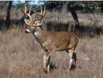
habits, but native to other continents, are the deer and its relatives such as gazelles and
antelope. In some ways, kangaroos and deer occupy the same niche on different continents,
an ecological term which can be defined as “a way of making a living”.
Less easy to explain is speciation in the absence of a geographic barrier, or sympatric
speciation. The finches of the Galapagos Islands, located 600 miles west of Ecuador, have
had a few million years to evolve. Thirteen species of finches that Darwin observed there
Figure 1.1: The kangaroo, native only to Australia, eats grasses and the shoots and leaves of plants [106].
or a few founders is called adaptive radiation. As the birds evolve, they fill different niches.
Some species eat seeds, others eat insects, and one drills for insects like a woodpecker.
Some live on the ground, some live in trees. Allopatric speciation has occurred, since
interbreeding is limited by the distance between the islands, but distinct species are also
found on the same island.
Much recent work in speciation has focused on models of sympatric speciation in
sex-ual organisms. Proposed explanations include assortative mating [86, 96], often due to
Figure 1.2: The deer, and its relatives such as gazelles and antelope, are native to most continents, but not Australia. It eats grasses and the shoots and leaves of plants [107].
selection [50], and offspring dispersal distance [49]. Ecological constraints have also been
cited as a cause of speciation in biological organisms [42, 84].
As can be seen from the diversity of finches in the Galapagos, ecological constraints
are a major source of evolutionary pressure. As the finches of the Galapagos increased
in numbers, they experienced increased competition for food. The population diversified,
adapting to different resources, as the challenge of finding nourishment provided an
in-centive to speciate in sympatry. Nonetheless, studies of evolution and ecology tend to be
separate, thus leaving the emergence of populations of differentiated, interacting organisms
This thesis will address the effect of environment on the emergence and maintenance of
diversity in asexual populations, as well as the limitations imposed on diversity by
ecologi-cal constraints. Sex and other forms of genetic recombination complicate the study of
evo-lution. In bacteria, for instance, the extent of recombination in bacteria varies widely [33],
and its effect is not necessarily beneficial [31, 51].
1.2
Single niches and competitive exclusion
The simplest type of environment is a homogeneous one with a single source of food. In this
environment, the genotype, or specific genetic makeup, that produces the best phenotype,
or set of physical traits, to consume the food and to power its reproduction is expected to
dominate the population, and to drive all other genotypes to extinction. When the frequency
of a gene has reached 100% of the population, this is called fixation. Only a single genotype
will be the best competitor for the single source of food, and its genes will tend to go to
fixation. The given set of conditions of the environment provides only one niche, which in
turn supports only one species. More niches support more species. There is “one niche,
one species”, a common way of phrasing the fundamental principle of ecology known as
the competitive exclusion principle.
The competitive exclusion principle states that in competition between species which
seek the same ecological niche, one species will outcompete the others. With a single
limiting resource, there may be more than one species co-existing, but one will be on its
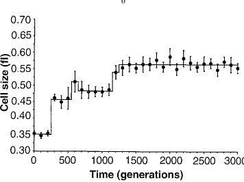
Figure 1.3: Changes in average cell size in a population of E. coli during 3000 generations of experimental evolution. The solid line shows a best fit of a step function model. From [30].
In a single niche environment, evolution occurs, but with a distinctive pattern. As
mutations occur, they may be either beneficial or deleterious. Although difficult to quantify,
studies of mutation rates in Caenorhabditis elegans [14] and Drosophila melanogaster [87]
indicate that mutations reduce fitness on average, so natural selection will tend to limit the
number of mutants. Rarely, there will be a beneficial mutation. Barring bad luck, this fitter
mutant will outcompete and out-reproduce its comrades; that is, the mutation will go to
fixation. Phenotypic changes often show a stepwise pattern, as seen in figure 1.3. These
periods of stasis alternating with brief periods of rapid change are an example of punctuated
equilibria [41]. The rate of beneficial mutations must be low to see this pattern [30]. At
clonal interference, as beneficial mutations compete with each other [39, 73].
1.3
Multiple niches and adaptive radiation
Recall that in allopatric speciation, geographic separation can induce differentiation.
An-other way that geography can promote differentiation in a population is through parapatric
speciation. An environmental gradient or change can result in adaptation to local
condi-tions in the absence of a explicit barrier to gene flow. In both cases, heterogeneity provides
niches and opportunities for mutants.
Adaptive radiation is the development of a variety of phenotypes from a single
ances-tral form. As the founders reproduce and mutate, the resulting population may rapidly fill
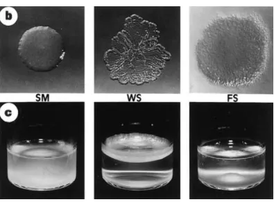
many ecological niches [85]. Figure 1.4 shows three morphologically distinct types, or
morphotypes, arising from adaptive radiation in the bacterium Pseudomonas fluorescens
propagated in a heterogeneous environment. Cultures of Pseudomonas fluorescens can
rapidly diversify their genotypes and phenotypes as they specialize into and adapt to
differ-ent environmdiffer-ents in the unstirred vessel containing the growth medium: the surface, liquid
phase and the bottom wall [78].
Another determinant of diversity or species richness in an ecosystem is productivity.
One definition of productivity is the rate of production of biomass in an ecosystem; the
mostly widely used is probably “the rate at which energy flows through an ecosystem” [81].
Species richness tends to increase with increasing ecosystem productivity, but is sometimes
Figure 1.4: Three basic types of Pseudomonas fluorescens morphs arising as a result of adaptive radiation in an unshaken medium. The ’smooth morph’ (SM) occupies the broth phase, ’wrinkly spreader’ (WS) occupies the air-broth interface at the surface, and ’fuzzy spreader’ (FS) occupies the bottom of the culture vessel. From [78].
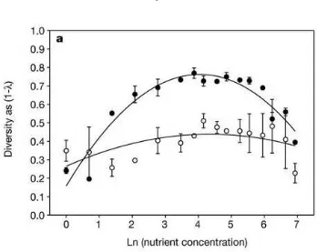
Two types of proposed diversity-productivity relationships are monotonically
increas-ing curves and unimodal (“hump-shaped”) curves, where diversity eventually decreases.
Data and theory mostly support unimodal curves [2,81,92] in heterogeneous environments,
although there is also support for monotonically increasing curves as well [1].
When cultures of Pseudomonas fluorescens are grown in heterogeneous environments
in a range of productivity levels, they show a clear unimodal diversity-productivity curve
[47], but show much less diversification in a homogeneous medium [47] [78], as seen in
Figure 1.5: Diversity as a function of nutrient concentration in one replicate with
Pseu-domonas fluorescens. Black dots represent heterogeneous (undisturbed) environments,
while white dots represent homogeneous (shaken) environments. P-values for the quadratic effect are<0.0005 in the heterogeneous case, and 0.06 in the homogeneous case. Diversity is given as Simpson’s Index of Diversity 1−λ. From [47].
Heterogeneity in the environment provides an opportunity for the emergence of stable
polymorphisms, and perhaps eventual speciation through allopatric or parapatric means.
Another way populations increase diversity is through resource partitioning, where
sub-populations minimize competition by focusing on different resources [61, 77], although
spatial structure can be a factor in the extent of differentiation. Escherichia coli grown in
a homogeneous medium with a single limiting sugar may undergo adaptive radiation via
cross-feeding, in which metabolites produced by certain phenotypes are consumed by other
1.4
Motivation
That environmental heterogeneity or multiple resources may induce differentiation and
adaptive radiation within a population has been established in experiments with
Pseu-domonas fluorescens and Escherichia coli. The question remains as to the necessity of
the first, and the limits of the second. The principles underlying the emergence and
main-tenance of a diverse population of organisms, as well as factors limiting its diversity, in a
resource-limited homogeneous environment are not yet well-understood.
The goal of my thesis research is to investigate speciation in well-stirred environments
with multiple limited resources through experiments with digital organisms. First, I will
address the issue of speciation, establishing a definition of species in digital organisms,
and examining the conditions for and dynamics of adaptive radiation and sympatric
spe-ciation [6, 103]. I will also look at the dynamics of adaptation of individual species in
the population [103]. Second, I will show that species richness peaks at intermediate
pro-ductivity [6], a pattern which matches some experimental observations such as the ones in
figure 1.5. Furthermore, this pattern is observed without relying on environmental
hetero-geneity as in many models and experiments. Factors which support long-term coexistence
and stability in evolved ecosystems are also elucidated and tested. Third, I will show that
the coevolved species show distinctive phenotypic characteristics relative to each other. I
will continue on to develop a measure of phenotypic difference, and use it to show that
this measure verifies a fundamental ecological principle with respect to the definition of a
Chapter 2
Avida
While the ecology and evolution literature may cover the full range of life on earth,
ex-perimentalists often limit themselves to a much smaller selection. Bacteria are a common
experimental organism in evolution, as are viruses and yeast [32], since they satisfy to
var-ious degrees the following list of desirable properties for organisms that can be used for
experimental evolution research:
• Organisms are abundant and easy to breed.
• Organisms have a short generation time.
• The experimental environment that organisms live in is simple and controllable.
• It is easy to make measurements of genotypic and phenotypic characteristics.
• It is easy to store historical lineages.
Other organisms less commonly used for experimental evolution include multicellular
Although bacteria are easily propagated, have fairly short generation times, and are
easy to grow, evolution experiments are still very time-consuming. One generation of E.
coli takes approximately 20 minutes under optimal conditions. In practice, experimental
conditions rarely allow reproduction to proceed at the maximum possible rate. Experiments
with E. coli may run for 10000 generations [58, 76], and long-term studies have gone for
20000 generations or more [83]. Moreover, the observation of cross-feeding [43, 82, 83,
95, 97], where some bacteria consume the waste products of others, shows that aspects
of environment can be difficult to control precisely. Finally, sufficient measurements of
fitness, genomics and other data for high statistical accuracy may be impractical. One
solution to these problems is to use digital organisms, which share many properties of
biological organisms [102], but exceed them in others.
Digital organisms are self-replicating computer programs that have the three necessary
and sufficient ingredients for Darwinian evolution. These are mutation (variation),
replica-tion (inheritance) and differential fitness (selecreplica-tion). They live in, and adapt to, an
environ-ment controlled by the experienviron-menter. The complexity of the organism conferred by their
computational genomic basis leads to complexity in their behaviours, complexity in their
interactions, and evolutionary population dynamics among others. Recent studies with
dig-ital organisms have addressed issues of genome complexity and genetic interactions [56],
robustness to mutations [104] and the evolution of complex features [57].
Many other prior computational approaches to evolution have been simulations rather
2.1
Overview of Avida
The software platform for my experiments in computational evolutionary biology is called
Avida. It is free and open-source (downloadable at www.sourceforge.net). All
experi-ments were performed with version 1.99 of the Avida platform, compiled for linux with
gcc-2.95.
Avida is a computer software and genetic system in which a population of asexual
digital organisms evolves by natural selection. An organism is defined by its genome, a
self-reproducing string whose elements are commands from a Turing-complete instruction
set. Each genome executes on a virtual central processing unit (CPU). Mutations in an
or-ganism’s genome correspond to changes in its instruction string. These can be deleterious,
resulting at worst in an inability to reproduce, but may also be neutral or beneficial, for
instance increasing replication efficiency or adding functionality. Simple Darwinian
selec-tion will then act upon these new organisms as they compete with the rest of the populaselec-tion.
By correctly performing simple binary operations on up to three arbitrary 32 bit numbers,
an organism increases its “merit”, which increases the speed of its virtual CPU relative to
other organisms. This, in turn, speeds up its reproduction.
The software has three main modules. The first is the Avida core, which maintains a
population of digital organisms (genome or code, and virtual hardware), an environment
with reaction rules (artificial chemistry) and resources, a scheduler to allocate CPU cycles
to the organisms, and data collection objects. The second is the graphical user interface
analysis and statistics tools to collect data and perform analyses of organism properties,
lines of descent and many other features.
2.2
Organisms in Avida
Each organism in Avida is a self-contained automaton that can construct new automata.
The organism, following the instructions in its genome, uses its virtual hardware to interact
with the Avida environment as well as to attempt to make a perfect copy of its genome. The
new genome is then passed to the Avida world, which gives the (possibly imperfect) copy
its own virtual hardware, and places it somewhere in the population. If the environment
has a grid structure, then the new offspring may be put in a location adjacent to the parent.
If the environment is modelled on a chemostat and therefore has no spatial structure, the
offspring may be be put in any random location. In either case, the Avida world has a fixed
population size, so placing an offspring in a location means first killing and removing the
previous occupant.
2.3
Virtual hardware
The basic structure of an Avida machine or organism is shown in figure 2.1. At the core
is the CPU, which executes the instructions in the genome, and modifies the states of its
components accordingly. There are three registers to store and manipulate data in the form
Figure 2.1: The basic hardware architecture of an Avida organism: CPU, registers, stacks, IO buffers. From [72].
At the initialization of an organism, the genome is loaded into memory. Execution starts
with the first instruction and proceeds sequentially, unless an instruction (such as a jump)
explicitly commands otherwise. When the last instruction is reached, the program loops
back to the beginning. In effect, the genome is circular, just as in most types of bacteria.
The CPU structure supports four heads, which are essentially pointers to locations in
memory: the instruction head, which points to the location of the instruction being
exe-cuted; the read head and write head, which together allow the organism to read an
instruc-tion at one locainstruc-tion and write it to another; and the flow-control head used for jumps and
Finally, there is an input buffer and an output buffer, which allow the organism to
inter-act with the environment. The machine can read in one or more inputs, perform
computa-tions, and write the results to the output buffer.
2.4
Genomes and Instruction Sets
As in biological organisms, it is the order and combination of the basic units of genetic
information that define the genome. The elements of the assembly-like language are part of
the full range of instructions that can be executed by the Avida CPU. Certain subsets of the
instructions, called “instruction sets”, form logical units, each of which can be considered
a programming language. A genome is a sequence of instructions from the instruction set,
in the way DNA is a sequence of bases from the set of four nucleotides.
The instruction set used for the experiments in this thesis is the default instruction set,
consisting of the following 26 instructions:
nand IO h-alloc h-divide h-copy h-search mov-head jmp-head get-head if-label set-flow
The first three instructions are thenop(“no-operation”) instructions, which do nothing
on their own, as their name suggests. They are used for template matching, like labels. For
example, positions in the genome can be tagged, allowing jumps and function calls to go
to the right place even if the genome is subject to change, especially insertion and deletion
mutations that shift instruction positions. Nops have circular complementarity: the
comple-ment ofnop-Aisnop-B, the complement ofnop-Bisnop-C, and the complement ofnop-C
isnop-A. For example,h-search nop-A nop-B mov-head ... nop-B nop-Cputs the
flow-control head after the complement tonop-A nopB, that is, after nop-B nop-C. Then
mov-headmoves the instruction head to the position of the flow-control head, and
execu-tion of the genome continues from the new posiexecu-tion. Nops can also be used as arguments
to the preceeding instruction. For example,inc nop-Aincrements theAXregister.
To replicate, h-allocallocates memory at the end of the genome for a copy,h-copy
works with other structures in the hardware to create the copy, and h-divide splits the
doubled genome in two, passing the copy to Avida which uses it to create a new organism
in the world.
example of a genome, which can copy itself and nothing more.
h-alloc # Allocate space for child
h-search # Locate the end of the organism
nop-C #
nop-A #
mov-head # Place write-head at beginning of offspring.
nop-C # Insert as required to achieve desired genome length h-search # Mark the beginning of the copy loop
h-copy # Do the copy
if-label # If we’re done copying...
nop-C #
nop-A #
h-divide # ...divide!
mov-head # Otherwise, go back to the beginning of the copy loop. nop-A # End label.
nop-B #
In summary, a self-replicating genome typically allocates space for the offspring, puts
the write head at the beginning of the allocated space, iteratively copies each instruction to
the child segment of the expanded genome, and then divides. The seed organism used in
many of the experiments in this thesis has an almost identical genome, but with many more
nop-C’s as placeholders to extend the genome length for reasons detailed later.
2.5
Mutations
The variability in the population that is required for selection is provided by mutations in
the genome. The main type is the copy mutation. With a probability set by the
experi-menter, the instructionh-copydoes not copy the instruction pointed to by the read head,
but instead writes a random instruction to the location pointed to by the write head. Other
inser-tion and deleinser-tion mutainser-tions, which may insert or delete a random instrucinser-tion in the child
organism; and cosmic-ray or point mutations, in which random changes in the genome
occur during its execution at a set rate. A final type is the implicit mutation, caused not
by explicitly set mutation parameters, but by an incorrect copy algorithm. Offspring with
these mutations can be automatically discarded by setting theFAIL IMPLICIToption in the
genesis configuration file.
2.6
The Avida world
The Avida world has a fixed number N of cells or positions, each of which can hold at most
one organism. The maximum population size is therefore also N. There are two possible
topologies: a 2D grid with Moore neighbourhoods (each cell has eight neighbours), and a
fully connected or well-stirred topology, where every cell is a neighbour to every other cell,
and there is in effect no spatial structure. When an organism reproduces, depending on the
parameter set by the experimenter, the offspring is placed in a random cell in the
neigh-bourhood, or in the oldest cell (with a preference for empty cells) in the neighbourhood.
The experiments in this thesis use the well-stirred structure with random replacement.
2.7
Resources and the rate of reproduction
All organisms have a virtual CPU, and each CPU can run at a different speed. In the
executed per unit time). To simulate CPUs running in parallel, Avida provides a
sched-uler which executes one instruction on one machine, then one on another, and so on. A
unit of time in Avida is an update, a period in which the average organism has executed k
instructions (k=30 by default).
If speeds differ between organisms, then the scheduler allocates CPU cycles
propor-tional to the organism’s merit, a unitless value which has meaning only when compared
with the merits of other organisms. This allocation can be either perfectly integrated, or
probabilistic. The perfectly integrated is the default, and the one used for experiments in
this thesis.
All organisms start with an initial merit depending on their sequence length, since the
length affects the time required to reproduce. This gives them an initial CPU speed. An
Avida environment can contain resources that an organism can consume to change their
merit. To absorb a resource, the organism must carry out the corresponding computation,
or task as explained below.
The environment consists of a set of resources and a corresponding set of reactions
re-quired to interact with them. A reaction is defined by a computation that must be performed,
a resource that is consumed as a result, the effect on merit (which may be proportional to the
amount available in the environment), and a possible by-product. A resource has an initial
level, an inflow rate in units per update, and an outflow rate as a fraction of the amount in
the environment per update. If inflows are finite, then the resources are depletable, so that
that resource. “Infinite” inflows are possible by making resources non-depletable.
Reac-tions can have condiReac-tions to control when they will be successful and therefore when they
can change merit. These conditions could be a limit on the number of times a reaction can
be performed, or be a requirement that another reaction must have been triggered first.
For natural selection to occur in Avida, there must be variability in the rate of
repro-duction, and some limit on population size. In a given organism, this is determined by
a combination of CPU speed and gestation time, the number of instructions it needs to
execute to produce an offspring.
To summarize, there are three types of resources in Avida. First, there is the basal
re-source, which is available to all organisms and allows them to replicate even if they cannot
compute any logic functions. Second, there are computational resources which can be
as-sociated with the logic functions. There are plans to remove the basal resource in future
versions of Avida, so that organisms can survive only when they can utilize computational
resources, but currently, the basal resource is always available to every organism, and
can-not be depleted. Finally, there is space. The memory of the virtual computer in which the
Avida organisms live can hold only a finite number of organisms, which are replaced at
random when new organisms are born.
It is important to note that in Avida, rewards do not depend on how the computation is
performed. Avida presents the organism with inputs, and looks for a an output
2.8
Experimental setup
For the experiments in this thesis, the environment has nine resources corresponding to
nine simple one and two input logical functions: Not, Nand, And, OrNot, Or, AndNot,
Nor, Xor, and Equals. Resource levels start at zero, flow in at a constant rate, and flow out
at a rate of one percent. The following are other basic features of the experiments:
• Population size of 3000
• Fixed genome length of 100
• Experiment duration of 400000 updates
• Seeded with an unevolved ancestor, giving a clonal population
• Same inflow and outflow rates for all resources, which give the same reward per unit
consumed
• Inflow rates varied over six orders of magnitude, from 0.1 units per update to 100000
units per update
• Copy (point) mutations only, with a per site probability of 0.005 (100×0.005=0.5
mutations per generation)
• No recombination
A population size of 3000 individuals is enough to allow maximum diversification
genome length simplifies analysis, since genomes are easily compared to each other. The
length is maintained by having only point mutations during the copy loop and
disregard-ing offsprdisregard-ing with other lengths (which can happen if the copy loop is faulty and splits the
offspring off at the wrong time). A length of 100 and an experiment duration of 400000
up-dates is more than sufficient for organisms to acquire all nine rewarded tasks if conditions
are favourable. The range of inflow rates is guided by the range in productivity required to
generate the hump-shaped diversity pattern in Pseudomonas fluorescens [78] as seen earlier
in figure 1.5.
In biological organisms, mutation and sometimes recombination provide the variability
in populations upon which natural selection acts. A genomic mutation rate (number of
mu-tations per generation) 0.5 allows evolution to occur quickly without adding too much noise
to the system. By comparison, the approximate genomic mutation rate in RNA viruses is
1, and in DNA-based microbes, it is much lower [24]. Since biological genomes are
sig-nificantly larger than the digital ones in these experiments, the genomic mutation rates
correspond to much lower per site and per gene mutation rates. Although recombination
or gene transfer is a factor in rates of bacterial evolution [37, 70], its extent in natural
pop-ulations varies between bacterial species [33] and its overall impact is not clear [31]. For
these reasons, as well as ease of tracing lines of descent, there is no recombination in these
Chapter 3
Species in Avida
The species is a unit of evolution and of classification, and its definition is important to
the study of speciation. And yet, Mallet notes that “we still do not all accept a common
definition of what a species is” [60]. The number of species is a widely used measure of
biodiversity, and will be used to measure diversity in digital organisms as well.
3.1
Species concepts
According to Darwin, the “undiscovered and undiscoverable essence of the term species”
meant that “we shall have to treat species in the same manner as those naturalists treat
genera, who admit that genera are merely artificial combinations made for convenience”
[13].
Since that time, there have been many more concrete species concepts – Coyne [10] lists
some recent ones: biological [19,63], evolutionary [101], phylogenetic [12,17], recognition
[59], cohesion [91], ecological [98] and internodal [52].
probably the best known. Species are “groups of interbreeding populations in nature,
unable to exchange genes with other such groups living in the same area” [63].
Al-though there are already many difficulties with the concept with respect to sexual
repro-duction [23, 60, 89], it is even harder to apply to asexual reprorepro-duction due to its reference
to the concepts of recombination or gene transfer.
It is well-known that some bacteria which differ significantly both genotypically and
phenotypically are still able to exchange genetic material [26]. Lateral (or horizontal) gene
transfer is a common phenomenon in bacteria and is an important factor in their
evolu-tion [37, 54, 70] although its extent varies significantly [33] and its effect is not necessarily
beneficial [31, 51]. Similarly, viral recombination is also common [35, 100]. Furthermore,
the exchange of genetic material has been shown to extend to gene transfers between
king-doms – between prokaryotes, eukaryotes and archaea [105], clearly not members of the
same species. Recombination is not a good basis for a species definition in asexual
organ-isms.
3.2
The digital species concept
Although consensus is lacking on a definition of species even when restricted to bacteria, a
solution is to omit rates of recombination or lateral gene transfer in the genome, or at least
treat it differently. In bacteria, definitions of species may rely on phylogeny or descent in
gene trees [28], which trace the lineage of a particular segment of DNA rather than the
cells in the same ecological niche [8]; a third is to combine taxonomy (classification based
on physical characteristics) and phylogeny [68].
Organisms in nature have been observed to form tight clusters [11, 40] rather than a
continuum, although successive species sometimes coexist for a time [41]. In a single
niche, organisms form a single cluster, implied by the stepwise pattern seen earlier in figure
1.3. A species can be considered to be a collection of genotypes which share many common
genotypic and phenotypic features with each other, but differ considerably from members
of other species [60], a definition which has been used for bacterial species [7, 77].
I will base the concept of a digital species on phylogeny, an important tool in evolution
[74]. Organisms which are closely related, i.e., have recent common ancestors, are more
likely to be of the same species than more distantly related ones. Recall that there is no
recombination in my experiments, so relatedness is easy to measure. Underlying the use
of phylogenetic information is the hypothesis, supported by results reported in this thesis,
that closely related organisms also share common genotypic and phenotypic features. By
the phenotype of a digital organism, I am referring to the ecological niche, or pattern of
Time
B
C
[image:44.595.124.525.70.260.2]A
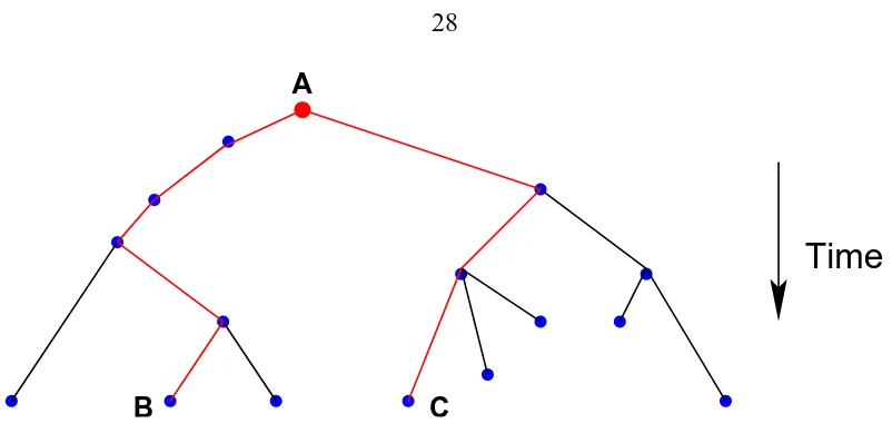
Figure 3.1: A simple example of a phylogenetic tree, showing how to measure the phylo-genetic distance between any two organisms or genotypes who share a common ancestor. Each dot or node represents a genotype. Each edge connects a parent genotype with a child genotype which is at least one mutation away from its parent. In this example, A is the ancestor of all the genotypes in the tree. The distance between any two nodes can be found by counting the number of edges between them. The distance between B and its ancestor A is 5, and the distance between B and C is 8.
3.3
Species determination
3.3.1
Phylogenetic distance
To measure relatedness of two genotypes, I use phylogenetic distance. Avida can output a
complete record of every genotype in the population as well as every genotype in the lines
of descent all the way back to the seeding population. Each record includes the genome,
useful data such as the current and past numbers of organisms with this genotype, as well
as an identifier of the parent genotype. With the lineage information, it is simple to recreate
a phylogenetic tree (or trees for non-clonal seed populations) which contains the entire
ancestry of every genotype in the current update. Each edge of the tree joins a parent
mutations (a second mutation which changes the genome back to the original), multiple
mutations, and the more common single point mutations. Hamming distance, the number
of point to point differences between two strings of symbols, between an ancestral genotype
and its descendants increases with time, so back mutations are rare. Intuitively, since a
mutation picks a replacement with equal probability from the instruction set, and the default
instruction set has 26 possible instructions, back mutations are unlikely. Multiple mutations
are also very rare, given reasonable mutation rates.
The phylogenetic distance between any two genotypes in a tree is obtained by counting
the number of edges in a path (no repeated nodes) connecting the two genotypes. A simple
example is illustrated in figure 3.1. Start at either one of the genotypes, count up (i.e.,
back in time) the edges between child and parent genotypes in the tree to the most recent
common ancestor (MRCA) of both. Then continue counting down (i.e., forward in time)
the tree from the MRCA to the second genotype. If the MRCA is not known, start at one
genotype and flag its entire line of descent back to a known common ancestor. Then start
at the other genotype and trace its ancestry until you hit a flagged genotype. The flagged
genotype is the MRCA. The phylogenetic depth of a genotype to an ancestral genotype is
the number of mutants or edges in the tree between the two. The phylogenetic distance
between two genotypes is therefore equivalent to the sum of the phylogenetic depths of the
two organisms relative to their MRCA.
Other measures of distance between two genotypes include Hamming distance and time
they were both found to be inadequate for different reasons. Details are in the appendix.
Intuitively, a smaller phylogenetic distance between two genotypes implies increased
relatedness and a correspondingly increased likelihood of being members of the same
species. Similarly, for any subpopulation or cluster of organisms, a score based on the
pairwise distances between genotypes in the cluster, such as a sum, will indicate the
relat-edness within the cluster.
3.3.2
Clustering and calibration
The partitioning of the population into species is achieved by a clustering algorithm
de-signed by Charles Ofria expressly for species determination in digital organisms in Avida.
I coded the algorithm in C++ and it is available online [5].
In the clustering algorithm, all genotypes are initially in a single cluster, and this cluster
is given a score based on phylogenetic distance. The score is compared to a cutoff, and
cluster is repeatedly divided until the score falls below the cutoff. The final number of
clusters or species is not known in advance. The detailed steps are as follows:
1. Put all genotypes into a single, initial cluster.
2. Find the genotype that minimizes the sum of the distances from it to all the other
genotypes in the cluster; this is the centroid of the cluster.
3. Sum the distances; this is the score for the cluster.
5. Otherwise, search through the remaining non-centroid genotypes and find a new
cen-troid – the genotype which minimizes the sum of distances of all genotypes to the
nearest centroid.
6. The score of the new cluster is the sum of the distances.
7. Compare the cutoff to the new score. If the cutoff is greater than the total, stop.
8. Repeat the previous three steps as needed.
Recall that a single niche environment usually contains only one species, although
suc-cessive species sometimes coexist for a time [41]. In Avida, a single niche environment can
be created by making resources undepletable. The sole limit to growth is population size,
and the evolved population will usually have a single, dominant species.
If the single niche population is considered to be a single cluster, the resulting score
will be low since all genotypes are closely related. I will use the distribution of single niche
scores to determine a cutoff for the clustering algorithm.
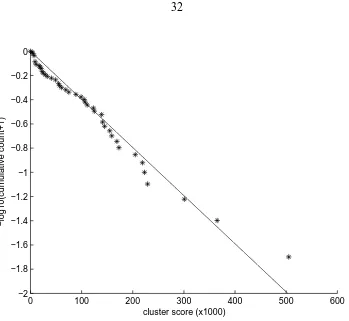
The setup for the calibration experiments matches the basic procedure in section 2.8
ex-cept that resources are undepletable. There are 50 replicates, each with the same virtual
en-vironment seeded with a population of 3000 clones of a simple, unevolved organism. When
I examined the resulting evolved populations, there were strong phenotypic and genotypic
similarities, suggesting that organisms were closely related. At 100,000, 200,000, 300,000,
and 400,000 updates, I calculated the score of a second cluster in the evolved replicate
0 100 200 300 400 500 600 −2
−1.8 −1.6 −1.4 −1.2 −1 −0.8 −0.6 −0.4 −0.2 0
cluster score (x1000)
[image:48.595.147.496.73.394.2]−log10(cumulative count+1)
Figure 3.2: Adjusted log cumulative proportion of replicates versus the second cluster score in infinite (non-depletable) inflow runs. The values in the ordinate have been transformed by adding one before taking the base 10 logarithm. The solid line is the best linear fit through the origin. A cluster score threshold of 151,467 classifies 75% of the infinite inflow replicates as having a single species.
since the population has not had much time to differentiate from its clonal beginning. At
updates 200,000, 300,00 and 400,000, the distributions of scores are quite similar. All of
the score distributions are well described by an exponential. I transformed the scores from
update 400,000 with log(1+cumulative counttotal count ), and calculated the linear best fit through the
origin in figure 3.2.
With the fitted function, I calculated cutoff scores at a variety of probabilities, where
pair. A probability of 75% of classifying the single niche population as one species works
well for sorting well-differentiated populations generated at intermediate inflow rates into
Chapter 4
Adaptive radiation and emergence of
species
The simplest ecosystem has a single niche. As discussed earlier in section 1.2, evolution
takes place via successive sweeps of increasingly fit genotypes. A plot of fitness in E. coli
in figure 4.1 shows a punctuated pattern, similar to the plot of cell size in figure 1.3.
4.1
A single niche in Avida
When digital organisms face a single niche environment, as in the threshold calibration
experiments detailed in section 3.3.2, their fitnesses in figure 4.2 are indistinguishable from
those of figure 4.1. Since resources are unlimited, the environment has no effect on growth
rates and thus the speed of reproduction is the only determinant of fitness. As fitter digital
organisms emerge through random mutation, selection causes the familiar pattern of long
Figure 4.1: Fitness of E. coli in a glucose-limited environment. Fitness is measured by cal-culating the reproductive rate of the population relative to that of the founder, and displays punctuated increases as fitter mutants sweep through the population. (data from R. Lenski, MSU)
4.2
Multiple niches in Avida
Adaptive radiation of a clonal population of bacteria can occur as a result of different
conditions, including seasonal environments, resource partitioning and spatial
heterogene-ity [78, 94]. The resulting evolved outcomes can be sensitive to small changes in
environ-mental conditions [58, 93, 94]. Bacteria propagated under identical environments
some-times achieve similar fitnesses [93], but other experiments have found that replicate
pop-ulations can diverge significantly from one another in morphology and mean fitness [58],
suggesting that random events play an important role in evolution.
When a well-stirred digital environment has limited supplies of multiple resources,
0 100000 200000 300000 400000 0
2 4 6 8 10
time [updates]
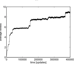
[image:52.595.168.481.83.352.2]average fitness
Figure 4.2: Fitness of digital organisms in Avida in a single niche environment. Fitness is measured by the reproductive rate, and displays punctuated increases as fitter mutants sweep through the population.
heterogeneity. The multiple resources provide an opportunity for organisms to minimize
competition by differentiating from each other, specializing into different niches.
Nonethe-less, a given environment may produce a wide range in the number of species. As seen
in bacteria [58], replicate populations propagated under identical conditions can diverge
significantly from one another.
4.3
Patterns of differentiation and speciation
When a lineage evolves, speciation can occur in one of two ways: the lineage may change
lin-0
100000
200000
300000
400000
0
500
1000
1500
Time [updates]
[image:53.595.125.517.80.403.2]Phylogenetic depth
Figure 4.3: Phylogenetic depth versus time in an environment that does not promote spe-ciation. Each line traces an organism in the final population back to the original unevolved ancestor. From [103].
eage may branch into new forms, called cladogenesis. The earlier figures 1.3 and 4.1 with
their punctuated pattern, suggest anagenesis, while the morphotypes of Pseudomonas
fluo-rescens in figure 1.4 suggest cladogenesis.
Multiple niche environments can exhibit both forms of speciation.
4.3.1
Low diversity populations
Figure 4.3 shows a typical phylogenetic depth pattern for a community of digital
descent quickly coalesce. The most recent common ancestor (MRCA) of the community
lived at around update 350,000, approximately 50,000 updates before the end of the
exper-iment. From the MRCA, a single line of descent leads back to the founding ancestor. The
small phylogenetic distance from an organism in the final population to the MRCA reflects
the strong genotypic and phenotypic similarities within the final population. Although in
this example the depletable resources were very abundant, this type of ecosystem evolved
at least once out of 50 replicates at every inflow rate.
4.3.2
High diversity populations
By contrast, figure 4.4 shows a typical phylogenetic depth pattern for a community of
digital organisms that has speciated. As before, each line traces an organism in the final
community backwards in time. This time, the lines of descent do not quickly coalesce.
There are four deep, clear branches that separate early, at around update 100,000. Near the
end of the experiment, at around updates 300,000 to 350,000, these four branches fan out
in the same way as the single branch in figure 4.4. The interpretation of this observation
is simple: In a community that has speciated, all organisms within a single species share a
fairly recent common ancestor, but the most recent common ancestor of all species lies in
0
100000
200000
300000
400000
0
100
200
300
400
500
600
700
800
Time [updates]
[image:55.595.131.507.84.407.2]Phylogenetic depth
Figure 4.4: Phylogenetic depth versus time in an environment that does promote speciation. Each line traces an organism in the final population back to the original unevolved ancestor. From [103].
4.3.3
Time course of speciation
In this section, I investigate the ways in which a community evolves. The alterations may
involve changes to the resources used, as well as phenotypic changes at branching points
of the lineage and at other times.
Figure 4.5 shows resources used as a function of time in a replicate resulting in four
species seeded with the basic unevolved ancestor. Species are numbered in order of
branch-ing. At the beginning of the experiment, rapid evolutionary change occurs, as organisms
of species 1 branches off from the rest of the population, and after branching, the lineage
changes its phenotype and then settles on resources 2 and 3. At update 80,000, the ancestor
of species 2, 3 and 4 has chosen other resources than species 1, consuming resources 1, 4
and 7. At update 110,000, species 3 and 4 branch off nearly simultaneously. By update
130,000, each species has settled on a different subset of resources. Some resources are
shared by more than one species, but no two species use the exact same set. There are no
changes to the four sets of resources used by the four species after update 130,000.
4.3.4
Methods of adaptation
The replicate in figure 4.5 above was seeded with a basic, unevolved genotype, so perhaps
it is not surprising that rapid changes in phenotype occurred at the beginning of the
experi-ment. Do rapid changes occur when a well-evolved seed genotype is used instead? Figure
4.6 shows resources used as a function of time in another replicate resulting in four species,
this one seeded with a generalist who uses all nine resources 1. The same basic
environ-ment with the same basic resource inflows was used. Note that figure 4.6 shows 400,000
rather than the 200,000 updates in figure 4.5, since the resource usage continued to change.
To contrast with the unevolved ancestor, the generalist seed was the most numerous (and
therefore successful) genotype in a population which had evolved for 400,000 updates.
In the beginning, rapid evolutionary change occurs, but not as rapidly as observed with
the unevolved ancestor. On the other hand, evolutionary change in resource usage continues
1Generalists are difficult to evolve unless the environment is specifically structured to reward the use of
for much longer. The first species emerges at approximately update 30,000, the second at
update 100,000, and the third and fourth split at update 160,000. The first two species to
emerge show few changes in resource usage after speciation, while the last two continue to
adapt. By the end of the experiment, perhaps thanks to the longer period of adaptation, all
four species have settled on non-overlapping resources: species 1 on resources 1, 2, 4 and
5; species 2 on 7; species 3 on 6, and species 4 on 8.
One method of adaptation is through gain of function, easily seen in the early updates
of figure 4.5. The various descendants of a genotype using no resources have acquired the
ability to use each one of the resources at some point in time.
Another less obvious method of adaptation is through loss of function, also observed
in bacteria [65, 71]. Loss of function can be seen in the early updates of figure 4.6, as
the descendants of the generalist adapt to new environment by differentiating, this time by
specializing on different resources to minimize competition.
The third important method of adaptation can be seen in both figures, more easily in the
middle to later updates, namely the gain by a lineage of one resource often coincides with
the loss of another, easily seen at update 90000 in species 2, 3 and 4 of figure 4.5, as well
as in the switching of species 3 in 4.6 between resources 3 and 6 between updates 250,000
to 310,000. In the genomes of this section of the lineage, the code to use resource 3 is is
derived from the code to use resource 6, and vice versa. This adaptation of existing genetic
Chapter 5
Diversity and productivity
Since digital environments can produce differentiated populations under conditions of
mul-tiple, but limited, resources, as can the biological ones described in section 1.3, will the
resulting pattern of diversity in response to resource supply, i.e. inflow or productivity,
re-semble those found in biological organisms such as seen in figure 1.5? The answer is yes,
but depends on how diversity is measured.
5.1
Measures of diversity
Kassen et al. [47] used Simpson’s Index of Diversity 1−λ with stirred and unstirred
cul-tures of Pseudomonas fluorescens. λis given by
λ=
∑
species
ns
N
2
where ns is the number of organisms in species s, and N is the total number of organisms.
squares of relative population sizes so a population consisting of 90% of one species and
10% of another has a λ of 0.82, while another population with 50% each of two species
hasλof 0.5. Figure 1.5 showed a very weak peak in diversity when measured with
Simp-son’s Index, but the experimenters found many different colony morphs at intermediate
productivity values, although these were rare.
In later experiments, again with Pseudomonas fluorescens, Kassen et al. [48] further
investigated diversity, this time expressing it with both forms of Simpson’s Index as well as
the number of morphotypes, i.e., different forms. This is shown in figure 5.1. In the daily
disturbance regime, there is a small peak in diversity when the measure is the number of
morphotypes, but it disappears when Simpson’s Index is used.
When number of species is the measure of diversity, the relationships between the
num-ber of rodent species and the log of rainfall levels in two types of habitats are well fitted by
second order polynomials [2]. Since the number of species (or morphotypes) is a simple
and sufficient diversity measure, I will use it to measure diversity in evolved populations of
digital organisms.
5.2
Productivity and species in Avida
The peak in diversity observed in natural populations at intermediate productivity also
ap-pears in populations in Avida. Figure 5.2 summarizes the pattern of diversity plotted by
resource inflow rate (A) and time (A and B). In A, the number of
![Figure 1.1: The kangaroo, native only to Australia, eats grasses and the shoots and leavesof plants [106].](https://thumb-us.123doks.com/thumbv2/123dok_us/960544.609261/19.595.181.468.92.411/figure-kangaroo-native-australia-grasses-shoots-leavesof-plants.webp)