777
Studies on Cold Workability Limits of Brass Using Machine Vision System
and its Finite Element Analysis
J. Appa Rao1, J. Babu Rao1*, Syed Kamaluddin2 and NRMR Bhargava1
1
Dept of Metallurgical Engineering, Andhra University, Visakhapatnam – 530 003, India 2
Dept of Mechanical Engineering, GITAM University, Visakhapatnam – 530 045, India
*Corresponding Author: [email protected]
ABSTRACT
Cold Workability limits of Brass were studied as a function of friction, aspect ratio and specimen geometry. Five standard shapes of the axis symmetric specimens of cylindrical with aspect ratios 1.0 and 1.5, ring, tapered and flanged were selected for the present investigation. Specimens were deformed in compression between two flat platens to predict the metal flow at room temperature. The longitudinal and oblique cracks were obtained as the two major modes of surface fractures. Cylindrical and ring specimen shows the oblique surface crack while the tapered and flanged shows the longitudinal crack. Machine Vision system using PC based video recording with a CCD camera was used to analyze the deformation of 4 X 4 mm square grid marked at mid plane of the specimen. The strain paths obtained from different specimens exhibited nonlinearity from the beginning to the end of the
strain path. The circumferential stress component σθ increasingly becomes tensile with
continued deformation. On the other hand the axial stressσz, increased in the very initial
stages of deformation but started becoming less compressive immediately as barreling develops. The nature of hydrostatic stress on the rim of the flanged specimen was found to be tensile. Finite element software ANSYS has been applied for the analysis of the upset forming process. When the stress values obtained from finite element analysis were compared to the measurements of grids using Machine Vision system it was found that they were in close proximity.
KEY WORDS: Friction, Upsetting, Vision System, Finite Element Analysis
NOMENCLATURE
Db = Bulge diameter
D0 = Initial diameter of the cylindrical sample
H0 = Initial height of the cylindrical sample
H0 /D0 = Aspect ratio
K = Strength coefficient
n = Strain- hardening exponent
w0 = Original width of the square grid
wi = Current width of the square grid
α = Strain ratio (slope of the strain path)
εz = Axial strain
εθ = Circumferential strain
ε = Effective strain
σ = Effective stress
σH = Hydrostatic stress [(σr + σθ + σz)/3]
σr = Radial stress component
σz = Axial stress component
σθ = Circumferential stress component
1. INTRODUCTION
Metal forming refers to a group of manufacturing methods by which the given shape of a work piece is converted to another shape without change in the mass or composition of the material. Forming process has become increasingly important in almost all manufacturing industries such as aerospace, steel plants and automobiles applications. The upsetting of solid cylinders is an important metal forming process and an important stage in the forging sequence of many products. Cold forming process minimizes material wastage, improves mechanical properties such as yield strength and hardness and provides very good surface finish. The tools used are also subjected less thermal fatigue [1-4]. Metal flow is influenced mainly by various parameters like specimen geometry, friction conditions, characteristics of the stock material, thermal conditions existing in the deformation zone, and strain rate. Metal flow influence the quality and the properties of the formed product; the force and energy requirements of the process. A large segment of industry depends primarily on the predominant applications of this process which includes coining, heading and closed die forming. The various parts produced by this process are screws, rivets, nuts and bolts etc [5].
piece contact, which contributes to longer tool life and better quality control. Of the many laboratory tests utilized for friction studies the ring test technique originated by Kunogi [6] and further developed by Male and Cockcroft [7] has the greatest capability for quantitatively measuring friction under normal processing conditions.
When ever a new component is produced there is usually a trial and error stage to tune the progress, this helps in obtaining a component without defects, using required quantity of raw material. Previous experience of designers and manufacturers gives an important aid in reducing these trails. Use of new materials associated with new shapes and designs create the possibility of new behaviour. For better understanding of this behaviour and better knowledge of metal flow free deformation is to be studied. A systematic and detailed study of free deformation can be used to predict the metal flow under various working conditions and with various tool and work piece geometries. This information can then be used to design better forgings, to make improved intermediate dies, and to avoid the defects and failure of materials during plastic working. The finite element simulation helps in analyzing the process and predicting the defects that may occur at the design stage itself. Therefore, modifications can be made easily, before tool manufacturing and part production, reducing the trail and error stage and its associated costs [8-14].
Copper and its alloys constitute one of the major groups of commercial metals. Copper and its alloy forgings offer a number of advantages over parts produced by other processes, including high strength as a result of their fibrous texture, fine grain size, and structure. They can be made to closer tolerances and with finer surface finish than sand castings, and, while forgings are somewhat more expensive than sand castings, their cost can be justified in light of their soundness and generally better properties. Brass and bronze are two basic types of copper alloys. Brass is a metal composed primarily of copper and zinc. Brass is stronger and harder than copper. It is easy to form into various shapes, a good conductor of heat, and generally resistant to corrosion from salt water. Because of these properties, brass forgings are commonly used in valves, screws, fittings, radiators, refrigeration components, and other low- and high- pressure gas and liquid handling products. Industrial and decorative hardware products are also frequently forged [15].
2. MATERIALS AND METHODS
The workability experiments were carried out on Brass. The material was procured from
local market of 2000 mm length X 25 mm diameter (Ф) size of hot rolled rods. The chemical
[image:4.612.118.496.174.223.2]composition of the brass was given in Table 1.
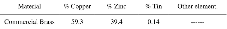
Table 1 Chemical composition of the Brass used in workability tests.
Material % Copper % Zinc % Tin Other element.
Commercial Brass 59.3 39.4 0.14 ---
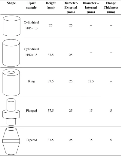
Standard specimens of cylindrical with aspect (H0/D0) ratios of 1.0, 1.5, flanged, tapered and
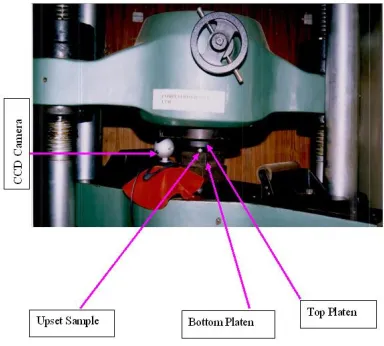
ring of standard dimensions were prepared from the procured rods of 25 mm diameter using a conventional machining operations of turning, facing, drilling and boring. The machined out specimens were shown in Figure 1. Geometries and specifications of specimens for workability tests were given in Table 2. The average surface roughness at the flat and curved surfaces of the specimens was measured as 4 microns and 3 microns respectively. Surf tester was used for the measurement. The upset tests were performed on all the specimens by placing them between the smooth finished flat platens having a 4 microns surface roughness. Extreme care was taken to place the specimens concentric with the axis of the platens. The tests were carried out at a constant cross head speed of 0.5 mm/min using a computer controlled servo hydraulic 100 T universal testing machine (Fuels and Industrial Engineers (FIE), India– UTE model) to obtain different strain paths. The experimental set up of PC based on line video recording system for grid measurement during upsetting was shown in Figure 2.
Ring compression tests were conducted to determine the friction factor ‘m’ for a given set of flat platens. Standard ring compression samples of Outside Diameter (OD): Inside Diameter (ID): Height (H) = 6: 3: 2 (24:12:8 mm) were prepared from the procured rods of 25 mm diameter and were deformed slowly at a ram speed of 0.25 mm/sec on FIE make Compression Testing Machine (CTM- Model-1M 30-0113, 200 T capacity).
[image:4.612.168.477.555.658.2]
Figure 1: Photograph showing the cylindrical samples for upsetting, with different
Table 2: Geometries and dimensions of specimens for workability tests
Shape Upset
sample
Height (mm)
Diameter-External
(mm)
Diameter – Internal
(mm)
Flange Thickness
(mm)
Cylindrical
H/D=1.0 25 25 -- --
Cylindrical
H/D=1.5 37.5 25 -- --
Ring 37.5 25 12.5 --
Flanged 37.5 25 15 5
Figure 2: Experimental set up of PC based on line video recording system for grid measurement during upsetting on 100T computer controlled servo hydraulic UTM
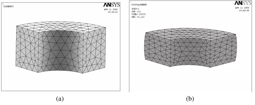
A PC based system consisting of a video camera with an integrated digitizing capacity, 640 X 480 pixels resolution, 256 colour full depth, 20 pictures per second shutter speed, mounted with a magnifying lens was used to record the images of the upsetting process. A 4 X 4 mm square grid was marked at mid height of the standard specimen as shown in figure 3a. Online video images of grid were recorded during the deformation process till the crack initiation site was observed. The distortions of grid from recorded images were analyzed offline. The images were selected at deformation steps of 5% using the software animation shop 3.0 and were transported to paint shop pro 7.0 for further processing to get the enhanced noiseless images of high clarity.
The axial and the circumferential strains were calculated for each element from the measurements obtained according to:
z
ε = ln
0
h
hi and
θ
ε
= ln
0
w wi
Where h0andw0 are theinitial height and width of an element (Figure 3a) respectively, and hi
Figure 3: Schematic diagram of upset tests showing grids for strain measurements
(a) Before deformation (b) after deformation
3. RESULTS AND DISCUSSION
3.1 Friction Factor
The decrease in internal diameter of the ring compression test was plotted against the deformation on Male and Cockcroft [7] calibration curves in increments of 10% deformation. When these ring compression values were fit into calibration curves for the given set of dies, it was found that the friction factor ‘m’ with high finish dies was nearly equal to 0.30, as shown in Figure 4 .The same set of dies was used for upset tests also. Figure 5 shows the ring compression samples before and after deformation.
-60 -40 -20 0 20 40 60 80 100
0 10 20 30 40 50 60 70 80 90
% Deformation
%
D
e
c
re
a
s
e
i
n
I
n
te
rn
a
l
D
ia
m=1.0 m=0.8 m=0.6
m=0.4 m=0.2
m=0.12
m=0.08
m=0.04 m=0.02 m=0
[image:7.612.201.448.452.619.2](a) (b)
Figure 5: Ring compression specimen (OD: ID: H = 6:3:2) (a) Undeformed (b) 30% deformation
3.2 Finite Element Analysis of Ring Compression Test
Finite element analysis of ring compression test was carried out for given frictional condition. Rigid-flexible contact analysis was performed for this process. For such analysis, rigid tools need not be meshed. The ring specimen was meshed with 10-node tetrahedral elements (solid 92 in ANSYS Library). Element size was selected on the basis of convergence criteria and computational time. The program will continue to perform equilibrium iterations until the convergence criteria are satisfied.
The results of the FE analysis for ring compression shows that decrease in the average inside diameter against deformation has a variation of about 10% compared to experimental results. The variation might be due to non uniform friction in the later stages of deformation. Figure 6 shows the undeformed and deformed mesh after 30% deformation of the FEA models of ring compression test (OD: ID: H = 6:3:2) with friction factor (m) = 0.30.
(a) (b)
Figure 6: Quarter FEA model of ring specimen (a) Undeformed (b) 30% Deformed
[image:8.612.100.517.487.660.2]3.3 Load - Displacement Curves
Figure 7 shows the load - displacement curve for brass under friction factor ‘m’ = 0.3 for all the geometry of the specimens. The load requirement increased with increase in the axial displacement of the specimen, it was true for all the specimens. Further an increase in aspect ratio from 1.0 to 1.5; the load required gets reduced for the same amount of deformation. For a fixed diameter, a shorter specimen will require a greater axial force to produce the same percentage of reduction in height, because of the relatively larger undeformed region [16]. Present experimental results were in significance with the above discussion. As per the geometry of the specimen is concerned, to deform the component, tapered specimen required more load than ring and flanged specimens. The experimental loads reveal that geometry of the object also effect the load required for the deformation process.
0.00 100.00 200.00 300.00 400.00 500.00 600.00
0.00 2.00 4.00 6.00 8.00 10.00 12.00 14.00
Displacement,mm
L
o
a
d
,
K
N
[image:9.612.166.442.264.446.2]H/D=1.0 H/D=1.5 Ring Tapered Flanged
Figure 7: Load – displacement curves for Brass in different specimen geometries with friction factor ‘m’=0.30
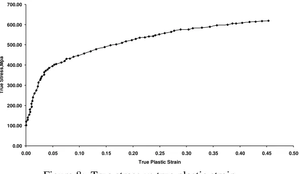
Figure 8 shows the representative plot of
σ
vsε
generated from the upsetting test datacarried out at slow speed with H0/D0 = 1.0 using mirror finished dies. This data was treated
to be material property [17] and used as input for finite element analysis. This curve was fit
into Holloman power law [18-24],
σ
=
K
∗
(
ε
)
n results the flow curve equation asσ
= 8320.00 100.00 200.00 300.00 400.00 500.00 600.00 700.00
0.00 0.05 0.10 0.15 0.20 0.25 0.30 0.35 0.40 0.45 0.50 True Plastic Strain
T
ru
e
S
tr
e
s
s
,M
p
[image:10.612.177.472.68.240.2]a
Figure 8: True stress vs true plastic strain
The specimens of various geometries which were subjected plastic deformation by upsetting up to the fracture initiation were shown in Figure 9. The longitudinal crack and oblique crack were obtained as the two major modes of surface fractures. The mode of fracture depends mainly on the state of stress and the state of strain, both of which in turn depend on the degree of deformation and the slope of the strain path. The longitudinal crack is usually obtained when the axial surface stress is tensile, while the oblique crack is obtained when the axial surface stress is compressive. Cylindrical and ring specimen shows the oblique surface crack while the tapered and flanged shows the longitudinal crack.
H0 /D0 =1.0 H0 /D0 =1.5 (a)
Ring Tapered Flanged (b)
Figure 9: Modes of surface cracking for different specimen geometries.
a) Short (H0 /D0 =1.0)and long (H0 /D0 =1.5)cylindrical specimens
[image:10.612.180.425.398.659.2]3.4 Experimental Strain and Stress analysis using Machine Vision System
Surface strains, circumferential strain (
ε
θ) and axial strain (ε
z) were evaluated for thegeometric mid-sectional grid of the specimens and the results were plotted in Figure 10. Homogeneous deformation corresponds to ideal condition, that is, deformation without
friction or barreling with a constant slope (α) of
θ
ε /
ε
z = -0.5. The line with a slopeθ
ε
/ε
z = -0.5 onε
θ vsε
z plot and which intersects the ordinates atε
θ ≈ 0.3 is an estimateof a fracture line for upsetting test performed on circular cylinders [25]. Though the intercept 0.3 on the ordinate may be approximately correct for steels, it may differ for material to material. Brownrigg et al [26] and H.A. Kuhn et al [27] reported these values of intercepts as 0.29, 0.32, and 0.18 for the 1045 steel, 1020 steel and 303 stainless steel respectively. In the present work this intercept value was observed to be 0.07.
The deviation of slope of the experimentally determined relationship between axial strain
(
ε
z) and circumferential strain (ε
θ), from that corresponding to homogeneous deformationrepresents barreling. This deviation was less when the specimen - die interface friction was
low. In such cases ‘
α
’ was found to be independent ofε
z throughout deformation andsignificant deviation was not observed from the ideal relationship for homogeneous deformation. The strain paths obtained from cylindrical specimens with aspect ratios 1.0 and 1.5 deviated from the line with slope – 0.5, which represents homogeneous deformation. The deviation increased as barreling developed. Flanged and tapered specimen geometries may be regarded as specimens artificially prebulged by machining [28]. Flanged specimen exhibited a strain path similar to that found in axial tension. This is because very little axial compression was applied to the rim during the circumferential expansion caused by compressive deformation of the specimen. Tapered specimen gave strain path with slope somewhere between tension and compression tests [17]. For ring specimen the flow of the material was dominant on the outer periphery compared to the inside periphery of the mid section, the deviation from homogeneous line was observed to be more than the solid cylinder of aspect ratio 1.5.
It is interesting to note that all strain paths obtained from different specimens exhibited nonlinearity from the beginning to the end of the strain path. It is also observed that the slope at a point on the strain path increases as that point moves toward the end of the strain path or the fracture point. This means that at the fracture point, the incremental axial strain
component (d
ε
z) is almost zero, while the incremental circumferential strain component(dεθ) is very high. This change in the slope of the strain path has a great effect on the stress
state at the surface of the specimen. The curve fitting technique was used (because of the scatter in the experimental data for axial and circumferential strains) to obtain a smooth
relationship between the axial strain (
ε
z) and circumferential strain (εθ). This relationship0.00 0.05 0.10 0.15 0.20 0.25
-0.40 -0.35 -0.30 -0.25 -0.20 -0.15 -0.10 -0.05 0.00
Axial strain
C
ir
c
u
m
fe
re
n
ti
a
l
s
tr
a
in
H/D=1.0 H/D=1.5 Ring Flanged Tapered
Homogeneous Deformation Fracture line
Figure 10: Circumferential strainεθas a function of axial strain
ε
zat the equatorialfree surface for Brass (with friction factor ‘m’= 0.30)
Knowledge of the experimental plastic strain history allows experimental evaluation of stress
components during deformation (Appendix B). Effective stress (σ ), and stress components,
circumferential stress (
σ
θ) , axial stress (σ
z) and hydrostatic stress (σ
H) as a function ofeffective strain (ε) calculated from grid measurements of images obtained from Machine
Vision technique for brass of cylindrical samples aspect ratios of 1.0 and 1.5, and also for ring, tapered and flanged were represented in Figure11. In an idealized situation of uniaxial
compression, the circumferential stressσθ, is zero and the axial stress
σ
z is equal to the yieldstress, σ0. Under this condition the hydrostatic component of the stress,
σ
H would be equalto
σ
Z/3 and would always be compressive; a state of instability will never occur inhomogeneous deformation. Hence according to an instability theory of fracture ductile fracture will never occur in homogenous deformation. On the other hand if the friction between the specimen and platens is more, the deformation departed from the homogeneous case, which results barrel develops in the specimen. The tensile circumferential surface stress
component σθ is non zero and the hydrostatic component of stress
σ
H become lesscompressive and in some cases tensile.
The present results referring to Figure 11, the circumferential stress component σθ
increasingly becomes tensile with continued deformation. On the other hand the axial
stressσz, increased in the very initial stages of deformation but started becoming less
compressive immediately as barreling develops. For unfractured specimens the axial
[image:12.612.166.477.83.293.2]occurred both
σ
z andσ
H stress components became less and less compressive asdeformation progresses and become tensile. The hydrostatic stress involves only pure tension or compression and yield stress is independent of it. But fracture strain is strongly influenced by hydrostatic stress [29, 30]. Increase in friction constraint and decrease in aspect ratio caused hydrostatic stress to be tensile and instability starts. As the hydrostatic stress becomes more and more tensile, a state of tensile instability will occur. The transformation in nature of the hydrostatic stress from compressive to tensile depends on the geometry and size of the specimen and the frictional constraint at the contact surface of the specimen with the die block.
From the observation of Figure 11, hydrostatic stress as a function of effective strain, it was concluded that for the same amount of strain hydrostatic stress changes quickly from compressive to tensile under high friction conditions and for small aspect ratios. The nature of hydrostatic stress on the rim of the flanged specimen was tensile from the beginning of the deformation while the axial stress on the rim was almost zero and the circumferential stress coincides with the effective stress of the material. The nature of hydrostatic stress for ring, tapered specimens lie between the regions of cylindrical specimen with aspect ratio 1.5 and the flanged specimens. For the brass, the extent of deformation from instability to fracture is small. However this post instability strain to fracture can be increased by changing the microstructure via proper heat treatment. Both normal and shear type of fracture were observed during metal experiments. Normal fracture was observed for the flanged and tapered samples due to presence of tensile axial stress at fracture, while shear fracture was observed for the rest of the specimens.
-600.00 -400.00 -200.00 0.00 200.00 400.00 600.00 800.00
0.00 0.05 0.10 0.15 0.20 0.25 0.30 0.35
Effective Strain
S
tr
e
s
s
,M
P
a
Effective Stress,MPa
Axial Stress,MPa
Circumferential Stress,MPa
Hydrostatic Stress,MPa
-600.00 -400.00 -200.00 0.00 200.00 400.00 600.00 800.00
0.00 0.05 0.10 0.15 0.20 0.25 0.30 0.35 0.40 0.45
Effective Strain
S
tr
e
s
s
,M
P
a
Effctive Stress
Axial Stress
Circumferential Stress
Hydrostatic Stress
(b)
-600.00 -400.00 -200.00 0.00 200.00 400.00 600.00 800.00
0.00 0.05 0.10 0.15 0.20 0.25 0.30 0.35 0.40
Effective Strain
S
tr
e
s
s
,M
P
a
Effective Stress,MPa
Axial Stress,MPa
CIrcumferential Stress,MPa
Hydrostatic Stress,MPa
-50.00 0.00 50.00 100.00 150.00 200.00 250.00 300.00 350.00 400.00
0.00 0.05 0.10 0.15 0.20 0.25 0.30
Effective Strain S tr e s s ,M P
a Effective Stress,MPa
Axial Stress,MPa Circumferential Stress,MPa Hydrostatic Stress,MPa (d) -300.00 -200.00 -100.00 0.00 100.00 200.00 300.00 400.00 500.00 600.00
0.00 0.05 0.10 0.15 0.20 0.25 0.30 0.35
[image:15.612.93.524.69.606.2]Effective Strain S tr e s s ,M P a Effective Stress,MPa Axial Stress,MPa Circumferential Stress,MPa Hydrostatic Stress,MPa (e)
Figure 11: Effective stress (σ ), stress componentsσθ, σz and σH as a function of
Effective strain (
ε
) for copper under low friction condition (Friction factor ‘m’=0.30) (a)H0/D0 = 1.0, (b) H0/D0 = 1.5, (c) Ring, (d) Flanged, (e) Tapered.
4. FINITE ELEMENT MODELING
Finite element analysis of deformation behavior of cold upsetting process was carried out for cylindrical specimens with aspect ratios of 1.0 and 1.5 and also for ring, tapered and flanged specimens. Since computers with high computational speed are now available in the market at relatively cheaper cost, the time of computation is not a major constraint for solving the problems of small sized 3-D models. Further, the tetrahedral elements can easily be accommodated in any shape [31]. This reduces the number of iterations and steps to be solved. Owing to these facts the present problem was solved using 3-D model. The analysis can also be extended to non axisymmetric problems using a full 3-D model. In the present analysis, quarter portion of 3-D model was considered with symmetric boundary conditions.
Rigid-flexible contact analysis was performed for the forming process. For such analysis, rigid tools need not be meshed. The billet geometry was meshed with 10-node tetrahedral elements (solid 92 in ANSYS Library). Element size was selected on the basis of convergence criteria and computational time. Too coarse a mesh may never converge and too fine a mesh requires long computational time without much improvement in accuracy. The program will continue to perform equilibrium iterations until the convergence criteria are satisfied. It will check for force convergence by comparing the square root of sum of the squares (SRSS) of the force imbalances against the product of the SRSS of the applied loads with a tolerance set to 0.005. Since the tolerance value in the program is set to 0.5%, the solution will converge, only if the out of balance force is very small leading to more accurate results.
Material models were selected based on the properties of the tooling and billet materials. Due to high structural rigidity of the tooling, only the following elastic properties of tooling (H13 steel) were assigned assuming the material to be isotropic [32]. Young’s Modulus E =
210 GPa and Poisson’s ratio υ = 0.30. For billet material model selected is isotropic Mises
plasticity with E = 110 GPa, υ = 0.375 and plastic properties obtained from Hollomon power
law equation. As the nature of loading is non-cyclic, Bauschinger effect could be neglected and the non-linear data was approximated to piecewise multi linear with 10 data points. Care is taken that the ratio of stress to strain for first point equals to Young’s modulus of copper. The material was assumed to follow the Isotropic hardening flow rule. Suitable elastic properties were also assigned for the material chosen for analysis. As the experiments were conducted at room temperature, the material behavior was assumed to be insensitive to rate of deformation [33- 35].
geometric entity in space that senses and responds when one or more contact elements move into a target segment element.
5. VALIDATION OF FEA RESULTS
Figure 12 shows the specimen before deformation. There was zero friction at metal-die contact and no apparent bulging; the deformation can be treated as homogeneous, figure 13. The variation in the values of radial diameter at 50% deformation obtained from finite element analysis and calculated values from volume constancy condition is 0.7% [37]. This small variation may be neglected in non linear finite element analysis such as in large deformation / metal forming applications.
The profiles of radial displacement and total strain distribution for all the specimens were
shown in figures from 14 to 17. The hydrostatic stress (
σ
H) profiles for Cylindrical(a) (b)
(c) (d)
[image:18.612.96.528.81.681.2](e)
Figure 12: FEA modeled Undeformed specimens (a) Cylindrical specimen, Ho/Do =1.0
(a) (b)
Figure 13: Cylindrical specimen (Ho/Do =1.0) at 50% deformation under zero friction
(a) Radial Displacement (b) Total Strain Distribution
(a) (b)
Figure 14: Cylindrical specimen (Ho/Do =1.5) at the point of fracture initiation (32%
deformation) under friction factor ‘m’=0.3
[image:19.612.98.524.366.559.2](a) (b)
Figure 15: Ring specimen at the point of fracture initiation (30% deformation) under friction factor ‘m’=0.3 (a) Radial Displacement (b) Total Strain Distribution
(a) (b)
[image:20.612.96.526.367.562.2](a) (b)
[image:21.612.205.403.336.481.2]Figure 17: Flanged specimen at the point of fracture initiation (24% deformation) under friction factor ‘m’=0.3 (a) Radial Displacement (b) Total Strain Distribution
Figure 18: Hydrostatic stress at the point of fracture initiation (27% deformation) of
Cylindrical specimen (Ho/Do =1.0).
Figure 19: Hydrostatic stress at the point of fracture initiation (32% deformation) of
[image:21.612.209.400.547.687.2]Figure 20: Hydrostatic stress at fracture initiation (30% deformation) of Ring specimen
Figure 21: Hydrostatic stress at fracture initiation (27% deformation) of Tapered specimen.
[image:22.612.201.409.528.688.2]Table 3: Comparison of experimental and FEA results for Brass
Stress, MPa Specimen
geometry
θ
σ (circumferential
σ
z(axial)σ
H(hydrostatic)H/D=1.0 301 (296) -341 (-347) -15 (-17)
H/D=1.5 280 (278) -403 (-405) -42 (-42)
Ring 376 (353) -303 (-327) 16 (09)
Flanged 384 (380) 07 (09) 131 (131)
Tapered 376 (379) -130 (-175) 67 (68)
Note: Numbers inside the parenthesis indicates the experimental values
6. CONCLUSIONS
1. Friction factor ‘m’ was determined experimentally for given set of dies.
2. Inverse FEA modeling and analysis was successfully performed from the
experimentally obtained friction factor values.
3. Vision system was successfully employed in the measurement of grid distortion at
equatorial surface for the analysis of stress components. Implementation of Vision system reduced the extent of experimentation.
4. The workability limit for brass has been determined experimentally. The workability
limit is a useful tool in the design and manufacturing stages of any product.
5. At the beginning of deformation axial compressive stress increased in magnitude but as
the deformation progress the magnitude reduced. Hydrostatic stress also reduced in magnitude as the deformation increased. Increase in friction constraint and decrease in aspect ratio caused hydrostatic stress to be tensile.
6. The nature of hydrostatic stress on the rim of the flanged specimen is found to be
tensile.
7. The nature of hydrostatic stress for ring, tapered specimens lie between the regions of
cylindrical with aspect ratio 1.5 and the flanged specimens.
8. The time history data is useful in designing the intermediate dies for new materials with
quite a small number of deformation experimental trials reducing the lead-time of design cycle.
9. Results obtained by finite element analysis closely matched with the experimental
ACKNOWLEDGEMENTS
The authors thank the AICTE, New Delhi for their financial support under AICTE – CAYT scheme (File No:1-51/FD/CA/(19) 2006-2007) and also the Departments of Metallurgical and Civil Engineering, AU College of Engineering, Andhra University Visakhapatnam for providing necessary support in conducting the experiments.
Appendix A: Experimental Strain Path equations
Equations obtained by the best fit technique for the experimental strain components of different strain paths were tested by compression.
S No Condition Strain path equation
1. H0/D0=1.0, m=0.30 εθ = 0.3701 εz 3 + 0.9116 εz 2 – 0.5606 εz
2. H0/D0=1.5, m=0.30 εθ = -0.6628 εz 3 + 0.1807 εz 2 – 0.5284 εz
3. Ring, m=0.30 εθ = -1.8429 εz 3 – 0.075 εz 2 – 0.5367 εz
4. Tapered, m=0.30 εθ = -8.1524 εz 3 + 0.105 εz 2 – 0.763 εz
5. Flanged, m=0.30 εθ = -247.96 εz 3 – 10.863 εz 2 – 2.1981 εz
Appendix B: Stress Components as a function of the slope of the strain path (α)
The Levy-von Mises yield criterion can be written in terms of principal stresses as
σ = 3J2 = [σθ2+ σz2-σθσz]1/2 --- (1)
Because the transverse stress component σr is zero on the free surface. Here J2 is the
second invariant of the stress deviator.
The plastic strain increment at any instant of loading is proportional to the instantaneous stress deviator, according to the Levy-Von Mises stress strain relationship: i.e.
dεij =σij' dλ --- (2)
where dλ is non negative constant which may vary throughout the loading history.
For σr= 0, equation (2) yields
θ θ θ σ σ σ σ ε ε − − = z z z d d 2 2 or 2 2 1 + + = α α σ σθ z --- (3) where z d d ε ε α = θ
is a parameter which can be determined by experimental measurements of
specimen, figure 9. Substituting equations (3) and (1) gives the following expression for σθ
andσz.
2 / 1 2 2 2 1 2 2 1 1 − + + + + + − = α α α α σ
σz ---(4)
And
+ + = α α σ σθ 2 2 1
z ---(5)
By convention, compressive stresses are negative, thus the lower sign in equation (4) is used
in evaluatingσz. σ denotes the effective flow stress for an isotropic material for the
appropriate effective strain ε at the free surface.
In terms of the principal strain increments
(
2 2)
1/23 2
z
z d d
d d
dε = ε θ + ε + εθ ε ---(6)
where, the incompressibility condition dεr +dεθ +dεz =0 has been used.
The effective strain at the free surface from equation (6) is given by
ε =
∫
εzdε0 = 3
2
(
)
z d z ε α α
ε 1/2
0
2
1
∫
+ + ---(7)where the integration can be performed along the strain path provided the principal axes of the strain increment do not rotate relative to element.
The equations (4),(5) and (7), will enable us to calculate the stresses and effective strains on the geometric centre of the bulge surface (shown in figure 5) and are identical to the
equations derived by Kudo and Aoi and David et al [38, 39]. Theoretically, α may take any
value between -∞ and +∞ but there is no real value of α for whichσθor σzwould increase
with out bounds. In the present experimental situation the range ofα is limited to -2 to -1/2.
As α increases, the tensile stressσθ increases but the hydrostatic stress σH =
(
σθ +σz)
/3,REFERENCES
1. Jolgaf, M., Hamouda, A.M.S., Sulaiman, S., Hamdan, M.M, 2003, Development of a
CAD/CAM system for the closed–die forging process, J of Material Processing Technology, 138: 436-442.
2. Rajiv Shivpuri, 2004, Advances in Numerical Modeling of Manufacturing process,
Application to steel, Aerospace and Automotive Industries. Trans. Indian. Inst. Metals, 57: 345-366
3. Taylan Altan., Hannan, D A N, 2002, Forging: Prediction and Elimination of Defects in
cold forging using process simulation, The Engineering Research Center for Met shape manufacturing. http.www.ercnsm.org. 2002.
4. Victor Vazquez., Taylan Altan., 2000, New Concepts in die design–physical and
Computer Modeling applications. J of Materials Processing Technology, 98: 212 – 223.
5. www.forging.org
6. Kunogi, 1954, Reports of the scientific Research Institute, Tokyo.30: 63.
7. Male, A. T., and Cockcroft, M.G, 1964-65, A Method for the Determination of the
Coefficient of Friction of Metals under Conditions of Bulk Plastic Deformation. J. Inst. of Metals. 93: 38.
8. Altan T Male, and Vincent Depierre, 1970, Transactions of the ASME J of Lubrication
Technology, July 1970: 389 – 397.
9. Samantha S.K, 1975, Effect of friction and specimen geometry on the ductile fracture in
upset. Institute of Engineering Materials and Technology. Transactions of ASME, Jan 1975: 14-20.
10.Santos, Duarte, D. J.F., Anareis, Rur Neto, Ricardo Paiva, Rocha, A.D, 2001, The use of
finite element simulation for optimization of Metal forming and tool design. J of Material Processing Technology. 119: 152 -157.
11.Kobayashi, S., Oh, S.I. and Altan T, 1989, Metal forming and Finite Element Method,
Oxford University Press, New York.
12.Lee, C.H., and Kobyashi, S, 1973, New solutions to rigid plastic deformation problems
using a matrix method. J of Engineering for Industry Trans. of ASME. 95: 865.
13.Jackson, J.E, J.r., and Ramesh, MS, 1992, The rigid plastic finite element method for
simulation of deformation processing, Numerical Modeling of Material deformation Processes. Springer-Verlag, London, pp 48 – 177.
14.Bathe K.J, 1996, Finite Element Procedures- Prentice – Hall, pp 622.
15. ASM Hand Book, 1996, Forming and Forging, ASM International.
16.George E. Dieter, 1928, Mechanical Metallurgy- McGraw-Hill Book Company, London
17.Gouveia, B.P.P.A, Rodrigues, J.M.C. and Martins, P.A.F, 1996, Fracture Predicting In
Bulk Metal Forming. Int. J. Mech. Sci.38: 361-372
18. Ungair, T., Gubicza, J.,Ribairik, G. and Borbeily, A., 2001, J. of Applied
Crystallography. 34: 298
19.Iwahashi, Y., Horita, Z., Nemota, M. and Langdon, T.G., 1998, Metall Mater Trans A
29: 2503
21.Erik Parteder and Rolf Bunten., 1998, Determination of flow curves by means of a compressive test under sticking friction conditions using on iterative finite-element procedure, J. of materials processing Technology. 74:227-233
22.Hollomon, J. H., 1945, Transactions, AIME. 162: 268
23.Wei Tong., 1998, Strain Characterization of propagative deformation bands. J of the
mechanics and physics of solids. 46 (10):2087 – 2102
24.Johs A. Bailey., 1969, The plane strain forging of Aluminum and An Aluminum alloy at
low strain rates and elevated temperatures. Int J of Mechanical Science. 11: 491 – 507.
25.Samantha, S.K., 1975, Effect of friction and specimen geometry on the ductile fracture in
upset. Institute of Engg Materials and Techn., Transactions of ASME. 14:20
26. Brownrigg, A., Duncan, J.L. and Embury, J.D., 1979, Free Surface Ductility of Steels in
Cold Forging, Internal Report, McMaster University, Hamilton, Ontario, Canada.
27.Kuhn, H.A., Lee, P.W. and Erturk, T., 1973, A Fracture Criterion for Cold Forming, J of
Engg Materials and Techn, Transactions of the ASME: 213 – 218
28.Erman, E., Kuhn, H.A., and Fitzsimons, G., 1983, Novel test specimens for workability
testing, in compression testing of Homogeneous Materials and Composites. ASTM STP, 808: 279
29.George E Dieter., 1988, Mechanical Metallurgy, McGraw-Hill Book Company-London,
pp.45-46
30.B. Rozzo, P., Deluca, B. and Rendina, R., 1972, A new method for the prediction of
formability limits in metal sheets, Sheet Metal Forming and Formability: Proceedings of
the 7th biennial Conference of the International Deep Drawing Research group
31.Wu, W.T., Jinn, J.T. and Fischer, C.E.: Scientific Forming Technologies Corporation,
Chapter15.
http://www.asminternational.org/Template.cfm?Section=BrowsebyFormat&template=Ec ommerce/FileDisplay.cfm&file=06701G_ch.pdf
32.http://www.matweb.com
33.Kobayashi S., 1970, Deformation Characteristics and Ductile Fracture of 1040 Steel in
Simple Upsetting of Solid Cylinders and Rings, J of Engineering for Industry, Trans ASME, Series B, May 92 (2): 391 -399
34.Lee, C.H. and Kobayashi, S., 1973, New Solutions to Rigid-Plastic Deformation
Problems Using a Matrix Method. Journal Eng. Ind. (Trans. ASME), 95: 865
35.Zeinkiewiez, O.C., 1984, Flow Formulation for Numerical Solution of Forming Processes
in J.F.T. Pittman et al. (Eds), Numerical Analysis of Forming Processes, Wiley. New York, pp.1- 44
36.Ansys 8.0 Reference Manual.
37. Syed Kamaluddin, J Babu Rao, MMM Sarcar and NRMR Bhargava, 2007, Studies on
Flow Behavior of Aluminum Using Vision System during Cold Upsetting. Met and Mater. Trans. B, 38 B: 681-688.
38.Kudo, H, and Aoi, K., 1967, Effect of Compression Test Condition Upon Fracturing of a
Medium Carbon Steel – Study on Cold – Forgeability Test; Part II, Journal of the Japan Society of Technical Plasticity, 8:17-27
39.David, W, Manthey, Dr. Daeyong Lee, Rebecca M. Pearce, 2005, The Need for Surface