Distributed state space generation for graphs up to isomorphism

(1)

Distributed State Space Generation

for Graphs up to Isomorphism

Gijs Kant

24 August 2010

Master’s thesis

Department of Computer Science

Graduation committee:

(2)

(3)

Summary

In order to achieve reliability of systems, formal verification techniques are required. We model systems as graph transition systems, where states are represented by graphs and transistions between states are defined by graph transformation rules. For formal verication, often the state space of the system has to be generated, i.e., the set of all reachable states. The main problem with generating the state space is its size, which tends to grow exponentially with the size of the modelled system. This results in enormous computation time and memory usage already for relatively small systems. Recent developments in hardware design aim towards multi-core and multi-processor architectures. In order to benefit from these we require distributed tools: the task of state space generation needs to be split up into subtasks that can be distributed to multiple cores, called workers.

In this report we present a tool fordistributed state space generationfor graph-based systems. The tool uses LTSMIN[23]for efficiently distributing the states over the workers and for storing the state space, and instances of GROOVE[28]for computing successor states by applying graph transformation rules. Because LTSMINuses fixed sized state vectors to represent states, a serialisation from graphs

to state vectors and its reverse are required. We define two such serialisation functions: one that partitions the graph by its nodes (node vector) and one that uses edge labels to partition the graph (label vector).

In graph transformation systems a powerful symmetry reduction can be achieved by using isomorphismchecking[27]. Isomorphic states can be merged, resulting in a reduced transition system that is bisimilar to the transition system without reduction, which implies that they satisfy the same semantic properties[29]. In our distributed tool we compute a canonical form for each computed successor graph, which enables us to also distribute the isomorphism reduction to the workers. For computing canonical forms, BLISS (described in[16]) is used together with a conversion that is

needed because GROOVEuses a slightly different graph formalism (edge labelled graphs) than BLISS

(coloured graphs) does.

We have performed experiments to investigate the time and memory performance of the distribu-ted tool, based on LTSMIN, with the two different serialisation functions, compared to the sequential version of GROOVE for three different case studies. The experiments show that the node vector encoding is better than the label vector encoding both in memory usage and execution time.

The distributed setup with the node vector serialisation results in orders of magnitude less memory usage than sequential GROOVEfor the very symmetric cases. This is suprising because the storage in

GROOVEis optimised for graphs, storing only the differences (deltas) between state graphs instead of

the complete graphs themselves.

The execution time for LTSMINwith one core is much worse than that of GROOVE, because GROOVE

uses a canonical hashcode, which often prevents that isomorphism checking has to be used, and some kind of partial order reduction for graph transition systems that is not applicable in the distributed setting. Also, the conversion to coloured graphs, needed for computing canonical forms using BLISS,

blows up the size of the graphs. However, for the larger models the distributed solution scales well. For all reported case studies there are start graphs for which GROOVEruns out of memory or is not

capable of finishing within the time limit, while the distributed tool still can generate the state space. In one of the cases a speedup of 16 is achieved with 64 workers in the largest case for which also GROOVEcould generate the state space within the time limit. For the very symmetric cases most of the time is spent on isomorphism checking in GROOVE. In the distributed setting, the speedup is explained

by the time spent on canonical form computation that decreases linearly as the number of workers increases. As the number of workers increases, however, the communication overhead also grows.

(4)

(5)

Introduction

Computer systems and software are everywhere around us. Internet applications and databases are widely used for communication and administrative tasks. We are more and more dependent on the availability of such systems for economic transactions, communication, etc. Computer systems are also used in safety-critical situations, for controlling power plants, airplanes, cars, etc. These systems become more and more complex, especially with the ongoing trend towards distributed systems and parellel software. Therefore we need reliable systems and for that we need techniques to verify systems and to assist in building reliable, dependable systems.

In software engineering there are several ways to establish correctness and reliability of the software product. We consider one of them, which is to formally specify the behaviour of the system and verify that the system satisfies some set of formal properties, e.g., that it is free of deadlocks and that no illegal state can be reached. The properties can be expressed as formulae in a temporal logic, such as Computational Tree Logic (CTL) or Linear Temporal Logic (LTL). Verifying that a specification satisfies such a formula is calledmodel checking. This kind of verification is usually done by exploring thestate spaceof the specified system, i.e., the set of all reachable states (from some given initial state). The state space is represented as aLabelled Transition System(LTS), where each transition represents an action that is possible from a certain state and to which state the action leads. Checking correctness properties can be done while generating the LTS (on-the-fly) or afterwards if the LTS is stored somewhere.

We model systems asgraph transformation systems, wherestatesare represented bygraphsand transistionsbetween states are defined bygraph transformation rules. Modelling systems as graph transformation systems has certain advantages. Modelling states as graphs provides an elegant way of expressing entities and relations between entities. Graph transformation systems have a solid formal basis, the semantics of graph transformation rules are well defined. Various tools exist that support graph-based modelling of systems. For instance, the tool GROOVE[28]can be used for graph-based

model checking[27]. In GROOVE, directed edge labelled graphs are used to model states. See, e.g., [12]for examples of modelling and analysis using GROOVE. In Chapter 2 the basic concepts related to

graphs and graph transition systems are presented.

The main problem with model checking is the size of the transition system, which tends to grow exponentially with the size of the specified system. This results in enormous computation time and memory usage already for relatively small systems. Many kinds of techniques have been developed and are still being developed to try to cope with this complexity of model checking. There are very powerful reduction techniques that reduce the size of the transition system without changing its semantic properties, such as Partial Order Reduction (see, e.g.,[2]).

Recent developments in hardware design aim towards multi-core and multi-processor architec-tures. In order to benefit from these we require distributed tools: the task of state space generation for graph transformation systems needs to be split up into subtasks that can be distributed to multiple cores or machines, calledworkers. The algorithms in GROOVEare written to run on one machine. As

far as we know, no other tools are currently available that provide distributed state space generation for graph transformation systems. Tools already exist for distributed state space generation for states

(8)

2 Introduction

modelled as vectors of data which, however, cannot be used directly for graphs. One of these is the LTSMINtoolset[23].

In this report we present a tool fordistributed state space generationfor graph-based systems. The tool uses LTSMINfor efficiently storing the state space and distributing the states over the workers, and instances of GROOVE for computing successor states by applying graph transformation rules.

Because LTSMINuses fixed sized state vectors to represent states, a serialisation from graphs to state

vectors and its reverse are needed for using LTSMINto communicate graphs. We define two such

serialisation functions for graphs: one that partitions the graph by its nodes (node vector) and one that uses edge labels to partition the graph (label vector).

In state space generation, there are also techniques for symmetry reduction, i.e., grouping of ‘symmetric’ states. Particularly for graph transformation systems a powerful symmetry reduction can be achieved by usingisomorphismchecking[27]. Isomorphic states are structurally equivalent, but the nodes of the graph can have different identities. Because application of transformation rules is based on matching, i.e., finding a subgraph isomorphism, isomorphic states give rise to equivalent transitions with equivalent target states. Therefore, if two states are isomorphic, they are considered to represent the same state and only one of them has to be stored. The resulting reduced transition system is bisimilar to the transition system without reduction, which implies that they satisfy the same properties[29]. This reduction can be established in two ways: (a) when encountering a new state we can search in the set of visited states for an isomorphic state; or (b) we can compute a canonical form of the graph and store that canonical form. A canonical form of a graphGis a graph that is isomorphic toG, such that for a graphH, the canonical forms ofGandHare equal if and only ifG andHare isomorphic. By definition a set of isomorphic graphs has only one canonical form, which serves as unique representative of that set.

In our distributed tool we compute a canonical form for each computed successor graph, which enables us to also distribute the isomorphism reduction to the workers. Canonical forms for coloured graphs, a slightly different graph formalism from the edge labelled graphs used in GROOVE, can be

computed by BLISS(described in[16]), which is an improved version of NAUTY(described in[19]).

In Chapter 4 the theory behind these tools is described and a conversion from edge labelled graphs to coloured graphs is presented. An extensive survey of different methods for computing canonical forms is given in[17].

We have performed experiments with several rule systems to compare the distributed setup, based on LTSMIN, to the existing sequential version of GROOVE. The results show that a significant speedup

and much better memory usage are achieved by the distributed approach compared to GROOVE.

This report is organised as follows. In the next section we discuss related work. Chapter 2 introduces the concepts and definitions used in the report. The architecture of the distributed state space generation tool and the relation between LTSMIN, GROOVEand BLISSare described in Chapter 3. The algorithms behind graph canonizer BLISSand how BLISScan be applied to edge labelled graphs

are described in Chapter 4. We describe the graph serialisations and formally demonstrate their correctness in Chapter 5. The experiments and results are presented in Chapter 6. Chapter 7 concludes the report and contains suggestions for future work.

1.1

Related Work

(Distributed) Graph transformation. Some work has already been done on parallelisation of graph transformation by parallelising graph matching, see[4]. Pattern matching and rule application are parallelised by distributing the storage and updating of the rule match network, the so called retenetwork. However, that work is aimed at performing linear graph transformation rather than generating a complete state space. In that case isomorphism reduction is not an issue.

Distributed state space generation. Several tools exists for distributed model checking based, such as distributed versions of the model checker SPIN_[18, 3_]and the tool LTSMIN[5, 23]. SPIN

uses a process modelling language (Promela) as input. In[30]a serialisation of graph grammars to Promela models (used in SPIN) is reported, but the performance (with normal SPIN) is worse than that of GROOVE. LTSMINis very modular by design and supports multiple language modules (for

input) and multiple model checking tools (for verification). That is why we choose to use LTSMIN,

(9)

1.1 Related Work 3

Graph isomorphism. Subgraph matching is known to be a NP-complete problem (Problem GT48 in[11]). For isomorphism checking it is not known if the time complexity is in P or if the problem is NP-complete. It is believed not to be in P[34].

Many algorithms exists that can check if two graphs are isomorphic. Ullmann[33]presented a search tree based algorithm for finding graph or subgraph isomorphisms between two graphs. Messner & Bunke[21, 22]made an optimised version for large graphs. The graph matching algorithms by Cordella et al.[6, 7, 8]also aim at isomorphism checking for pairs of graphs. They use heuristics and efficient data structures that are optimed for matching large graphs. Foggia, Sansone, and Vento compare four one-to-one isomorphism checking algorithms to NAUTY, a tool that computes canonical forms[10]. For many cases NAUTYperforms comparable to these algorithms or better. For some cases NAUTYperforms worse or is unable to find an answer, whereas some other algorithms are able to find an answer for all test cases.

Computing canonical forms. The NAUTYprogram by McKay[20]is able to produce a canonical

form for directed coloured graphs, which can be used to test for isomorphism between graphs. The algorithm of McKay for computing the canonical form is described in[19]and will be explained in Section 4.2.

The complexity of the algorithm of McKay has been analysed by Miyazaki[24]. Miyazaki shows that NAUTYhas an exponential worst case complexity. For some 3-regular graphs (for which canonical

labellings can be computed in polynomial time, see_[1_]) NAUTYhas an exponential lower bound.

However, in practice the average computation time is much better.

Optimisations of McKay’s algorithm for large and sparse graphs have been done by Junttila & Kaski[16]in the tool BLISS[15]. In experiments BLISSis shown to be faster than NAUTYfor large and

sparse graphs. It uses datatypes that allow more efficient storage and searching than the adjacency matrix that is used in NAUTY. Also other certificates for nodes in the search tree are used and the

heuristics for pruning certain subtrees of the search tree are further optimised.

Using canonical forms in model checking. The tool NAUTYhas been used in model checking of

systems specified in B by the tool PROB[32, 31]. The states of the B model are translated to edge

labelled graph representations. These are again converted to a coloured graph representation and compared using NAUTY. In[32]a version of the NAUTYalgorithm is used that is adapted to work for

edge labelled graphs, but the search tree pruning optimisations of NAUTYare left out. In[31]on the

contrary a conversion from edge labelled graphs to vertex coloured graphs is used in combination with the orignal NAUTYalgorithm. In both approaches the states of the B model are converted to

(10)

(11)

2

Graph-Based Verification

In this chapter we define concepts that will be used troughout the report, such as graphs, isomorphism of graphs, graph transformation, and graph transition systems.

2.1

Graphs

Agraphis a structure that consists of a set ofvertices(ornodes) and a set ofedges(orarrows) between vertices. There are many different kinds of graphs, with and without labels or colours, with directed or undirected edges, and with only binary orn-ary edges. We usedirected labelled graphs, to be defined shortly hereafter. We assume a fixed ordered set of edge labelsLEand a fixed ordered set of vertex labelsLV. Vertex labels are used fortypesandflags, which are unary edges, i.e., edges that are connected to exactly one vertex. A vertex can have at most one type and arbitrary many flags. We also use special nodes representing primitive values, elements of the setVal=Int_∪Bool_∪String_∪Double. We denote the set of types asT=_{Int,Bool,String,Double_}. We write the primitive values as tuples, e.g.,〈Int, 1〉,〈Bool,true〉and use functionstype:T_×Val_→T andval:T_×Val_→Valfor the type repectively value of the value nodes. E.g.,type(_〈Int, 1〉) =Intandval(_〈Int, 1〉) =1.

Let us define formally what we mean by directed labelled graphs.

Definition 2.1(Directed labelled graph). Adirected labelled graph Gis a tuple〈V,E,c_〉with a finite nonempty ordered set of verticesV = (0, 1, . . . ,n₋1)with vertices represented by natural numbers in the range[0..n−1], a set of ordered tuplesE_⊆V_{× L}_E_×V representing the binary edges, and a colouring functionc:V_{→ P}(_L_V)_∪Valthat associates a set of vertex labels or a primitive value with each vertex. The edges have associated source and target functionssrc,tgt:E→V and label functionlab:E→ LE. The class of directed labelled graphs is denotedGL.

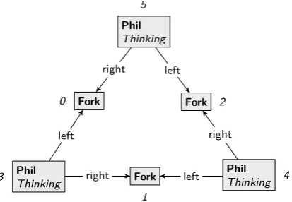
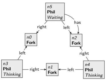
Example 2.2. As an example throughout the report we use thedining philosophers problem, essentially a problem of mutual exclusion. The problem can be briefly described as follows. A number of philosophers (we use three for the example) is sitting around a table, where they are about to eat spaghetti. To the left and to the right of each philosopher there is a fork, i.e., each fork is shared by two philosophers. Each philosopher needs two forks to be able to eat spaghetti. Philosophers are eitherthinking, trying to acquire forks (waiting), oreating. Figure 2.1 depicts the start state of the problem. The square boxes denote nodes in the graph, with a bold face label for its type and italic face labels for flags. In the figure the nodes are numbered 0..5. These so callednode identitiesare shown outside of the nodes or inside the box asn0,n1, etc, which is the notation that is being used in GROOVE. Node identities are only needed to write down the graph on paper in a textual form and

for storing them in computer memory. The arrows denote the edges between nodes. The edges are directed, which means that, e.g., the edge(5,right, 2)has node 5 as source and node 2 as target.

(12)

6 Graph-Based Verification

Phil

Thinking

Fork

Fork Phil

Thinking

Fork

Phil

Thinking 0

1

2

3 4

5

right left

left right

[image:12.595.193.400.74.217.2]

left right

Figure 2.1: Example graph representing a state in the dining philosophers problem.

2.2

Graph Transformation

Graphs can be transformed using graph transformation rules. Without going in to details, we will explain here the basic concepts in graph transformation that are necessary in the context of this report. Graph transformation is defined category theoretically in terms of morphisms and pushouts. A graphmorphismis a structure preserving mapping from elements in one graph to elements in another graph. This mapping can be a partial mapping. If the mapping is a bijection it is an isomorphism. A pushoutis a formal definition of the result of combining morphisms. The rule is applied to a graph that is called thehost graph. A detailed description of graph transformation, morphisms, pushouts and graph transition systems can be found in, e.g.,[9].

A graph transformation rule consists of three parts:

Left Hand Side (LHS) Thereaderanderaserelements of the rule. These are the elements that are used for finding amatch, which is a morphism from the LHS of the rule to the host graph. The eraserelements will be deleted from the host graph when the rule is applied.

Right Hand Side (RHS) Thereaderandcreatorelements of the rule. There is a morphism between the reader elements of the LHS to the reader elements of the RHS. Thecreatorelements are added to the host graph when the rule is applied.

Negative Application Condition (NAC) Theembargoelements and (some of the)readerelements of the rule. There is a morphism between the reader elements of the NAC to (part of) the reader elements of the NAC. If a match (extending the match between host graph and LHS) can be found from the NAC to the host graph, then the rule isnotapplicable.

The transformation takes place in three steps: i)matchingthe reader and eraser elements (the LHS) of the rule to (a subgraph of) the host graph, the graph on which the transformation takes place (i.e., finding a morphism between the host graph and the LHS), ii) trying to extend the match between host graph and LHS with a match between host graph and the NAC, and iii)applyingthe change that is specified by the rule if a match is found for the reader elements, but not for the NAC. Rule application in GROOVE is done in a Single Pushout (SPO) manner. The most important

consequence of that is that when a node is removed also attached edges are removed automatically. We will not further explain pushouts here. See, e.g.,[9]for a more detailed account.

In GROOVEthe three parts of rule are combined in a single graph representation. There the black parts of the rule form thereaderelements, the blue dashed parts form theeraserelements, the green thick elements are thecreatorelements, and the red thick dotted elements are theembargoelements.

Example 2.3. Figure 2.2 shows a graph transformation rule in the two different representations. The tranformation rule looks in the host graph for a philosopher node and the adjacent fork node to the left of the philosopher (LHS) such that no philosopher already has taken the fork (NAC). The rule adds ahaslabel between the philosopher and the fork representing that the philosopher has taken the fork (RHS). Between the LHS, RHS, and NAC there are implicit morphisms, i.e., nodesn0andn1

(13)

2.2 Graph Transformation 7

n1

Fork

n0

Phil

−Thinking

+Waiting

n2

Phil

left has

has

(a)ThepickupLeftrule in the single graph represenation used in GROOVE.

n1

Fork

n2

Phil

has

NAC

n1

Fork

n0

Phil

−Thinking

left

LHS

n1

Fork

n0

Phil

+Waiting

left

has

[image:13.595.83.509.98.322.2]

RHS (b)ThepickupLeftrule as three graphs with implicit morphisms.

Figure 2.2: Example graph transformation rule:pickupLeft.

n4

Phil

Thinking n5

Phil

Waiting

n1

Fork

n2

Fork

n0

Fork

n3

Phil

Thinking left

right left

left has

right

[image:13.595.202.390.517.658.2]

right

(14)

When applying the rule to the graph in Figure 2.1, there are three possible resulting states, because the rule can be applied to three pairs of philosopher and fork nodes. The three resulting states are isomorphic, i.e., only the node identities are different. Isomorphism will be defined in Section 2.4. One of the resulting state graphs is in Figure 2.3.

2.3

Graph Transition Systems

Given a start graph and a set of graph transformation rules (also called a graph grammar), we can compute all states reachable from the start state. This results in a graph transition system, as described in[27]. We writeG for a class of graphs, e.g. directed labelled graphs,Rfor the class of graph transformation rules that can be applied to graphs inG, andLR for the class of transition labels resulting from graph transformation rules.

Definition 2.4(Graph transition system). Alabelled transition systemis a tupleK=

Q,T,q₀ , with a set of state graphsQ_{⊆ G}, a set of labelled transitionsT_⊆Q_{× L}_R_×Q, and an initial stateq₀_∈Q.

The states in the transition system are graphs and there is a transition labelledr,mfromqtoq0, denotedq_−→r,m q0ifq0 has been generated fromqby rulerwith matchm, wheremis a morphism from the left hand side ofrtoq.

In graph-based systems, usually the labels of self-edges in the transition system, i.e., the matching rules that do not change the state graph, are used to represent atomic properties that hold in the state to which the self-edge is connected. Using these atomic properties for states, from a graph transition system aKripke structurecan be constructed, a state machine with an interpretation function that associates each state with the set of atomic propositions that hold in that state. For this Kripke structure, Linear Temporal Logic (LTL) and Computation Tree Logic (CTL) formulae can be specified expressing properties about the state space. Checking if such a formula holds for a system is called model checking. See, e.g.,[2]for more on model checking, Kripke structures, state space reduction techniques and temporal logics.

In the following we assume the existence of a successor function that computes the set of successor state graphs for a given state graph for some state, based on a set of graph transformation rules:

Definition 2.5(Successor function). The successor functionsucc:G × P(R)→ P(G)computes the set of successor state graphssucc(G,R)for a given state graphG∈ G, based on a set of graph transformation rulesR⊆ R.

2.4

Isomorphism and Isomorphism Reduction

Is two graphs have the same structure and only have different node identities they are called isomorphic, which is formally defined as follows.

Definition 2.6(Isomorphism of directed labelled graphs). LetG=_V

G,EG,cG

andH=_V

H,EH,cH

be two directed labelled graphs. A bijective function f:V_G_→V_H is called anisomorphismif

1) for allv_∈V_G,c_G(v) =c_H(f(v)), and

2) for allv₁,v₂∈VGandl∈Lab, (v1,l,v2)∈EGif and only if f(v1),l,f(v2)

∈EH.

If such a function exists,GandHare calledisomorphic, denotedG∼₌H.

Isomorphism of two graphs implies that the same rules apply on the graphs, resulting in isomorphic successor states: for graphsG,H_{∈ G} and a set of rulesR_{⊆ R},

G∼=H =⇒ ∀G0∈succ(G,R)· ∃H0∈succ(H,R)such thatG0∼=H0.

(15)

2.4 Isomorphism and Isomorphism Reduction 9

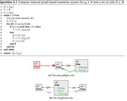
Algorithm 2.1Compute reduced graph-based transition system forq₀∈ G and a set of rulesR⊆ R.

1: Q:=

q0

2: T:=;

3: S:=

q0 4: whileS6=;do

5: Letqbe some element ofS 6: S:=S\q

7: for alls∈succ(q,R)do

8: if∃p∈Qsuch thats∼=pthen

9: T:=T∪

(q,p)

10: else

11: Q:=Q∪ {s}

12: T:=T∪

(q,s) 13: S:=S∪ {s}

14: end if 15: end for 16: end while

17: return

Q,T,q0

;

n2

Phil n1Fork

n0

Phil

−Waiting

+Eating has

has

right

(a)ThepickupRightrule.

n0

Phil

−Eating

+Done

+Thinking

n3

Fork

n2

Fork left

has

right

has

[image:15.595.94.514.72.407.2]

(b)ThedropForksrule.

Figure 2.4:Two graph transformation rules, used in Example 2.7.

implies that Linear Temporal Logic (LTL) or Computation Tree Logic (CTL) formulae that hold in one transition system also hold in an equivalent system (see, e.g.,[2]on bisimulation equivalence).

In Alg. 2.1 it is shown how a graph transition system modulo isomorphism can be derived from a start stateq₀and a set of rulesR. Thisisomorphism reductionis achieved by checking for isomorphism instead of checking for equality in line 8. For a set of state graphsS(initially containing only the initial stateq₀) the successor states are computed. If a successor state has been visited before, only a transition to that state is added (line 9), otherwise a new state is added to the set of statesQand toS and a transition to the new state is added to the set of transitions (lines 10–13).

Example 2.7. In Figure 2.4 there are two other graph transformation rules: pickupRight and

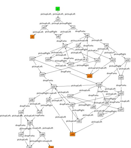
dropForks. ThepickupRightrule specifies that if a philosopher is in awaitingstate, meaning that he already has a left fork, he picks up the fork on his right if that fork is available. The philosopher changes toeatingstate. ThedropForksrule specifies that if a philosopher is in aneatingstate he may stop eating and drop the forks on his left and right hand side. The philosopher then changes tothinkingstate again and is markeddone, meaning that he already has had a meal. Thedoneflag can be used to check if every philosopher gets a meal, i.e., that the rule system does not result in starvation. Applying Algorithm 2.1 to the rulespickupLeft,pickupRight, anddropForksand the start state in Figure 2.1 results in a labelled transition system consisting of 40 states and 110 transitions, which is shown in Figure 2.5. Without isomorphism reduction the state space consists of 112 states and 314 transitions. The green node represents the start states0, which is the state in Figure 2.1, the orange nodes represent final states, i.e., states from which no transition is possible. This means that all philosophers are awaitingstate and none can get his right fork. Such a state is called adeadlock state. From the LTS it is clear that this rule system is not free of deadlocks. When one inspects the final states (not displayed here), it appears that the rule system is also not free of starvation, i.e., there are final states where not all philosophers have had a meal. Sometimes there are multiple labels on a single transitions, meaning that different transitions lead to an isomorphic state.

(16)

s0

s1

s2 s3

s4 s5 s6

s7 s8 s9

s10 _s11

s12 _s14 _s13 _s15

s16 s17 s18 s19 s20 s21 s22 s23 s24 s25 s26 s27 s28 s29 s30 s31 s32 s33 s34 s35 s36 s37 s38 s39

pickupLeft, pickupLeft, pickupLeft pickupLeft, pickupLeft, pickupLeft pickupLeft, pickupLeft, pickupLeft

pickupLeft, pickupLeft pickupLeft, pickupLeftpickupRight

pickupLeft pickupRight pickupLeft dropForks

dropForks pickupLeftpickupLeft pickupLeft

pickupLeft pickupLeft pickupRight pickupLeft pickupLeft pickupRight pickupLeft pickupLeft pickupRight pickupLeft pickupRight pickupLeft pickupRight dropForks pickupLeft pickupLeft pickupRight dropForks pickupLeft dropForks pickupLeft dropForks dropForks pickupLeft pickupLeft pickupLeft dropForks pickupLeft pickupLeft pickupRight _pickupLeft pickupLeft pickupRight pickupLeft pickupLeft pickupRight pickupLeft pickupRight pickupLeft pickupRight dropForks pickupLeft pickupLeft pickupRight dropForks pickupLeft dropForks pickupLeft dropForks dropForks pickupLeft, pickupLeft, pickupLeft pickupLeft, pickupLeft, pickupLeft pickupLeft, pickupLeft, pickupLeft

[image:16.595.92.551.130.648.2]

dropForks pickupLeft, pickupLeft pickupLeft, pickupLeft pickupRight pickupLeft pickupRight dropForks pickupLeft dropForks

(17)

2.4 Isomorphism and Isomorphism Reduction 11

Algorithm 2.2Compute the reduced graph-based transition system forq₀∈ G and a set of rules R⊆ Rusing a canonical representation functioncan.

1: r0:=can(q0)

2: Q:=

r0

3: T:=;

4: S:=

r0 5: whileS6=;do

6: Letqbe some element ofS 7: S:=S\q

8: for alls∈succ(q,R)do

9: r:=can(s)

10: ifr∈/Qthen 11: Q:=Q∪ {r}

12: S:=S∪ {r}

13: end if 14: T:=T∪

(q,r) 15: end for

16: end while

17: return

Q,T,q0

;

of successor states and communicate and store those canonical forms. The advantage of that being that isomorphism reduction is achieved independent of the way states are stored. For this we need a canonical representation function that is defined as follows:

Definition 2.8 (Canonical representation and canonical form). A canonical representation func-tioncan:G → G computes an isomorphism invariant graph representative for each graph that is isomorphic to that graph, i.e.,can(G)∼=Gfor allG∈ G, such that for every pair of graphsG,H∈ G,

can(G) =can(H)if and only ifG∼=H.

can(G)is called thecanonical formofG.

(18)

(19)

3

Architecture of Distributed Groove

In this chapter we describe the architecture that we use for distributed state space generation for graph transition systems. The task is distributed among severalworkers. Each worker may be a separate machine, but also multiple workers may run on the same machine. For the communication between the workersmessage passing(MPI) is used. Within the architecture a single worker consists roughly of four components.

GROOVE is used to compute successor states for state graphs, as described in Chapter 2.

LTSMIN is used for storing the state space and for facilitating the communication of states to and

from other workers.

BLISS is used for computing canonical forms forcoloured graphs. Coloured graphs are slightly different from the edge labelled graphs used in GROOVEand will be defined in Chapter 4. A conversion between edge labelled graphs and coloured graphs is used to compute canonical forms for edge labelled graphs (described in the same chapter).

Distributed GROOVE(DG) connects GROOVE, LTSMINand BLISSas described below. DG runs within

the same Java Virtual Machine (JVM) as GROOVEand uses Java method calls to communicate

with GROOVE.

JVM JVM

Groove Groove Groove

DG

LTSmin LTSmin

Bliss

DG

Bliss

DG

Bliss

LTSmin graphs

index vectors

index vectors coloured

graphs

MPI stdio

stdio

JVM

[image:19.595.133.465.516.657.2]

MPI MPI

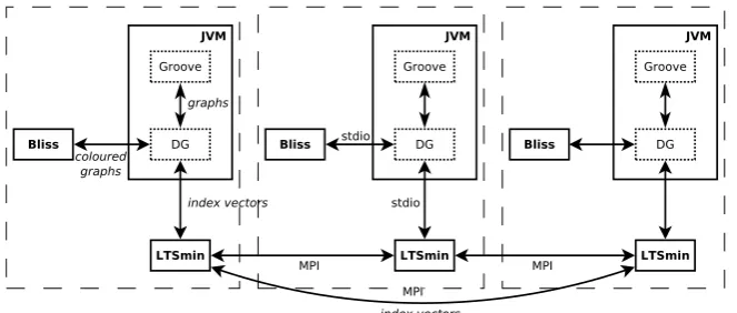
Figure 3.1:Schematic overview of the architecture.

How the tools relate to each other is depicted schematically in Figure 3.1. The workers are indicated by the dashed boxes. Each solid box in the figure represents a separate process, dotted boxes represent different tool instance within a JVM (for GROOVEand DG). The arrows represent

communication between the tool instances.

• DG communicates (synchronously) with BLISSusing pipes (standard input/output). Because

of this, currently DG and BLISSneed to run on the same machine. For each instance of DG a

(20)

14 Architecture of Distributed GROOVE

separate process of BLISSis run. DG sends a coloured graph to BLISSand receives its canonical

form back. Conversion of graphs is done on the side of DG.

• DG communicates (synchronously) with LTSMINusing either pipes (standard input/output)

or TCP/IP. For each instance of LTSMIN a separate process of DG is running. DG receives a state from LTSMIN, computes successor states using GROOVE, and sends canonical forms of the successor states back to LTSMIN. The state graphs are communicated between DG and LTSMIN

asstate vectors. This means that on receiving a state, DG needs to decode the state vector to a graph, and on sending successor states, the canonical forms have to be encoded as a state vector. Thisserialisationof graphs is described in Chapter 5. The state vectors are compressed intoindex vectors, i.e., both DG and LTSMINkeep a store of values used in the state vectors

and communicate a vector of indices of the values instead of a complete vector of values as representation of states. Of course, each new value has to be communicated once between DG and LTSMIN, so that they both know which index represents which value. This compression is

explained in Section 3.1.1.

• LTSMINtakes care of storing the labelled transition system, in which states are compressed even further usingtree compression, which is explained in Section 3.1.2. The different instances of LTSMINcommunicate with each other using MPI. LTSMINkeeps a global database of values used

and uses compressed index vectors for communication between workers. A hash function that is applied to index vectors is used to determine which worker is responsible for which state.

In the following sections we describe the functionality of LTSMIN(Section 3.1) and the functionality of DG and GROOVEin this distributed setting (Section 3.2).

3.1

LTS

MIN

The LTSMINtoolkit [23]contains sequential, symbolic, and distributed tools to generate labelled transition systems for various input languages, such as_µCRL, mCRL2, Promela (used in SPIN) and DVE (used in DiVinE). Bisimulation minimisation can be applied on the generated LTSs and several tools can be used to verify properties of the LTSs, such as CADP. LTSMINuses its own file format that

is optimised for efficient storage of LTSs and distributed writing to disc. States are represented as state vectors with a fixed length and compression of the state vectors is used for efficient storage and communication of states. The state vectors and index vector encoding are described in Section 3.1.1. A recursive compression technique calledtree compressionthat is used in LTSMINis described in

Section 3.1.2.

3.1.1

State vectors and index vectors

Definition 3.1(State vector). Astate vectoris a fixed-length vector of values~p=_p

0,p1, . . . ,pm

, i.e., a vector of which the lengthmis fixed. The values can be of arbitrary type and size.

The actual state vector is not communicated, but instead anindex vector, i.e., a vector containing the indexes of the values in a table.

LTSMIN uses a global store Pj for each of the parts of the vector.1 The complete so called

leaf databaseof values consists of the storesP₀,P₁, . . . ,Pm. Now the index vector of a state vector

p₀,p₁, . . . ,pm

is

i₀,i₁, . . . ,im

, whereijis the index of the valuepjin storePj.

This technique is used in, e.g., the SPIN model checker[14]and in LTSMIN[23]. It is based on the assumption that the number of different values of a certain part of the vector is relatively small with respect to the total number of different state vectors. For example, if multiple processes are modelled and local variables are stored in separate parts, then these parts are unchanged when an action of another processes is executed. Most changes are thenlocalto the process. If two parts are never changed by the same action or transition, they are calledindependent. The total number of states is of combinatorial nature, i.e., the total number of states that can be encoded is the product of the number of values of the different parts: |P₀| · |P₁| · · · |Pm|. The more locality there is in the state vectors,

the more space can be saved by storing the values of the parts separately and using an index vector,

1_{Actually, LTS}_MIN_{uses a store for each}_type_{(not further defined here), but the description here is accurate for how LTS}_MIN

(21)

3.1LTSMIN 15

containing the indexes of the values in the database as vector parts. The total number of values to be stored is not the product, but the sum of the number of values of the parts:|P₀|+|P₁|+· · ·+|Pm|.

Example 3.2. Letm=4 and let the leaf database contain the following values:

i P₀ P₁ P₂ P₃ 0 〈4, 5〉 7 “a” 49 1 〈1,2〉 1337 “b” 50 2 〈4, 2〉 0 “aa” 51 3 〈9, 5〉 50 “ab” 52 4 〈1, 1〉 2 “aba” 53

Now, value vector〈〈1, 2〉, 0, “aba”, 49〉is encoded as index vector〈1, 2, 4, 0〉.

For the examples we used (tuples of) integers and string for the values in the leaf database, but in LTSMINany serializable type of values may be used in the leaf database. The indexes are in the range

of natural numbers that can be encoded in 32 bits.

3.1.2

Tree Compression

These index vectors can also be partitioned into parts, which are then values for a next level of indexing. Parts of the index vector are stored again in a store, and the index of these parts in the store are used in the compressed vector. This is calledrecursive indexing[13]ortree compression[5].

Example 3.3. We explain the tree compression in LTSMIN by an example. For the index vector 〈1, 2, 4, 0〉from the previous example, tree compression is applied in the following way. First the vector is split into two parts:〈1, 2〉and〈4, 0〉. For the first part, the index is looked up in store I₀, for the second part in storeI₁:

i I₀ I₁ 0 〈0, 0〉 〈0, 0〉 1 〈1, 1〉 〈1, 1〉 2 〈1,2〉 〈2, 0〉 3 〈2, 0〉 〈3, 1〉 4 〈0, 1〉 〈4,0〉

Tuple〈1, 2〉has index 2 inI₀,〈4, 0〉has index 4 in storeI₁, so the vector〈〈1, 2〉, 0, “aba”, 49〉can be encoded as〈2, 4〉.

[image:21.595.227.369.134.207.2]

For larger vectors multiple levels of tree compression can be used. Theroottable consists of pairs of indexes representing states. Depending on the size of the state vectors, an index in a table of the tree compression datastructure points to either a value in the leaf database or to a value in a separate table one level lower. See[5]for an extensive description of tree compression in LTSMIN.

3.1.3

State compression and graphs

In the distributed setting we use canonical forms of state graphs to achieve isomorphism reduction. Canonically numbering nodes such as is done in NAUTY and BLISS renumbers the vertices of the

graph in a way that is difficult to predict and for which local changes (adding or removing one edge, renaming a label) may result in a completely different numbered graph. This means that when a straightforward serialisation of graphs is used, already a small change in the state graph may result in large changes in the state vector resulting from that state graph. Therefore it is not immediately clear if there will be any benefit in using the state compression of LTSMINfor graphs. Althought there will

perhaps be little locality of transitions, because of the renumbering of nodes, nonetheless the number of values per part may still be much less than the total number of states. It needs to be determined empirically if the state compression of LTSMINworks well for serialised graphs. The experiments in

(22)

16 Architecture of Distributed GROOVE

3.2

G

ROOVE

, DG, and the interface to LTS

MIN

The DG part of the distributed setup is responsible for computing successor states (using GROOVE), computing canonical forms (using BLISS), serialising graphs and compressing the resulting state vectors into index vectors. DG and GROOVEare started with agraph grammar, containing a set of

graph transformation rules, and astart graph, the graph representing the start state.

At initialisation, LTSMINstarts N LTSMINworkers andN instances of DG. Each instance of DG uses GROOVEas a library and loads the grammar and the start state that are to be explored. DG

communicates to LTSMINthe size of the state vectors used, which is either based on the number of

nodes in the start graph or on the number of different edge labels used in the system (depending on the particular serialisation used, see Chapter 5). DG computes a canonical form for the start graph using BLISSand sends a serialised form of the canonical start graph to LTSMIN.

The functionality of DG in this distributed setting is described in Algorithm 3.1. The following functions are used:

recvValues receives new values for the leaf database, i.e., values that have not been received before, and keeps a mapping between the values and their indexes in the leaf database;

recvIndexVector reads an index vector representing an open state, to be explored by the current worker;

decompress_V decompresses the index vector to a state vector using the mapping between indexes and values of the leaf database;

decode decodes state vectors to graphs (see Chapter 5);

succ computes successor state graphs for a given graph (see Chapter 2) and returns a list containing for each successor state graph ga tuple

l,g

containing a transition labell(which is the name of the transformation rule that resulted in the successor state) and the state graph g;

can computes a canonical form of a graph (see Chapter 4);

encode encodes a graph to a state vector (see Chapter 5);

compress_V andcompress_L compress state vectors and transition labels to index vectors and transi-tion label indexes respectively;

sendValues sends newly encountered part values and transition labels to LTSMIN;

(23)

3.2GROOVE,DG, and the interface toLTSMIN 17

Algorithm 3.1Functionality of DG in the distributed setting: receiving states from LTSMIN, computing

successor states and canonical forms, and communicating encoded successor states back to LTSMIN.

1: recvValues();

2: q_I:=recvIndexVector();

3: while(q_I6=null)do

4: q_V:=decompressV(qI); 5: g_q:=decode(q_V);

6: t:=l₁,g₁,l₂,g₂. . . ,lr,gr

:=succ(gq); 7: for1≤i≤rdo

8: c:=can(gi); 9: sV:=encode(c); 10: sI:=compressV(sV); 11: lI :=compressL(l);

12: sendValues();

13: sendTransition(lI,sI); 14: end for

15: recvValues();

16: q_I:=recvIndexVector();

(24)

(25)

4

Computing a Canonical Form

In the architecture of the distributed state space generation tool, described in the previous chapter, isomorphism reduction of the generated state space is achieved by computingcanonical formsof the state graphs, as defined in Definition 2.8. This chapter describes how to compute canonical forms of edge labelled graphs.1

Various tools exists that compute canonical form for coloured graphs, which is a slightly different graph formalism from the edge labelled graphs as defined in Chapter 2. Coloured graphs and other concepts used in this chapter will be defined in Section 4.1. In_[17_]an overview is provided of the tools that compute canonical forms of coloured graphs. In this report we use the tool BLISSby Junttila

& Kaski[15, 16], which is based on the tool NAUTYby McKay[20, 19]. In Section 4.2 we describe

the basic ideas and algorithms behind these tools. The reader that is not interested in the details of computing canonical forms may safely skip that section.

In order to be able to use the existing tools that use coloured graphs, a conversion is required from the edge-labelled graphs used in GROOVE to coloured graphs. The conversion that we use is presented in Section 4.3. A consequence of the conversion used, is that the size of the resulting graph is typically larger than the original graph. The size of the resulting graph is discussed in Section 4.3.2.

4.1

Definitions

We assume an ordered universe of vertex coloursC. In BLISSnatural numbers are used to represent

colours.

Definition 4.1(Coloured graph). Adirected graph Gis a tuple〈VG,EG〉with a finite nonempty set of

nodes(orvertices)VGand a set ofedges EG⊆VG×VG. The edges have associated source and target

functionssrc,tgt:EG →VG. A directed graphGis calledcolouredif it has an associated function

c:VG→C. The class of coloured graphs is denotedGC.

Definition 4.2(Isomorphism of coloured graphs). Let G=_〈V_G,E_G,c_G_〉and H =_〈V_H,E_H,c_H_〉be two coloured graphs. A bijective function f:V_G _→V_H is called anisomorphismif for all v_∈V_G cG(v) =cH(f(v))and for allv1,v2∈VG,

(v₁,v₂)_∈E_G _⇐⇒ (f(v₁),f(v₂))_∈E_H.

If such a function exists,GandHare calledisomorphic, denotedG∼₌H.

Definition 4.3(Permutation). Apermutationof a setAis a bijective function_α:A→A. The image of a∈Aunder a permutation_αis denoted_α₍a)oraα. The set of all permutations for a set{1, 2, . . . ,n} is denotedSn.

1_{This chapter is a compressed version of an earlier published technical report}_[₁₇_]_{. The technical report is partly written in}

the context of a research topics project and partly in the context of the final project, of which this report is the end product.

(26)

20 Computing a Canonical Form

A permutation can be represented as a matrix:

α=

1 2 · · · n 1α 2α · · · nα

∈S_n.

Definition 4.4(Graph permutation). Agraph permutationis a vertex permutationγ:V →V that associates with each directed coloured graphG=_〈V,E,c_〉a permuted graphGγ=_〈Vγ,Eγ,cγ_〉, where

Vγ=_{vγ_|v_∈V_}=V,

Eγ=_{(v₁γ,v₂γ)_|(v₁,v₂)_∈E_}, and cγ={(vγ,k)|(v,k)∈c}.

The set of all graph permutations for a set of verticesV is denotedSV.

For all permutationsγ∈SV it holds thatGγ∼=G. A special subset ofSV is the set ofautomorphisms

ofG, Aut(G) ={γ∈SV|Gγ=G}.

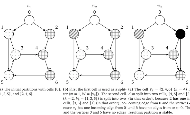
An important ingredient of the algorithm that will be described in the next section is partition refinement. Vertices of the graph are partitioned in equivalence classes. The initial partition of the vertices is based on the colours of the vertices. Then the partition is refined such that also the number of incoming and outgoing edges from the vertices is taken into account.

Definition 4.5(Partition). Apartitionπof a set of nodesV is a set{W₁,W₂, . . . ,W_r_}of nonempty disjointcells W_i_⊆V whose union isV. A partition with only trivial cells, i.e., cells that contain only one element, is called adiscrete partition. The partition that contains only one cell, the setV, is called theunit partition. The set of partitions ofV is denotedΠ(V). Anordered partitionofV is a sequence

(W₁,W₂, . . . ,Wr)such that the set{W1,W2, . . . ,Wr}is a partition ofV. The set of ordered partitions

ofV is denotedΠ e

(V).

The set of automorphisms for a graphGwith vertex partition_πis defined as Aut₍G,_π_{) =}{γ∈ SV|Gγ=G∧πγ=γ}.

In the following we denote the vertices as natural numbers, i.e., the set of verticesV is the set of numbers{1, 2, . . . ,n} ⊆Nwithn=|V|.

Definition 4.6(Partition permutation). Ifπ∈Π e

(V)is a discrete ordered partition, we define the permuted graph G(π), isomorphic toG, by relabelling the vertices ofGin the order that they appear inπ: givenπ= ({i₁},{i₂}, . . . ,{in})with{i1,i2, . . . ,in}={1, 2, . . . ,n}, the permuted graph, denoted

G(π), is defined as(G)δ, where the permutationδis given by

δ=

i₁ i₂ · · · in

1 2 · · · n

∈S_V.

This permutationδ, associated with partitionπ, is also written asπ. This partition permutation provides a relabelling of vertices based on a generated partition of vertices.

Example 4.7. As an example, suppose an isomorphismγ={17→2, 27→3, 37→1}that maps vertices of graphGto vertices ofH, with

V_G=V_H=_{1, 2, 3},

EG={(1,a, 2),(2,b, 3),(3,c, 1)}, and

E_H=_{(2,a, 3),(3,b, 1),(1,c, 2)}.

If we use some ordered partitionπ= ({i₁_},{i₂_},{i₃_})as a permutation ofG, then

(G)π= (H)πγ.

For instance, letπ= ({2},{1},{3}). Then

(EG)π={(2,a, 1),(1,b, 3),(3,c, 2)}, πγ= ({3},{2},{1}),

(EH)π γ

(27)

4.2 Computing a canonical form of vertex coloured graphs 21

Definition 4.8(Partition refinement). Given partitionsπ1,π2of some set,π1is called arefinement ofπ2orfinerthanπ2(andπ2is calledcoarserthanπ1), denotedπ1vπ2, if for all cellsVi∈π1

there exists a cellW_j_∈π2such thatV_i_⊆W_j.

The partition refinement algorithm used in computing the canonical form, to be described in Section 4.2 computes the coarsest stable refinement of a partition. Stability of a partition is based on the numbers of adjacent elements of the members of the cells of the partition.

Definition 4.9(Number of adjacent elements). Given a directed graphG=〈V,E〉and a partition

π∈Π(V), for an elementv_∈V and a cellW_∈π, the number of elements ofW which are adjacent inGtovis defined as:

d(v,W) =|

w∈W|(v,w)∈E∨(w,v)∈E | (4.1)

This definition considers edges in both directions. This differs from[20]where only one direction is used, which is related to the data structure used in NAUTY, which allows for easy comparison of

rows of the matrix, whereas comparing columns is more expensive. In the case of undirected graphs this does not make a difference, but for directed graphs it does.

Definition 4.10(Stable partition). A partitionπis calledstablefor a directed graphGif for every pair of cellsW_i,W_j_∈πthe number of adjacent elements inW_jis the same for each element inW_i, i.e., for all verticesv₁,v₂_∈W_iit holds thatd(v₁,W_j) =d(v₂,W_j). The set of all stable partitions of a setV is denotedΠS(V).

The stable partition resulting from the partition refinement algorithm is not necessarily a discrete partition, so the result of partition refinement can not immediately be used as permutation of the vertices. Each discrete partition is also stable, but fornvertices there aren! possible permutations and we want to find a unique partition that gives us a canonical relabelling. Therefore we need a search tree that we can search for candidate canonical permutations and we need a way to order the candidate permutations so that we can choose one. The generation of this search tree and the ordering of the permutations are discussed in Section 4.2.3 and 4.2.2.

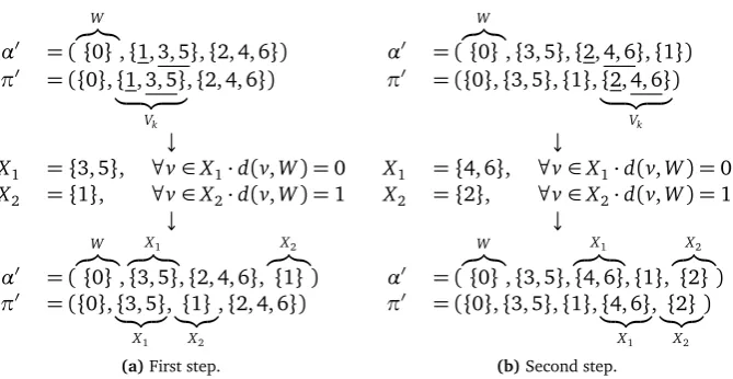
The partition refinement algorithm consists of iteratively splitting cells of the partition based on the number of adjacent elements of members of cells, until the partition is stable. The splitting of the cells of a partition_πis defined with respect to a setS(usually some cell of the partition) and denotedspl i t(π,S).

Definition 4.11(Split). For a partitionπ∈Π(V)and a setS⊆V, a partitionπ0=split(π,S)is a refinement of_πfor which for allW∈π, for allWi,Wj⊆WwithWi,Wj∈π0, it holds that

∀v₁∈Wi,v2∈Wj· d(v1,S) =d(v2,S) ⇐⇒ Wi=Wj

.

Ifsplit(π,S)=6 π,Sis called asplitterof_π.

4.2

Computing a canonical form of vertex coloured graphs

In this section it is explained how a canonical form of a directed coloured graph can be computed. McKay published an algorithm for finding a unique vertex labelling for isomorphic graphs[19], which is implemented in the tool NAUTY[20]. Improvements have been done by Junttila & Kaski in the tool

BLISS; the algorithm they describe is used in the remainder of this paper.

The idea is to generate for each graph a set of discrete partitions that can be used as permutation of the vertices of the graph, which results in a relabelled graph. If we have an ordering of the graphs, and if for isomorphic graphs the same set of relabelled graphs is generated, we can choose the minimum or maximum of the set as canonical form.

An easy but inefficient way of generating this set of graphs is generating all possible permutations of the vertices, which results in|V|! permutations of the set of verticesV. An ordering of the graphs can be obtained by representing each graph by a string that is a concatenation of the vertex colours and of the rows of the adjacency matrix (which represents the incident edges in the graph), and use an ordering on the strings.

The tools NAUTYand BLISSuse far more efficienct algorithms that do not generate all possible

(28)

1) A partition refinement algorithm that computes the unique coarsest stable partition for a given graph and initial partition of vertices;

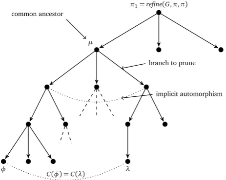
2) An algorithm that generates a search tree of stable partitions with discrete partitions as leaf nodes, of which one is chosen as the relabelling partition permutation leading to the canonical form.

The search tree is generated by first computing a stable partition (which is the root node of the tree) and then splitting one of the cells. For each of the members of the cell a subtree is added, where that member is put in a separate cell. Then each of the resulting partitions is stabilised again. This continues until all branches end in discrete partitions (the leaf nodes).

Because every intermediate partition is stabilised before it is split again, the number of nodes in the tree is reduced. The properties that are used in the partition refinement are isomorphism invariant, so the resulting set of permuted graphs stays equal for isomorphic graphs. This is required in order to be able to compute the canonical form.

In the next section the partition refinement algorithm is explained. In Sections 4.2.3 and 4.2.4 the generation and pruning of the search tree are described. An ordering of coloured graphs is given in Section 4.2.2.

4.2.1

Partition refinement algorithm

The vertices of a graph are partitioned into cells of vertices that are similar. Initially this partition is based on vertex colours, but this partition is refined based on the number of neighbours of vertices in other cells. The partition refinement algorithm and the result it produces are described in this section. The algorithm computes the unique coarsest stable refinement of a partition. The stability of partitions is defined in terms of numbers of adjacent vertices in the cells of the partition. A partition is stable if for each pair of elements of a cell the number of adjacent vertices is equal for both elements in all of the cells of the partitions (see Definition 4.10).

Suppose we have two isomorphic graphsG∼=H, withGα=H. Then ifπ1is a partition of vertices inGandπ2=πα₁ is a partition of vertices inH, equivalent toπ1, in the sense that(G)π1= (H)π2 (see Example 4.7). Then also the unique coarsest stable refinements ofπ1andπ2are equivalent. This is the case, because stability of partitions is defined such that it is isomorphism invariant, i.e., does not depend on the particular identities of vertices. It follows then from the uniqueness of the coarsest stable partition refinement and the isomorphism betweenGandH that the resulting stable partitions are equivalent (in the same sense of equivalence and by the same isomorphismα).

Unique coarsest stable refinement Here we prove that a unique coarsest stable refinement exists for each partition_π∈Π(V)of verticesV for a graphG. We assume that the setV is finite and hence also_Π(V), the set of all partitions ofV, is finite. We start with proving that the set of all partitions of a set forms a lattice (both a least upper bound and a greatest lower bound exists for each set of partitions). Then we prove that the least upper bound preserves stability. From the fact that each discrete partition is stable we can conlude that for each partition there exists a stable refinement (i.e. the discrete partition). It then follows that for each partition there exists a unique coarsest stable refinement.

Definition 4.12(Least upper bound of partitions). For a set of partitionsΠ⊆Π(V)and an ordering relationv, anupper boundis an elementπ∈Π(V)such that for all elementsρ∈Π,ρvπ. Theleast upper boundofΠ, denoted lubΠ, is the upper boundπsuch that for all other upper boundsρ,πvρ.

The least upper bound of a pair of elementsπ1,π2∈Π(V)is also calledjoin, denotedπ1tπ2. For computing this least upper bound we need the following relation.

Every partitionπ∈Π(V)can be considered as a binary equivalence relation where each pair reflects that two elements are in the same cell:

R=₍

s,t)∈V×V | ∃W∈π·s,t∈W (4.2)

(29)

4.2 Computing a canonical form of vertex coloured graphs 23

0

1

2

3

4

5

(a)Partitionπ1.

0

1

2

3

4

5

(b)Partitionπ2.

0

1

2

3

4

5

(c)The least upper bound ofπ1 andπ2,π1tπ2.

0

1

2 3

4 5

(d)RelationR1, reflecting the par-tition

{0, 1},{2, 3},{4, 5} .

0

1

2 3

4 5

(e)RelationR2, reflecting the par-tition

{0, 1},{2, 5},{3, 4} .

0

1

2 3

4 5

(f) The transitive closure of R1∪R2, reflecting the partition

{0, 1},{2, 3, 4, 5} .

Figure 4.1: The partitionsπ1andπ2, which are stable, and their least upper boundπ1tπ2. The partitions are shown by the colours of the vertices. The partitions can be seen as relations, where elements in the same cell are related. RelationR₁reflects partitions_π1,R₂reflects partition_π2, and the transitive closure ofR₁andR₂reflects the least upper boundπ1tπ2.

Proposition 4.13. Given a set of partitionsΠ =_{π1,π2, . . . ,πr} ⊆Π(V)and their associated binary

relations R₁,R₂, . . . ,R_r, the partitionπ0formed by the sets of vertices of maximal connected subgraphs of the union R₁_∪R₂_{∪ · · · ∪}R_r is the least upper bound ofΠ.

Now we show that the least upper bound of two stable partitions is itself stable as well.

Theorem 4.14. Given two stable partitionsπ1,π2∈ΠS(V), the least upper boundlub{π1,π2}is also

stable.

Proof. To prove: for allπ1,π2∈ΠS,π1tπ2∈ΠS.

1) First we observe that becauseπ1andπ2are refinements of their least upper bound, the cells of

π1tπ2are unions of cells inπ1and unions of cells inπ2.

2) Because the way the least upper bound is constructed there exists for each pair v,w ∈W, W∈π1tπ2a path

v=v₁,v₂, . . . ,vr=w

such that for all pairsv_i,v_i+₁(1≤i<r),∃W0_∈(π1_∪π2)_·v_i,v_i+₁_∈W0.

3) Becauseπ1andπ2are stable, each pairvi,vi+1has the same number of neighbouring elements

for all cells of either_π1or_π2, so certainly for unions of cells in_π1or of cells in_π2.

4) Hence, by induction onr, the same holds for the pairv,w. So,π1tπ2must also be stable.

Definition 4.15(Greatest lower bound of partitions). Given a set of partitionsΠ⊆Π(V)and an ordering relationv, alower boundis an elementπ∈Π(V)such that for all elementsρ∈Π,πvρ. Thegreatest lower boundofΠ, denoted glbΠ, is the upper boundπsuch that for all other lower boundsρ,ρvπ.