Selectional Preferences for Semantic Role Classification

Semantic Role Classification

Be ˜nat Zapirain

University of the Basque Country

Eneko Agirre

University of the Basque Country

Llu´ıs M`arquez

Universitat Polit`ecnica de Catalunya

Mihai Surdeanu

This paper focuses on a well-known open issue in Semantic Role Classification (SRC) research: the limited influence and sparseness of lexical features. We mitigate this problem using models that integrate automatically learned selectional preferences (SP). We explore a range of models based on WordNet and distributional-similarity SPs. Furthermore, we demonstrate that the SRC task is better modeled by SP models centered on both verbs and prepositions, rather than verbs alone. Our experiments with SP-based models in isolation indicate that they outperform a lexical baseline with 20 F1 points in domain and almost 40 F1points out of domain. Furthermore, we show that a state-of-the-art SRC system extended with features based on selectional preferences performs significantly better, both in domain (17% error reduction) and out of domain (13% error reduction). Finally, we show that in an end-to-end semantic role labeling system we obtain small but statistically significant improvements, even though our modified SRC model affects only approximately 4% of the argument candidates. Our post hoc error analysis indicates that the SP-based features help mostly in situations where syntactic information is either incorrect or insufficient to disambiguate the correct role.

∗Informatika Fakultatea, Manuel Lardizabal 1, 20018 Donostia, Basque Country. E-mail:[email protected].

∗∗Informatika Fakultatea, Manuel Lardizabal 1, 20018 Donostia, Basque Country. E-mail:[email protected].

†UPC Campus Nord (Omega building), Jordi Girona 1–3, 08034 Barcelona, Catalonia. E-mail:[email protected].

‡1040 E. 4th Street, Tucson, AZ 85721. E-mail:[email protected].

Submission received: 14 November 2011; revised submission received: 31 May 2012; accepted for publication: 15 August 2012.

1. Introduction

Semantic Role Labeling (SRL) is the problem of analyzing clause predicates in text by identifying arguments and tagging them with semantic labels indicating the role they play with respect to the predicate. Such sentence-level semantic analysis allows the determination of who did what to whom, when and where, and thus characterizes the participants and properties of the events established by the predicates. For instance, consider the following sentence, in which the arguments of the predicateto sendhave been annotated with their respective semantic roles.1

(1) [Mr. Smith]Agentsent[the report]Object[to me]Recipient[this morning]Temporal.

Recognizing these event structures has been shown to be important for a broad spectrum of NLP applications. Information extraction, summarization, question answering, machine translation, among others, can benefit from this shallow semantic analysis at sentence level, which opens the door for exploiting the semantic relations among arguments (Boas 2002; Surdeanu et al. 2003; Narayanan and Harabagiu 2004; Melli et al. 2005; Moschitti et al. 2007; Higashinaka and Isozaki 2008; Surdeanu, Ciaramita, and Zaragoza 2011). In M`arquez et al. (2008) the reader can find a broad introduction to SRL, covering several historical and definitional aspects of the problem, including also references to the main resources and systems.

State-of-the-art systems leverage existing hand-tagged corpora (Fillmore, Ruppenhofer, and Baker 2004; Palmer, Gildea, and Kingsbury 2005) to learn supervised machine learning systems, and typically perform SRL in two sequential steps: argument identification and argument classification. Whereas the former is mostly a syntactic recognition task, the latter usually requires semantic knowledge to be taken into account. The semantic knowledge that most current systems capture from text is basically limited to the predicates and the lexical units contained in their arguments, including the argument head. These “lexical features” tend to be sparse, especially when the training corpus is small, and thus SRL systems are prone to overfit the training data and generalize poorly to new corpora (Pradhan, Ward, and Martin 2008). As a simplified example of the effect of sparsity, consider the following sentences occurring in an imaginary training data set for SRL:

(2) [JFK]Patientwas assassinated[in Dallas]Location

(3) [John Lennon]Patientwas assassinated[in New York]Location

(4) [JFK]Patientwas assassinated[in November]Temporal

(5) [John Lennon]Patientwas assassinated[in winter]Temporal

All four sentences share the same syntactic structure, so the lexical features (i.e., the wordsDallas,New York,November, andwinter) represent the most relevant knowledge for discriminating between the Location and Temporal adjunct labels in learning.

1 For simplicity, in this paper we talk about arguments in the most general sense. Unless noted otherwise,

The problem is that, as in the following sentences, for the same predicate, one may encounter similar expressions with new words like Texas or December, which the classifiers cannot match with the lexical features seen during training, and thus become useless for classification:

(6) [Smith]was assassinated[in Texas]

(7) [Smith]was assassinated[in December]

This problem is exacerbated when SRL systems are applied to texts coming from new domains where the number of new predicates and argument heads increases considerably. The CoNLL-2004 and 2005 evaluation exercises on semantic role labeling (Carreras and M`arquez 2004, 2005) reported a significant performance degradation of around 10 F1 points when applied to out-of-domain texts from the Brown corpus.

Pradhan, Ward, and Martin (2008) showed that this performance degradation is essentially caused by the argument classification subtask, and suggested the lexical data sparseness as one of the main reasons.

In this work, we will focus on Semantic Role Classification (SRC), and we will show that selectional preferences (SP) are useful for generalizing lexical features, helping fight sparseness and domain shifts, and improving SRC results. Selectional preferences try to model the kind of words that can fill a specific argument of a predicate, and have been widely used in computational linguistics since the early days (Wilks 1975). Both semantic classes from existing lexical resources like WordNet (Resnik 1993b) and distributional similarity based on corpora (Pantel and Lin 2000) have been successfully used for acquiring selectional preferences, and in this work we have used several of those models.

The contributions of this work to the field of SRL are the following:

1. We formalize and implement a method that applies several selectional preference models to Semantic Role Classification, introducing for the first time the use of selectional preferences for prepositions, in addition to selectional preferences for verbs.

2. We show that the selectional preference models are able to generalize lexical features and improve role classification performance in a controlled experiment disconnected from a complete SRL system. The positive effect is consistently observed in all variants of WordNet and distributional similarity measures and is especially relevant for out-of-domain data. The separate learning of SPs for verbs and prepositions contributes

significantly to the improvement of the results.

3. We integrate the information of several SP models in a state-of-the-art SRL system (SwiRL)2_{and obtain significant improvements in semantic role}

classification and, as a consequence, in the end-to-end SRL task. The key for the improvement lies in the combination of the predictions provided bySwiRLand the several role classification models based on selectional preferences.

4. We present a manual analysis of the output of the combined role

classification system. By observing a set of real examples, we categorized and quantified the situations in which SP models tend to help role classification. By inspecting also a set of negative cases, this analysis also sheds light on the limitations of the current approach and identifies opportunities for further improvements.

The use of selectional preferences for improving role classification was first pre-sented in Zapirain, Agirre, and M`arquez (2009), and later extended in Zapirain et al. (2010) to a full-fledged SRC system. In the current paper, we provide more detailed background information and details of the selectional preference models, as well as complementary experiments on the integration in a full-fledged system. More impor-tantly, we incorporate a detailed analysis of the output of the system, comparing it with that of a state-of-the-art SRC system not using SPs.

The rest of the paper is organized as follows. Section 2 provides background on the automatic acquisition of selectional preference, and its recent relation to the semantic role labeling problem. In Section 3, the SP models investigated in this paper are ex-plained in all their variants. The results of the SP models in laboratory conditions are presented in Section 4. Section 5 describes the method for integrating the SP models in a state-of-the-art SRL system and discusses the results obtained. In Section 6 the qualita-tive analysis of the system output is presented, including a detailed discussion of several examples. Finally, Section 7 concludes and outlines some directions for future research.

2. Background

The simplest model for generating selectional preferences would be to collect all heads filling each role of the target predicate. This is akin to the lexical features used by current SRL systems, and we refer to this model as the lexical model. More concretely, the lexical model forverb-roleselectional preferences consists of the list of words appearing as heads of the role arguments of the predicate verb. This model can be extracted automatically from the SRL training corpus using straightforward techniques. When using this model for role classification, it suffices to check whether the head word of the argument matches any of the words in the lexical model. The lexical model is the baseline for our other SP models, all of which build on that model.

In order to generalize the lexical model, semantic classes can be used. Although in principle any lexical resource listing semantic classes for nouns could be applied, most of the literature has focused on the use of WordNet (Resnik 1993b). In the WordNet-based model, the words occurring in the lexical model are projected over the semantic hierarchy of WordNet, and the semantic classes which represent best those words are selected. Given a new example, the SRC system has to check whether the new word matches any of those semantic classes. For instance, in example sentences (2)–(5), the semantic class<time period>covers both training examples forTemporal(i.e.,November

and winter), and <geographical area> covers the examples forLocation. When test wordsTexasandDecemberoccur in Examples (6) and (7), the semantic classes to which they belong can be used to tag the first asLocationand the second asTemporal.

but, in order to speed up its use, it has also been used to produce off-line a full thesauri, storing, for every word, the weighted list of all outstanding similar words (Lin 1998). In theDistributional similarity model, when test itemTexas in Example (6) is to be labeled, the higher similarity toDallasandNew York, in contrast to the lower similarity toNovemberandwinter, would be used to label the argument with theLocationrole.

The automatic acquisition of selectional preferences is a well-studied topic in NLP. Many methods using semantic classes and selectional preferences have been proposed and applied to a variety of syntactic–semantic ambiguity problems, including syntactic parsing (Hindle 1990; Resnik 1993b; Pantel and Lin 2000; Agirre, Baldwin, and Martinez 2008; Koo, Carreras, and Collins 2008; Agirre et al. 2011), word sense disambiguation (Resnik 1993a; Agirre and Martinez 2001; McCarthy and Carroll 2003), pronoun res-olution (Bergsma, Lin, and Goebel 2008) and named-entity recognition (Ratinov and Roth 2009). In addition, selectional preferences have been shown to be effective to improve the quality of inference and information extraction rules (Pantel et al. 2007; Ritter, Mausam, and Etzioni 2010). In some cases, the aforementioned papers do not mention selectional preferences, but all of them use some notion of preferring certain semantic types over others in order to accomplish their respective task.

In fact, one could use different notions of semantic types. In one extreme, we would have a small set of coarse semantic classes. For instance, some authors have used the 26 so-called “semantic fields” used to classify all nouns in WordNet (Agirre, Baldwin, and Martinez 2008; Agirre et al. 2011). The classification could be more fine-grained, as defined by the WordNet hierarchy (Resnik 1993b; Agirre and Martinez 2001; McCarthy and Carroll 2003), and other lexical resources could be used as well. Other authors have used automatically induced hierarchical word classes, clustered according to occurrence information from corpora (Koo, Carreras, and Collins 2008; Ratinov and Roth 2009). On the other extreme, each word would be its own semantic class, as in the lexical model, but one could also model selectional preference using distributional similarity (Grefenstette 1992; Lin 1998; Pantel and Lin 2000; Erk 2007; Bergsma, Lin, and Goebel 2008). In this paper we will focus on WordNet-based models that use the whole hierarchy and on distributional similarity models, and we will use the lexical model as baseline.

2.1 WordNet-Based Models

Resnik (1993b) proposed the modeling of selectional preferences using semantic classes from WordNet and applied the model to tackle some ambiguity issues in syntax, such as noun-compounds, coordination, and prepositional phrase attachment. Given two alternative structures, Resnik used selectional preferences to choose the attachment maximizing the fitness of the head to the selectional preferences of the attachment points. This is similar to our task, but in our case we compare the target head to the selec-tional preference models for each possible role label (i.e., given a verb and the head of an argument, we need to find the role with the selectional preference that fits the head best). In Resnik’s model, he first characterizes the restrictiveness of the selectional pref-erence of an argument positionrof a governing predicatep, noted asR(p,r). For that, given a set of classesCfrom the WordNet nominal hierarchies, he takes the relative en-tropy or Kullback-Leibler distance between the prior distributionP(C) and the posterior distributionP(C|p,r):

R(p,r)=

c∈C

P(c|p,r)logP(c|p,r)

The priors can be computed from any corpora, computing frequencies of classes and using maximum likelihood estimates. The frequencies for classes cannot be directly observed, but they can be estimated from the lexical frequencies of the nouns under the class, as in Equation (2). Note that in WordNet, hypernyms (“hyp” for short) correspond to superclass relations, and therefore hyp(n) returns all superclasses of nounn.

freq(c)=

{n|c∈hyp(n)}

freq(n) (2)

A complication arises because of the polysemy of nouns. If each occurrence of a noun counted once in all classes that its senses belong to, polysemous nouns would account for more probability mass than monosemous nouns, even if they occurred the same number of times. As a solution, the frequency of polysemous nouns is split among its senses uniformly. For instance, the probability of the class <time period>can be estimated according to the frequencies of nouns like November,spring, and the rest of nouns under it.Novemberhas a single sense, so every occurrence counts as 1, butspring

has six different senses, so each occurrence should only count as 0.16. Note that with this method we are implicitly dealing with the word sense ambiguity problem. When encountering a polysemous noun as an argument of a verb, we record the occurrence of all of its senses. Given enough occurrences of nouns, the classes generalizing the intended sense of the nouns will gather more counts than competing classes. In the example,<time period>would have 1.16 compared with 0.16<tool>(i.e., for the metal elastic device meaning ofspring). Researchers have used this fact to perform Word Sense Disambiguation using selectional preferences (Resnik 1993a; Agirre and Martinez 2001; McCarthy and Carroll 2003).

The posterior probability can be computed similarly, but it takes into account occur-rences of the nouns in the required argument position of the predicate, and thus requires a corpus annotated with roles.

The selectional preference of a predicatepand rolerfor a headw0 of any potential argument, noted asSPRes(p,r,w0), is formulated as follows:3

SPRes(p,r,w0)= max

c0∈hyp(w0)

P(c0|p,r)logP(c0|p,r) P(c0)

R(p,r) (3)

The numerator formalizes the goodness of fit for the best semantic class c0 that

contains w0. The hypernym (i.e., superclass) of w0 yielding the maximum value is

chosen. The denominator models how restrictive the selectional preference is forpand

r, as modeled in Equation (1).

Variations of Resnik’s idea to find a suitable level of generalization have been explored in later years. Li and Abe (1998) applied the minimum-description length principle. Alternatively, Clark and Weir (2002) devised a procedure to decide when a class should be preferred rather than its children.

Brockmann and Lapata (2003) compared several class-based models (including Resnik’s selectional preferences) on a syntactic plausibility judgment task for German.

The models return weights for (verb, syntactic function, noun) triples, and correla-tion with human plausibility judgment is used for evaluacorrela-tion. Resnik’s seleccorrela-tional preference scored best among WordNet-based methods (Li and Abe 1998; Clark and Weir 2002). Despite its earlier publication, Resnik’s method is still the most popular representative among WordNet-based methods (Pad ´o, Pad ´o, and Erk 2007; Erk, Pad ´o, and Pad ´o 2010; Baroni and Lenci 2010). We also chose to use Resnik’s model in this paper.

One of the disadvantages of the WordNet-based models, compared with the distri-butional similarity models, is that they require that the heads are present in WordNet. This limitation can negatively influence the coverage of the model, and also its general-ization ability.

2.2 Distributional Similarity Models

Distributional similaritymodels assume that a word is characterized by the words it co-occurs with. In the simplest model, co-occurring words are taken from a fixed-size context window. Each wordwwould be represented by the set of words that co-occur with it,T(w). In a more elaborate model, each wordwwould be represented as a vector of wordsT(w) with weights, whereTi(w) corresponds to the weight of theith word in the vector. The weights can be calculated following a simple frequency of co-occurrence, or using some other formula.

Then, given two wordswandw0, their similarity can be computed using any

simi-larity measure between their co-occurrence sets or vectors. For instance, early work by Grefenstette (1992) used the Jaccard similarity coefficient of the two setsT(w) andT(w0)

(cf. Equation (4) in Figure 1). Lee (1999) reviews a wide range of similarity functions, including Jaccard and the cosine between two vectorsT(w) andT(w0) (cf. Equation (5)

in Figure 1).

In the context of lexical semantics, the similarity measure defined by Lin (1998) has been very successful. This measure (cf. Equation (6) in Figure 1) takes into account syntactic dependencies (d) in its co-occurrence model. In this case, the setT(w) of co-occurrences ofwcontains pairs (d,v) of dependencies and words, representing the fact

simJac(w,w0)= |

T(w)∩T(w0)|

|T(w)∪T(w0)|

(4)

simcos(w,w0)=

n

i=1Ti(w)Ti(w0)

n

i=1Ti(w)2

n

i=1Ti(w0)2

(5)

simLin(w,w0)=

(d,v)∈T(w)∩T(w0)(I(w,d,v)+I(w0,d,v))

(d,v)∈T(w)I(w,d,v)+

(d,v)∈T(w0)I(w0,d,v)

(6)

Figure 1

Similarity measures used in the paper.Jacandcosstand for Jaccard and cosine similarity metrics. T(w) is the set of words co-occurring withw,Ti(w) is the weight of theith element of the vector

that the corpus contains an occurrence ofwhaving dependencydwithv. For instance, if the corpus containsJohn loves Mary, then the pair(ncsubj, love)would be in the set

TforJohn. The measure uses information-theoretic principles, andI(w,d,v) represents the information content of the triple (Lin 1998).

Although the use of co-occurrence vectors for words to compute similarity has been standard practice, some authors have argued for more complex uses. Sch ¨utze (1998) builds vectors for each context of occurrence of a word, combining the co-occurrence vectors for each word in the context. The vectors for contexts were used to induce senses and to improve information retrieval results. Edmonds (1997) built a lexical co-occurrence network, and applied it to a lexical choice task. Chakraborti et al. (2007) used transitivity over co-occurrence relations, with good results on several classification tasks. Note that all these works usesecond orderandhigher orderto refer to their method. In this paper, we will also usesecond orderto refer to a new method which goes beyond the usual co-occurrence vectors (cf. Section 3.3).

A full review of distributional models is out of the scope of this paper, as we are in-terested in showing that some of those models can be used successfully to improve SRC. Pad ´o and Lapata (2007) present a review of distributional models for word similarity, and a study of several parameters that define a broad family of distributional similarity models, including Jaccard and Lin. They provide publicly available software,4 which we have used in this paper, as explained in the next section. Baroni and Lenci (2010) present a framework for extracting distributional information from corpora that can be used to build models for different tasks.

Distributional similarity models were first used to tackle syntactic ambiguity. For instance, Pantel and Lin (2000) obtained very good results on PP-attachment using the distributional similarity measure defined by Lin (1998). Distributional similarity was used to overcome sparsity problems: Alongside the counts in the training data of the target words, the counts of words similar to the target ones were also used. Although not made explicit, Lin was actually using a distributional similarity model of selectional preferences.

The application of distributional selectional preferences to semantic roles (as op-posed to syntactic functions) is more recent. Gildea and Jurafsky (2002) are the only ones applying selectional preferences in a real SRL task. They used distributional clustering and WordNet-based techniques on a SRL task on FrameNet roles. They report a very small improvement of the overall performance when using distributional clustering techniques. In this paper we present complementary experiments, with a different role set and annotated corpus (PropBank), a wider range of selectional preference models, and the analysis of out-of-domain results.

Other papers applying semantic preferences in the context of semantic roles rely on the evaluation of artificial tasks or human plausibility judgments. Erk (2007) introduced a distributional similarity–based model for selectional preferences, reminiscent of that of Pantel and Lin (2000). Her approach models the selectional preferenceSPsim(p,r,w0)

of an argument position r of governing predicate p for a possible head-word w0 as

follows:

SPsim(p,r,w0)=

w∈Seen(p,r)

sim(w0,w)·weight(p,r,w) (7)

wheresim(w0,w) is the similarity between the seen and potential heads,Seen(p,r) is the set of heads of rolerfor predicatepseen in the training data set (as in the lexical model), andweight(p,r,w) is the weight of the seen head wordw. Our distributional model for selectional preferences follows her formalization.

Erk instantiated the basic model with several corpus-based distributional similarity measures, including Lin’s similarity, Jaccard, and cosine (Figure 1) among others, and several implementations of the weight function such as the frequency. The quality of each model instantiation, alongside Resnik’s model and an expectation maximization (EM)-based clustering model, was tested in a pseudo-disambiguation task where the goal was to distinguish an attested filler of the role and a randomly chosen word. The results over 100 frame-specific roles showed that distributional similarities attain similar error rates to Resnik’s model but better than EM-based clustering, with Lin’s formula having the smallest error rate. Moreover, the coverage of distributional similarity mea-sures was much better than Resnik’s. In a more recent paper, Erk, Pad ´o, and Pad ´o (2010) extend the aforementioned work, including evaluation to human plausibility judgments and a model for inverse selectional preferences.

In this paper we test similar techniques to those presented here, but we evaluate selectional preference models in a setting directly related to semantic role classification, namely, given a selectional preference model for a verb we find the role which fits best the given head word. The problem is indeed qualitatively different from previous work in that we do not have to choose among the head words competing for a role but among selectional preferences of roles competing for a head word.

More recent work on distributional selectional preference has explored the use of discriminative models (Bergsma, Lin, and Goebel 2008) and topical models ( ´O S´eaghdha 2010; Ritter, Mausam, and Etzioni 2010). These models would be a nice addition to those implemented in this paper, and if effective, they would improve further our results with respect to the baselines which don’t use selectional preferences.

Contrary to WordNet-based models, distributional preferences do not rely on a hand-built resource. Their coverage and generalization ability depend on the corpus from which the distributional similarity model was computed. This fact makes this approach more versatile in domain adaptation scenarios, as more specific and test-set focused generalization corpora could be used to modify, enrich, or even replace the original corpus.

2.3 PropBank

In this work we use the semantic roles defined in PropBank. The Proposition Bank (Palmer, Gildea, and Kingsbury 2005) emerged as a primary resource for research in SRL. It provides semantic role annotation for all verbs in the Penn Treebank corpus. PropBank takes a “theory-neutral” approach to the designation of core semantic roles. Each verb has a frameset listing its allowed role labelings in which the arguments are designated by number (starting from 0). Each numbered argument is provided with an English language description specific to that verb. The most frequent roles are Arg0 and Arg1 and, generally, Arg0 stands for the prototypical agent and Arg1 corresponds to the prototypical patient or theme of the proposition. The rest of arguments (Arg2 to Arg5) do not generalize across verbs, that is, they have verb specific interpretations.

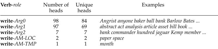
Table 1

Example ofverb-rolelexical SP models forwrite, listed in alphabetical order. Number of heads indicates the number of head words attested, Unique heads indicates the number of distinct head words attested, and Examples lists some of the heads in alphabetical order.

Verb-role Number of Unique Examples

heads heads

write-Arg0 98 84 Angrist anyone baker ball bank Barlow Bates ...

write-Arg1 97 69 abstract act analysis article asset bill book ...

write-Arg2 7 7 bank commander hundred jaguar Kemp member ...

write-AM-LOC 2 2 paper space

write-AM-TMP 1 1 month

(modal verb), AM-NEG (negation marker), AM-PNC (purpose), AM-PRD (predication), AM-REC (reciprocal), and AM-TMP (temporal).

3. Selectional Preference Models for Argument Classification

Our approach for applying selectional preferences to semantic role classification is discriminative. That is, the SP-based models provide a score for every possible role label given a verb (or preposition), the head word of the argument, and the selectional preferences for the verb (or preposition). These scores can be used to directly assign the most probable role or to codify new features to train enriched semantic role classifiers.

In this section we first present all the variants for acquiring selectional preferences used in our study, and then present the method to apply them to semantic role classifi-cation. We selected several variants that have been successful in some previous works.

3.1 Lexical SP Model

In order to implement the lexical model we gathered all headswof arguments filling a rolerof a predicatepand obtainedfreq(p,r,w) from the corresponding training data (cf. Section 4.1). Table 1 shows a sample of the heads of arguments attested in the corpus for the verbwrite. The lexical SP model can be simply formalized as follows:

SPlex(p,r,w0)=freq(p,r,w0) (8)

3.2 WordNet-Based SP Models

We instantiated the model based on (Resnik 1993b) presented in the previous sec-tion (SPRes, cf. Equation (3)) using the implementation of Agirre and Martinez (2001). Tables 2 and 3 show the synsets5 _{that generalize best the head words in Table 1}

for write-Arg0and write-Arg1, according to the weight assigned to those synsets by Equation (1). According to this model, and following basic intuition, the words attested as being Arg0s ofwriteare best generalized by semantic classes such as living things,

Table 2

Excerpt from the selectional preferences forwrite-Arg0according toSPRes, showing the synsets

that generalize best the head words in Table 1. Weight lists the weight assigned to those synsets by Equation (1). Description includes the words and glosses in the synset.

Synset Weight Description

n#00002086 5.875 life form organism being living thingany living entity n#00001740 5.737 entity somethinganything having existence(living or nonliving) n#00009457 4.782 object physical objecta physical (tangible and visible) entity; n#00004123 4.351 person individual someone somebody mortal human soul

a human being;

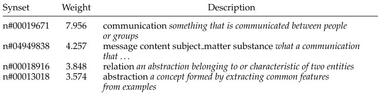
Table 3

Excerpt from the selectional preferences forwrite-Arg1according toSPRes, showing the synsets

that generalize best the head words in Table 1. Weight lists the weight assigned to those synsets by Equation (1). Description includes the words and glosses in the synset.

Synset Weight Description

n#00019671 7.956 communicationsomething that is communicated between people or groups

n#04949838 4.257 message content subject matter substancewhat a communication that . . .

n#00018916 3.848 relationan abstraction belonging to or characteristic of two entities n#00013018 3.574 abstractiona concept formed by extracting common features

from examples

entities, physical objects, and human beings, whereas Arg1s by communication, mes-sage, relation, and abstraction.

Resnik’s method performs well among Wordnet-based methods, but we realized that it tends to overgeneralize. For instance, in Table 2, the concept for “entity” (one of the unique beginners of the WordNet hierarchy) has a high weight. This means that a head like “grant” would be assigned Arg0. In fact, any noun which is under concept n#00001740 (entity) but not under n#04949838 (message) would be assigned Arg0. This observation led us to speculate on an alternative method which would try to generalize as little as possible.

Our intuition is that general synsets can fit several selectional preferences at the same time. For instance, the<entity>class, as a superclass of most words, would be a correct generalization for the selectional preferences of allagent,patient, andinstrument

roles of a predicate likebreak. On the contrary, specific concepts are usually more useful for characterizing selectional preferences, as in the<tool>class for theinstrumentrole ofbreak. The priority of using specific synsets over more general ones is, thus, justified in the sense that they may better represent the most relevant semantic characteristics of the selectional preferences.

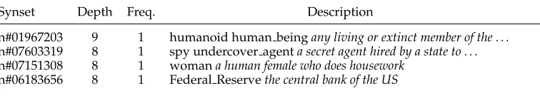
Table 4

Excerpt from the selectional preferences forwrite-Arg0according toSPwn, showing from deeper

to shallower the synsets in WordNet which are connected to head words in Table 1. Depth lists the depth of synsets in WordNet. Description includes the words and glosses in the synset.

Synset Depth Freq. Description

n#01967203 9 1 humanoid human beingany living or extinct member of the . . . n#07603319 8 1 spy undercover agenta secret agent hired by a state to . . . n#07151308 8 1 womana human female who does housework

n#06183656 8 1 Federal Reservethe central bank of the US

Table 5

Excerpt from the selectional preferences forwrite-Arg1according toSPwn, showing from deeper

to shallower the synsets in WordNet which are connected to head words in Table 1. Depth lists the depth of synsets in WordNet. Description includes the words and glosses in the synset.

Synset Depth Freq. Description

n#05403815 13 1 informationformal accusation of a crime

n#05401516 12 1 accusation accusala formal charge of wrongdoing brought . . . n#04925620 11 1 charge complainta pleading describing some wrong or offense n#04891230 11 1 memoiran account of the author’s personal experiences

More concretely, we model selectional preferences as a multiset6of synsets, storing all hypernyms of the heads seen in the training data for a certain role of a given predicate, that is:

Smul(p,r)=

w∈Seen(p,r)

hyp(w) (9)

whereSeen(p,r) are all the argument heads for predicatepand roler, andhyp(w) returns all the synsets and hypernyms ofw, including hypernyms of hypernyms recursively up to the top synsets.

For any given synsets, letd(s) be the depth of the synset in the WordNet hierarchy, and let1Smul(p,r)(s) be the multiplicity function which returns how many timessis con-tained in the multisetSmul(p,r). We define a partial order among synsetsa,b∈Smul(p,r) as follows: ord(a)>ord(b) iff d(a)>d(b) or d(a)=d(b)∧1Smul(p,r)(a)>1Smul(p,r)(b). Tables 4 and 5 show the most specific synsets (according to their depth) forwrite-Arg0

andwrite-Arg1.

We can then measure the goodness of fit of the selectional preference for a word as the rank in the partial order of the first hypernym of the head that is also present in the selectional preference. For that, we introduceSPwn(p,r,w), which following the previous notation is defined as:

SPwn(p,r,w)=arg max s∈hyp(w)∩Smul(p,r)

ord(s) (10)

Table 6

Most similar words forTexasandDecemberaccording to Lin (1998).

Texas Florida 0.249, Arizona 0.236, California 0.231, Georgia 0.221, Kansas 0.217, Minnesota 0.214, Missouri 0.214, Michigan 0.213, Colorado 0.208, North Carolina 0.207, Oklahoma 0.207, Arkansas 0.205, Alabama 0.205, Nebraska 0.201, Tennessee 0.197, New Jersey 0.194, Illinois 0.189, Virginia 0.188, Kentucky 0.188, Wisconsin 0.188, Massachusetts 0.184, New York 0.183

December June 0.341, October 0.340, November 0.333, April 0.330, February 0.329, September 0.328, July 0.323, January 0.322, August 0.317, may 0.305, March 0.250, Spring 0.147, first quarter 0.135, mid-December 0.131, month 0.130, second quarter 0.129, mid-November 0.128, fall 0.125, summer 0.125, mid-October 0.121, autumn 0.121, year 0.121, third quarter 0.119

In case of ties, the role coming first in alphabetical order would be returned. Note that, similar to the Resnik model (cf. Section 2.1), this model implicitly deals with the word ambiguity problem.

As with any other approximation to measure specificity of concepts, the use of depth has some issues, as some deeply rooted stray synsets would take priority. For instance, Table 4 shows that synset n#01967203 forhuman beingis the deepest synset. In practice, when we search the synsets of a target word in theSPwnmodels following Eq. (10), the most specific synsets (specially stray synsets) are not found, and synsets higher in the hierarchy are used.

3.3 Distributional SP Models

All our distributional SP models are based on Equation (7). We have used several vari-ants forsim(w0,w), as presented subsequently, but in all cases, we used the frequency freq(p,r,w) as the weight in the equation. Given the availability of public resources for distributional similarity, rather than implementingsim(w0,w) afresh we used (1) the

pre-compiled similarity measures by Lin (1998),7 and (2) the software for semantic spaces by Pad ´o and Lapata (2007).

In the first case, Lin computed the similarity numbers for an extensive vocabulary based on his own similarity formula (cf. Equation (6) in Figure 1) run over a large parsed corpus comprising journalism texts from different sources: WSJ (24 million words), San Jose Mercury (21 million words) and AP Newswire (19 million words). The resource includes, for each word in the vocabulary, its most similar words with the similarity weight. In order to get the similarity for two words, we can check the entry in the thesaurus for either word. We will refer to this similarity measure as

simpre_Lin. Table 6 shows the most similar words forTexasandDecemberaccording to this resource.

For the second case, we applied the software to the British National Corpus to extract co-occurrences, using the optimal parameters as described in Pad ´o and Lapata (2007, page 179): word-based space, medium context, log-likelihood association, and

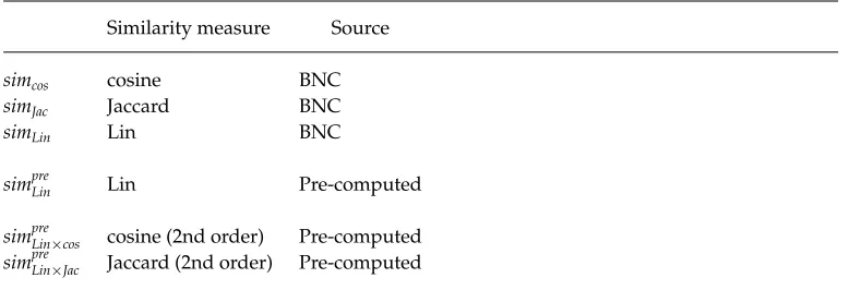
Table 7

Summary of distributional similarity measures used in this work.

Similarity measure Source

simcos cosine BNC

simJac Jaccard BNC

simLin Lin BNC

simpre_Lin Lin Pre-computed

simpre_Lin×cos cosine (2nd order) Pre-computed simpre_Lin×Jac Jaccard (2nd order) Pre-computed

2,000 basis elements. We tested Jaccard, cosine, and Lin’s measure for similarity, yielding

simJac,simcos, andsimLin, respectively.

In addition to measuring the similarity of two words directly, that is, using the co-occurrence vectors of each word as in Section 2, we also tried a variant which we will callsecond-order similarity. In this case each word is represented by a vector which contains all similar words with weights, where those weights come from first order similarity. That is, in order to obtain the second-order vector for wordw, we need to compute its first order similarity with all other words in the vocabulary. The second-order similarity of two words is then computed according to those vectors. For this, we just need to change the definition ofTandTin the similarity formulas in Figure 1: Now

T(w) would return the list of words which are taken to be similar tow, andT(w) would return the same list but as a vector with weights.

This approximation is computationally expensive, as we need to compute the square matrix of similarities for all word pairs in the vocabulary, which is highly time-consuming. Fortunately, the pre-computed similarity scores of Lin (1998) (which use

simLin) are readily available, and thus the second-order similarity vectors can be easily computed. We used Jaccard and cosine to compute the similarity of the vectors, and we will refer to these similarity measures assimpre_Lin×Jacandsimpre_Lin×coshereinafter. Due to the computational complexity, we did not compute second order similarity for the semantic space software of Pad ´o and Lapata (2007).

Table 7 summarizes all similarity measures used in this study, and the corpus or pre-computed similarity list used to build them.

3.4 Selectional Preferences for Prepositions

Table 8

Example ofprep-rolelexical models for the prepositionfrom, listed in alphabetical order.

Prep-role Number of Unique Examples

heads heads

from-Arg0 32 30 Abramson agency association barrier cut ...

from-Arg1 173 118 accident ad agency appraisal arbitrage ...

from-Arg2 708 457 academy account acquisition activity ad ...

from-Arg3 396 165 activity advertising agenda airport ...

from-Arg4 5 5 europe Golenbock system Vizcaya west

from-AM-ADV 19 17 action air air conception datum everyone ...

from-AM-CAU 5 4 air air design experience exposure

from-AM-DIR 79 71 agency alberta amendment america arson ...

from-AM-LOC 20 17 agency area asia body bureau orlando ...

from-AM-MNR 29 28 agency Carey company earnings floor ...

from-AM-TMP 33 21 april august beginning bell day dec. half ...

A particularly interesting case is that of prepositional phrases.8Prepositions define relations between the preposition attachment point and the preposition complement. Prepositions are ambiguous with respect to these relations, which allows us to talk about prepositionsenses. The Preposition Project (Litkowski and Hargraves 2005, 2006) is an effort that produced a detailed sense inventory for English prepositions, which was later used in a preposition sense disambiguation task at SemEval-2007 (Litkowski and Hargraves 2007). Sense labels are defined as semantic relations, similar to those of semantic role labels. In a more recent work, Srikumar and Roth (2011) presented a joint model for extended semantic role labeling in which they show that determining the sense of the preposition is mutually related to the task of labeling the argument role of the prepositional phrase. Following the previous work, we also think that prepositions define implicit selectional preferences, and thus decided to explore the use of preposi-tional preferences with the aim of improving the selection of the appropriate semantic roles. Addressing other arguments with non-nominal heads has been intentionally left for further work.

The most straightforward way of including prepositional information in SP models would be to add the preposition as an extra parameter of the SP. Initial experiments revealed sparseness problems with collecting the verb, preposition, NP-head, role 4-tuples from the training set. A simpler approach consists of completely disregarding the verb information while collecting the prepositional preferences. That is, the selec-tional preference for a prepositionpand roleris defined as the union of all nounsw

found as heads of noun phrases embedded in prepositional phrases headed bypand labeled with semantic roler. Then, one can apply any of the variants described in the previous sections to calculateSP(p,r,w). Table 8 shows a sample of the lexical model for the prepositionfrom, organized according to the roles it plays.

These simple prep-rolepreferences largely avoided the sparseness problem while still being able to capture relevant information to distinguish the appropriate roles in many PP arguments. In particular, they proved to be relevant to distinguish between adjuncts of the type “[in New York]Location” vs. “[in Winter]Temporal.” Nonetheless, we

are aware that not taking into account verb information also introduces some lim-itations. In particular, the simplification could damage the performance on PP core arguments, which are verb-dependent.9 For instance, our prepositional preferences would not be able to suggest appropriate roles for the following two PP arguments: “increase [from seven cents a share]Arg3” and “receive [fromthe funds]Arg2,” because

the two head nouns (cents and funds) are semantically very similar. Assigning the correct roles in these cases clearly depends on the information carried by the verbs.

Arg3is thestarting pointfor the predicateincrease, whereasArg2refers to thesourcefor

receive.

Our perspective on making this simple definition ofprep-roleSPs was practical and just a starting point to play with the argument preferences introduced by prepositions. A more complex model, distinguishing between prepositional phrases in adjunct and core argument positions, should be able to model the linguistics better yet alleviate the sparseness problem, and would hopefully produce better results.

The combination scheme for applying verb-roleand prep-roleis also very simple. Depending on the syntactic type of the argument we apply one or the other model, both in learning and testing:

r

preferences.

r

selectional preferences.

We thus use a straightforward method to combine both kinds of SPs. More complex possibilities like doing mixtures of both SPs are left for future work.

3.5 Role Classification with SP Models

Selectional preference models can be directly used to perform role classification. Given a target predicatepand noun phrase candidate argument with headw, we simply select the role r of the predicate which best fits the head according to the SP model. This selection rule is formalized as:

ROLE(p,w)=arg max

r∈Roles(p)SP(p,r,w) (11)

with Roles(p) being the set of all roles applicable to the predicate p, and SP(p,r,w) the goodness of fit of the selectional preference model for the head w, which can be instantiated with all the variants mentioned in the previous subsections, including the lexical model (Equation (8)) WordNet-based SP models (Equations (3) and (10)), and distributional SP models (Equation (7)), using different similarity models as in Table 7. Ties were broken returning the role coming first according to alphabetical order. Note that in the case ofSPwn (Equation 10) we need to use arg min rather than arg max.

Note that if the candidate argument is a prepositional phrase with preposition p

and embedded NP head wordw, the classification rule uses theprep-roleSP model, that is:

ROLE(p,p,w)=arg max r∈Roles(p)SP(p

_,r,w)

4. Experiments with Selectional Preferences in Isolation

In this section we evaluate the ability of selectional preference models to discriminate among different roles. For that, SP models will be used in isolation, according to the clas-sification rule in Equation (11), to predict role labels for a set of (predicate,argument-head) pairs. That is, we are interested in the discriminative power of the semantic information carried by the SPs, factoring out any other feature commonly used by the state-of-the-art SRL systems. The data sets used and the experimental results are presented in the following.

4.1 Data Sets

The data used in this work are the benchmark corpus provided by the CoNLL-2005 shared task on SRL (Carreras and M`arquez 2005). The data set, of over 1 million tokens, comprises PropBank Sections 02–21 for training, and Sections 24 and 23 for develop-ment and testing, respectively. The Selectional Preferences impledevelop-mented in this study are not able to deal with non-nominal argument heads, such us those of NEG, DIS, MOD (i.e., SPs never predict NEG, DIS, or MOD roles); but, in order to replicate the same evaluation conditions of typical PropBank-based SRL experiments all arguments are evaluated. That is, our SP models don’t return any prediction for those, and the evaluation penalizes them accordingly.

The predicate–role–head triples (p,r,w) for generalizing the selectional preferences are extracted from the arguments of the training set, yielding 71,240 triples, from which 5,587 different predicate-role selectional preferences (p,r) are derived by instantiating the different models in Section 3. Tables 9 and 10 show additional statistics about some of the most (and least) frequent verbs and prepositions in these tuples.

The test set contains 4,134 pairs (covering 505 different predicates) to be classified into the appropriate role label. In order to study the behavior on out-of-domain data, we also tested on the PropBanked part of the Brown corpus (Marcus et al. 1994). This corpus contains 2,932 (p,w) pairs covering 491 different predicates.

4.2 Results

The performance of each selectional preference model is evaluated by calculating the customary precision (P), recall (R), and F1 measures.10 For all experiments

re-ported in this paper, we checked for statistical significance using bootstrap resampling (100 samples) coupled with one-tailed paired t-test (Noreen 1989). We consider a result significantly better than another if it passes this test at the 99% confidence interval.

10P=Correct/Predicted∗100,R=Correct/Gold∗100, whereCorrectis the number of correct predictions, Predictedis the number of predictions, andGoldis the total number of gold annotations.

Table 9

Statistics of the three most and least frequent verbs in the training set. Role frame lists the types of arguments seen in training for each verb; Heads indicates the total number of arguments for the verb; Heads per role shows the average number of head words for each role; and Unique heads per role lists the average number of unique head words for each verb’s role.

Verb Role frame Heads Heads Unique heads

per role per role

say Arg0,Arg1,Arg3,AM-ADV, AM-LOC, 7,488 1,069 371

AM-MNR, AM-TMP, AM-LOC,AM-MNR

have Arg0,Arg1,AM-ADV,AM-LOC 3,487 498 189

AM-MNR,AM-NEG,AM-TMP

make Arg0,Arg1,Arg2,AM-ADV 2,207 315 143

AM-LOC,AM-MNR,AM-TMP

... ... ... ... ...

accrete Arg1 1 1 1

accede Arg0 1 1 1

absolve Arg0 1 1 1

Table 10

Statistics of the three most and least frequent prepositions in the training set. Role frame lists the types of arguments seen in training for each preposition; Heads indicates the total number of arguments for the preposition; Heads per role shows the average number of head words for each role; and Unique heads per role lists the average number of unique head words for each preposition’s role.

Preposition Role frame Heads Heads Unique heads

per role per role

in Arg0,Arg1,Arg2,Arg3,Arg4,Arg5 6,859 403 81

AM-ADV,AM-CAU,AM-DIR,AM-DIS, AM-EXT,AM-LOC,AM-MNR,AM-NEG, AM-PNC,AM-PRD,AM-TMP

to Arg0,Arg1,Arg2,Arg3,Arg4, 3,495 233 94

AM-ADV,AM-CAU,AM-DIR,AM-DIS, AM-EXT,AM-LOC,AM-MNR,AM-PNC, AM-PRD,AM-TMP

for Arg0,Arg1,Arg2,Arg3,Arg4, 2,935 225 74

AM-ADV,AM-CAU,AM-DIR,AM-DIS, AM-LOC,AM-MNR,AM-PNC,AM-TMP

... ... ... ... ...

beside Arg2, AM-LOC 2 1 1

atop Arg2, AM-DIR 2 1 1

aboard AM-LOC 1 1 1

Tables 11 and 12 list the results of the various selectional preference models in isolation. Table 11 shows the results for verb-role SPs, and Table 12 lists the results for the combination ofverb-roleandpreposition-roleSPs as described in Section 3.4.11

It is worth noting that the results of Tables 11 and 12 are calculated over exactly the

Table 11

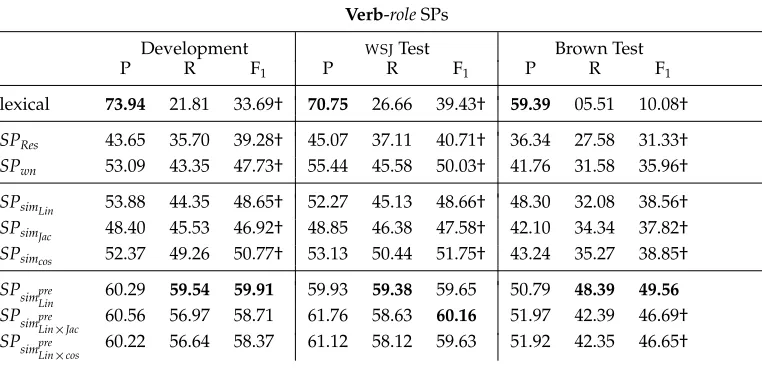
Results forverb-roleSPs in the development partition of WSJ, the test partition of WSJ, and the Brown corpus. For each experiment, we show precision (P), recall (R), and F1. Values in boldface font are the highest in the corresponding column. F1values marked with † are significantly lower than the highest F1score in the same column.

Verb-roleSPs

Development WSJTest Brown Test

P R F1 P R F1 P R F1

lexical 73.94 21.81 33.69† 70.75 26.66 39.43† 59.39 05.51 10.08†

SPRes 43.65 35.70 39.28† 45.07 37.11 40.71† 36.34 27.58 31.33† SPwn 53.09 43.35 47.73† 55.44 45.58 50.03† 41.76 31.58 35.96†

SPsimLin 53.88 44.35 48.65† 52.27 45.13 48.66† 48.30 32.08 38.56† SPsimJac 48.40 45.53 46.92† 48.85 46.38 47.58† 42.10 34.34 37.82† SPsimcos 52.37 49.26 50.77† 53.13 50.44 51.75† 43.24 35.27 38.85†

SP_simpre

Lin 60.29 59.54 59.91 59.93 59.38 59.65 50.79 48.39 49.56 SP_simpre

Lin×Jac 60.56 56.97 58.71 61.76 58.63 60.16 51.97 42.39 46.69† SP_simpre

Lin×cos 60.22 56.64 58.37 61.12 58.12 59.63 51.92 42.35 46.65†

Table 12

Results for combinedverb-roleandprep-roleSPs in the development partition of WSJ, the test partition of WSJ, and the Brown corpus. For each experiment, we show precision (P), recall (R), and F1. Values in boldface font are the highest in the corresponding column. F1values marked with † are significantly lower from the highest F1score in the same column.

Preposition-roleandVerb-roleSPs

Development WSJTest Brown Test

P R F1 P R F1 P R F1

lexical 82.05 39.17 53.02† 82.98 43.77 57.31† 68.47 13.60 22.69†

SPRes 63.72 53.09 57.93† 63.47 53.24 57.91† 55.12 44.15 49.03† SPwn 71.72 59.68 65.15† 65.70 63.88 64.78† 60.08 48.10 53.43†

SPsimLin 63.84 54.58 58.85† 63.75 56.40 59.85† 54.27 39.96 46.04† SPsimJac 61.75 61.13 61.44† 61.83 61.40 61.61† 55.42 53.45 54.42† SPsimcos 64.81 64.17 64.49† 64.67 64.22 64.44† 56.56 54.54 55.53†

SP_simpre

Lin 67.78 67.10 67.44† 68.34 67.87 68.10† 58.43 56.35 57.37† SP_simpre

Lin×Jac 69.90 69.20 69.55 70.82 70.33 70.57 62.37 60.15 61.24 SP_simpre

Lin×cos 69.47 68.78 69.12 70.28 69.80 70.04 62.36 60.14 61.23

penalized in recall. WordNet based models, which have a lower word coverage com-pared to distributional similarity–based models, are also penalized in recall.

In both tables, the lexical row corresponds to the baseline lexical match method. The following rows correspond to the WordNet-based selectional preference models. The distributional models follow, including the results obtained by the three similarity formulas on the co-occurrences extracted from the BNC (simJac,simcos simLin), and the results obtained when using Lin’s pre-computed similarities directly (simpre_Lin) and as a second-order vector (simpre_Lin×Jacandsimpre_Lin×cos).

First and foremost, this experiment proves that splitting SPs into verb- and

preposition-role SPs yields better results. The comparison of Tables 11 and 12 shows that the improvements are seen for both precision and recall, but especially remarkable for recall. The overall F1improvement is of up to 10 points. Unless stated otherwise, the

rest of the analysis will focus on Table 12.

As expected, the lexical baseline attains a very high precision in all data sets, which underscores the importance of the lexical head word features in argument classification. Its recall is quite low, however, especially in Brown, confirming and extending Pradhan, Ward, and Martin (2008), who also report a similar performance drop for argument classification on out-of-domain data. All our selectional preference models improve over the lexical matching baseline in recall, with up to 24 absolute percentage points in the WSJ test data set and 47 absolute percentage points in the Brown corpus. This comes at the cost of reduced precision, but the overall F-score shows that all selectional preference models are well above the baseline, with up to 13 absolute percentage points on the WSJ data sets and 39 absolute percentage points on the Brown data set. The results, thus, show that selectional preferences are indeed alleviating the lexical sparseness problem.12

As an example, consider the following head words of potential arguments of the verbwearfound in the test set:doctor,men,tie,shoe. None of these nouns occurred as heads of arguments of wear in the training data, and thus the lexical feature would be unable to predict any role for them. Using selectional preferences, we successfully assigned theA0role todoctorandmen, and theA1role totieandshoe.

Regarding the selectional preference variants, WordNet-based and first-order distri-butional similarity models attain similar levels of precision, but the former have lower recall and F1. The performance loss on recall can be explained by the limited lexical

coverage of WordNet when compared with automatically generated thesauri. Examples of words missing in WordNet include abbreviations (e.g.,Inc.,Corp.) and brand names (e.g.,Texaco,Sony).

The comparison of the WordNet-based models indicates that our proposal for a lighter method of WordNet-based selectional preference was successful, as our simpler variant performs better than Resnik’s method. In manual analysis, we realized that Resnik’s model tends to always predict the most frequent roles whereas our model covers a wider role selection. Resnik’s tendency to overgeneralize makes more frequent roles cover all the vocabulary, and the weighting system penalizes roles with fewer occurrences.

The results for distributional models indicate that the SPs using Lin’s ready-made thesaurus (simpre_Lin) outperforms Pad ´o and Lapata’s distributional similarity model (Pad ´o and Lapata 2007) calculated over the BNC (simLin) in both Tables 11 and 12. This might be due to the larger size of the corpus used by Lin, but also by the fact that Lin used a newspaper corpus, compared with the balanced BNC corpus. Further work would be needed to be more conclusive, and, if successful, could improve further the results of some SP models.

Among the three similarity metrics using Pad ´o and Lapata’s software, the cosine seems to perform consistently better. Regarding the comparison between first-order and order using pre-computed similarity models, the results indicate that second-order is best when using both theverb-roleandprep-rolemodels (cf. Table 12), although the results forverb-rolesare mixed (cf. Table 11). Jaccard seems to provide slightly better results than cosine for second-order vectors.

In summary, the use of separateverb-roleandprep-rolemodels produces the best results, and second-order similarity is highly competitive. As far as we know, this is the first time thatprep-rolemodels and second-order models are applied to selectional preference modeling.

5. Semantic Role Classification Experiments

In this section we advance the use of SP in SRL one step further and show that selec-tional preferences are able to effectively improve performance of a state-of-the-art SRL system. More concretely, we integrate the information of selectional preference models in a SRL system and show significant improvements in role classification, especially when applied to out-of-domain corpora.13

We will use some of the selectional preference models presented in the previous section. We will focus on the combination ofverb-roleandprep-rolemodels. Regarding the similarity models, we will choose the best two performing models from each of the three families that we tried, namely, the two WordNet models, the two best models based on the BNC corpus (simJac,simcos), and the two best models based on Lin’s precom-puted similarity metrics (sim2_Jac,sim2cos). We left the exploration of other combinations for future work.

5.1 Integrating Selectional Preferences in Role Classification

For these experiments, we modified theSwiRLSRL system, a state-of-the-art semantic role labeling system (Surdeanu et al. 2007).SwiRLranked second among the systems that did not implement model combination at the CoNLL-2005 shared task and fifth overall (Carreras and M`arquez 2005). Because the focus of this section is on role classi-fication, we modified the SRC component ofSwiRLto use gold argument boundaries, that is, we assume that semantic role identification works perfectly. Nevertheless, for a realistic evaluation, all the features in the role classification model are generated using actual syntactic trees generated by the Charniak parser (Charniak 2000).

The key idea behind our approach is model combination: We generate a battery of base models using all resources available and we combine their outputs using multi-ple strategies. Our pool of base models contains 13 different models: The first is the

unmodified SwiRL SRC, the next six are the selected SP models from the previous section, and the last six are variants ofSwiRLSRC. In each variant, the feature set of the unmodified SwiRLSRC model is extended with a single feature that models the choice of a given SP, for example, SRC+SPrescontains an extra feature that indicates the choice of Resnik’s SP model.14

We combine the outputs of these base models using two different strategies: (a) majority voting, which selects the label predicted by most models, and (b) meta-classification, which uses a supervised model to learn the strengths of each base model. For the meta-classification model, we opted for a binary classification approach: First, for each constituent we generatendata points, one for each distinct role label proposed by the pool of base models; then we use a binary meta-classifier to label each candidate role as either correct or incorrect. We trained the meta-classifier on the usual PropBank training partition, using 10-fold cross-validation to generate outputs for the base models that require the same training material. At prediction time, for each candidate constituent we selected the role label that was classified as correct with the highest confidence.

The binary meta-classifier uses the following set of features:

r

indicates that the SRC+SPresbase model proposed the Arg0 label. We add 13 such features, one for each base model. Intuitively, this feature allows the meta-classifier to learn the strengths of each base model with respect to role labels: SRC+SPresshould be trusted for the Arg0 role, and so on.

r

featureMajority=trueindicates that the majority of the base models proposed the same label as the one currently considered by the meta-classifier.

r

for each number of base models,N, we generateNdistinct features indicating that the number of base models that proposed this label is larger thank, wherek∈[0,N). For example, if two base models proposed the label under consideration, we generate the following two features: BaseModelNumber>0andBaseModelNumber>1. This feature provides finer control over the number of votes received by a label than the majority voter, for example, the meta-classifier can learn to trust a label if more than two base models proposed it, even if the majority vote disagrees.

r

distinct feature for each base model that proposed the current label, and also a concatenation of all these base model names. The latter feature is designed to allow the meta-classifier to learn preferences for certain combinations of base models. For example, if two base models,SPresand

SPwn, proposed the label under consideration, we generate three features: Base=SPres,Base=SPwn, andBase=SPres+SPwn.

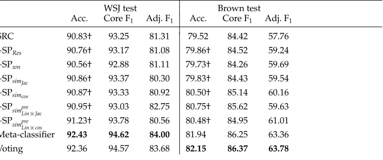
Table 13

Results for the combination approaches. Accuracy shows the overall results. Core and Adj contain F1results restricted to the core numbered roles and adjuncts, respectively. SRC is SwiRL’s standalone SRC model; +SPxstands for the SRC model extended with a feature given by

the corresponding SP model. Values in boldface font are the highest in the corresponding column. Accuracy values marked with † are significantly lower than the highest accuracy score in the same column.

WSJ test Brown test

Acc. Core F1 Adj. F1 Acc. Core F1 Adj. F1

SRC 90.83† 93.25 81.31 79.52 84.42 57.76

+SPRes 90.76† 93.17 81.08 79.86† 84.52 59.24

+SPwn 90.56† 92.88 81.11 79.73† 84.26 59.69

+SPsimJac 90.86† 93.37 80.30 79.83† 84.43 59.54 +SPsimcos 90.87† 93.33 80.92 80.50† 85.14 60.16 +SP_simpre

Lin×Jac 90.95† 93.03 82.75 80.75† 85.62 59.63 +SP_simpre

Lin×cos 91.23† 93.78 80.56 80.48† 84.95 61.01 Meta-classifier 92.43 94.62 84.00 81.94 86.25 63.36

Voting 92.36 94.57 83.68 82.15 86.37 63.78

5.2 Results for Semantic Role Classification

Table 13 compares the performance of both combination approaches against the stand-alone SRC model. In the table, the SRC+SP∗models stand for SRC classifiers enhanced with one feature from the corresponding SP. The meta-classifier shown in the table com-bines the output of all the 13 base models introduced previously. We implemented the meta-classifier using Support Vector Machines (SVMs)15 with a quadratic polynomial kernel, andC=0.01 (tuned in the development set).16Lastly, Table 13 shows the results of the voting strategy, over the same set of base models.

In the columns we show overall classification accuracy and F1results for both core

arguments (Core) and adjunct arguments (Adj.). Note that for the overall SRC scores, we report classification accuracy, defined as ratio of correct predictions over total number of arguments to be classified. The reason for this is that the models in this section always return a label for all arguments to be classified, and thus accuracy, precision, recall, and F1are all equal.

Table 13 indicates that four out of the six SRC+SP∗models perform better than the standalone SRC model in domain (WSJ), and all of them outperform SRC out of domain (Brown). The improvements are small, however, and, generally, not statistically signifi-cant. On the other hand, the meta-classifier outperforms the original SRC model both in domain (17.4% relative error reduction; 1.60 points of accuracy improvement) and out of domain (13.4% relative error reduction; 2.42 points of accuracy improvement), and the differences are statistically significant. This experiment proves our claim that SPs can be successfully used to improve semantic role classification. It also underscores the fact that combining SRC and SPs is not trivial, however. Our hypothesis is that this

15http://svmlight.joachims.org.